Abstract

By using scattering in near field techniques, a microscope can be easily turned into a device measuring static and dynamic light scattering, very useful for the characterization of nanoparticle dispersions. Up to now, microscopy based techniques have been limited to forward scattering, up to a maximum of $30^{\circ}$. In this paper we present a novel optical scheme that overcomes this limitation, extending the detection range to angles larger than $90^{\circ}$ (back-scattering). Our optical scheme is based on a microscope, a wide numerical aperture objective, and a laser illumination, with the collimated beam positioned at a large angle with respect to the optical axis of the objective (Tilted Laser Microscopy, TLM). We present here an extension of the theory of near field scattering, which usually applies only to paraxial scattering, to our strongly out-of-axis situation. We tested our instrument and our calculations with calibrated spherical nanoparticles of several different diameters, performing static and dynamic scattering measurements up to $110^{\circ}$. The measured static spectra and decay times are compatible with the Mie theory and the diffusion coefficients provided by the Stokes-Einstein equation. The ability of performing backscattering measurements with this modified microscope opens the way to new applications of scattering in near field techniques to the measurement of systems with strongly angle dependent scattering.

Nanoparticle characterization by using Tilted Laser Microscopy:

back scattering measurement in near field.

D. Brogioli, D. Salerno, V. Cassina, and F. Mantegazza

Dipartimento di Medicina Sperimentale, Università degli Studi di Milano - Bicocca, Via Cadore 48, Monza (MI) 20052, Italy.

OCIS codes: (120.5820) Scattering measurements; (290.5820) Scattering measurements; (290.5850) Scattering, particles; (100.2960) Image analysis.

1 Introduction.

Optical microscopy and light scattering are widely used, well-known techniques, often applied to the study of samples such as biomedical systems, colloidal suspensions, or complex fluids. Traditionally, the instruments for implementing optical microscopy and light scattering belong to two well distinct groups. Optical microscopes are imaging tools, that is, they provide a deterministic mapping of an object’s optical properties, collecting light in the so-called near field. Conversely light scattering devices measure statistical properties, detecting the light scattered in the far field [6, 7, 8, 9, 10]. Accordingly, traditional light scattering methods can be conveniently renamed as Scattering In the Far Field (SIFF) techniques.

A whole family of alternative methods have been developed for measuring the scattered light intensity fluctuations in the near field, similarly to what is done in microscopy. Several different names have been introduced to describe these specific slightly different methods, often independently developed by different communities. Here we will call this family: Scattering In the Near Field (SINF) [11, 12], as opposed to SIFF. The community interested in laser speckles developed the Near Field Speckle (or Scattering) (NFS) techniques, first in the homodyne version [13, 14] and then in heterodyne version, Heterodyne Near Field Speckles (HNFS) [15, 16, 17]. Similar techniques, but applied to imaging configurations are shadowgraph [18, 19] and schlieren [20]. In turn, these bear a strong similarity with Gabor’s in-line holography [21]. Furthermore, the community devoted to holography have also used a similar approach for back scattering detection [22]. Finally, microscopists reported Fourier Transform Light Scattering [23] and Differential Dynamic Microscopy [24]. However, an exaustive list of SINF techniques is out of the scope of a paper.

Some years ago, the interest in the development of a hybrid instrument, combining optical microscopy and light scattering, led to the development of optical systems able to record simultaneously the near and the far field light intensities [25, 26, 27, 28]. Unfortunately the extreme complexity of the experimental set-ups limited the spread of these techniques.

SINF techniques proved to be a very simple and efficient way to use a microscope in order to measure static light scattering [13, 14, 20] or dynamic light scattering of nanoparticles [29], depolarized dynamic light scattering of rod-like nanoparticles [11] and biological samples [23]. Generally the dynamics is extracted by means of a so-called “differential” algorithm presented in References [30, 31, 32, 33], which has also been used with white light [24] and X-rays illumination [34]; moreover it has been used for exctracting static data [17]. Since the algorithm involves fast grabbing of the images, a further simplifying step is constituted by the “exposure time dependent spectrum” (ETDS) procedure [11, 35], which drops the requirement of a fast acquisition.

All the above SINF experiments have been limited to small scattering angles, up to about $30^{\circ}$, the main limitation being the numerical aperture of the collecting objective. By using larger numerical aperture, the maximum detectable scattering angle can be increased, but, the $90^{\circ}$ limit remains inaccessible.

In this paper, we describe a novel detection scheme able to overcome this limitation and allowing detecting the scattered light up to the back scattering regime, (more than $90^{\circ}$). Experimental data will be presented for scattering angles up to $110^{\circ}$, almost four times larger than what ever reported in a previous SINF measurement. Potentially the method can be extended to even larger scattering angles, approaching $180^{\circ}$.

The basic idea of the method is to illuminate the sample with a tilted beam of coherent light, whence the name of Tilted Laser Microscopy (TLM). Indeed, whereas in a conventional SINF experiment a laser beam is sent through the sample along the axis of the collecting optics, in the described apparatus the laser beam enters into the system at a large angle with respect to the optical axis. In the proposed optical scheme, the aperture of the objective and the tilt angle are chosen so that the transmitted and the scattered beams are both collected by the objective. This approach is different from the classical “dark field” microscopy: in dark field the transmitted beam is deliberately removed, while in TLM the unscattered and scattered beams overlap.

The importance of collecting the scattering at large angles lies in the fact that the scattered light can contain details which are very important for nanoparticle characterization. For example, very small particles scatter light almost isotropically, while larger ones (sometimes contaminants or impurities) scatter more strongly in the forward direction, and so often disturb the detection of the nanoparticle signal at low scattering angles. Thus the possibility of distinguishing nanoparticles is directly related to the ability of getting information about the light scattered in the backward direction. The proposed technique is an answer to this problem of the low signal in nanoparticle scattering measurements. On the other hand, the scattering signal frequently shows interesting features at large angles not accessible with traditional SINF methods. Several scientific milestones of soft matter (fractal dimension of colloidal aggregates, gel/glass properties, liquid crystals structures, etc.) has been demonstrated by studying the structure factor of the system, up to high wave vectors.

2 Scattering In the Near Field tutorial.

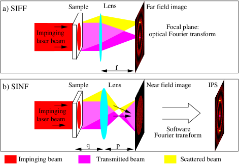
Fig. 1: Schematic description of scattering detection techniques. The red, yellow, and magenta beams represent the impinging, scattered and transmitted beams respectively. Panel a: traditional Scattering In Far Field (SIFF) technique. The scheme refers to a typical small angle light scattering; other SIFF techniques are based on the same principle. The beam scattered at a given angle is focused by the lens into one point (yellow dot) on the observation plane, where the far field image is collected. Panel b: Scattering In Near Field (SINF) technique. The reported scheme refers to shadowgraph technique, and is quite similar to HNFS configuration; other SINF techniques are based on the same principle, with slightly different schemes. A near field image of a plane close to the sample is formed on the observation plane. The scattered and the transmitted beams are both interfering on the observation plane. The near field Image Power Spectrum (IPS) is then evaluated through a Fourier transform. The yellow beam generates two points (yellow dots) on the IPS

In this section the general ideas of Light Scattering are briefly and quantitatively reviewed, comparing the SINF outputs with the results of the classical SIFF technique. First, an informal and intuitive discussion about the physics of Light Scattering is provided, including a description of the traditional far field techniques. Second, we discuss some peculiarities of the near field method, focusing on the heterodyne scheme. A more detailed and systematic description of SIFF can be found in classical references [6, 7, 8, 9, 10], whereas rigorous presentations of SINF can be found in [15, 13, 14, 19, 20, 17, 36].

Generally speaking, a sample scatters light if its fluctuations of concentration and temperature induce refractive index fluctuations. In a standard light scattering experiment the intensity of the scattered light $I\left(\vartheta,\varphi\right)$ is measured at a given scattering angle $\vartheta$ and azimuthal angle $\varphi$. Then, for example, the scattering intensity from spherical colloids $I\left(\vartheta,\varphi\right)$ can be compared with the outcome of the exact Mie algorithm for determining the particle size.

A traditional SIFF experiment basically consists in measuring the scattered intensity at a given scattering angle selected by placing the detector along a given direction very far from the sample. The far field requirement is alternatively satisfied by placing a lens just beyond the sample and collecting the light at the lens focal plane (see Fig. 1-a). The intensity distribution thus obtained at the sensor plane exactly represents the far field image: the light scattered at a given angle falls on a given point $\left(\vartheta,\varphi\right)$ of the image. The effect of the lens is essentially that of performing the optical Fourier transform of the signal. The image (intensity mapping) is speckled, but with a well defined average intensity distribution, representing the time averaged scattering intensity. The speckled appearance is due to the stochastic interference between the beams scattered in the same direction by the different scatterers. Furthermore the 2D statistical intensity distribution of the speckles is an exponentially decaying function [37]. If the sample is not static in time, the intensity of the speckle field is fluctuating (boiling) on a time scale depending on the scattering angle $\vartheta$. For example, for a colloidal solution, the boiling is slow close to the forward direction $\vartheta=0$, while it seems faster at larger angles.

In a SINF measurement, a near field image is collected either directly by a pixilated sensor placed in front of the sample, or via an optical imaging system (see Fig. 1-b). The scheme reported in Fig. 1-b refers to shadowgraph technique, and is quite similar to HNFS configuration; other SINF techniques are based on the same principle, with slightly different schemes. The near field image consists in the patterns generated by interference between the overlapping scattered beam and much more intense transmitted beam (heterodyne detection). Each scattered beam generates a Fourier mode on the near field image; thus the image decomposition into Fourier modes allows the determination of the scattered beam intensities. Indeed the near field Image Power Spectrum (IPS) is then calculated in silico by means of a 2D Fast Fourier Transform software. The obtained IPS is very similar to the far field image obtained in the SIFF experiment: essentially the same information is obtained by means of a software elaboration on the SINF image, instead of the optical Fourier transform given by the SIFF image.

However, some important differences between the IPS and the far field image can be noticed.

1. A single scattered beam gives rise to two points on the IPS. For example the yellow beam of 1-b generates the two points marked with the yellow dots on the IPS. In other words, the single yellow dot shown in the far field image of Fig. 1-a corresponds to two yellow dots in the IPS of Fig. 1-b. This effect is related to a fundamental property of the Fourier transform, which is not able to distinguish between the two symmetric beams generating a given mode within the image.

2. The 2D statistical intensity distribution of the speckles in a SINF image has, with very good approximation, a Gaussian distribution [37], resulting from heterodyne superposition of the scattered and transmitted beams. As already stated, the SIFF speckles show a 2D exponentially decaying statistics [37].

3. Also the dynamics is different: SINF and SIFF images are intrinsically related to the CCD exposure time in different ways. While different acquisition times in SINF correspond to a blurring of the fluctuations [11], in SIFF they correspond to different averages of speckle intensities. More explicitly, while in SINF a long exposure time reduces the power spectrum, in the SIFF case a long exposure time produces a less speckled appearance of the far field image.

4. The most simple SINF schemes are heterodyne, so that they measure one of the complex components of the radiation field, while homodyne SIFF measures only the intensity. As consequence, a near field image carries information about the phases. As a result, it is easy to perform velocimetry with the SINF heterodyne signal [38]. On the other hand, this sensitivity to phases can be seen as a drawback, since a diffusion measurement is vulnerable to collective motions.

5. While the SIFF signal provides a direct measurements of the scattered intensity, the SINF signal (the Image Power spectrum) is related to the scattering intensity via the transfer function of the system. The latter one, depending on geometry and scattering angles, may introduce not negligible corrections.

3 Tilted laser methods.

Figure 2 schematically describes how the here proposed TLM setup works. Basically, the scheme is analogous to the SINF design shown in Fig. 1-b, with the difference that in the tilted scheme the transmitted beam enters into the objective at a given angle $\alpha$. Thanks to the objective lens, a plane close to the sample is imaged on the 2D sensor, and this ensures that both the scattered and transmitted beams are overlapping and collected on the sensor.

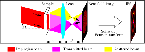
Fig. 2: Schematic description of Tilted Laser Microscopy technique. The red, yellow, and magenta beams represent the impinging, scattered and transmitted beams respectively. The impinging beam falls on the sample at angle $\alpha$ with respect to the optical axis of the system. A near field image of a plane close to the sample is formed on the observation plane. The near field Image Power Spectrum (IPS) is then evaluated through a Fourier transform. The yellow beam generates two points (yellow dots) on the IPS.

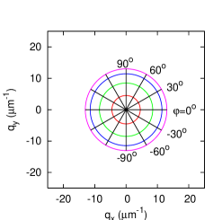
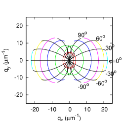
Fig. 3: Upper panels: schematic view of the geometry of the wave vectors corresponding to the incoming light ($\vec{K}_{i}$), the scattered light ($\vec{K}_{s}$), the transferred wave vector ($\vec{Q}$), and the 2D image wave vector ($\vec{q}$). $2\Theta$ is the maximum acceptance angle of the objective and $\alpha$ is the tilted angle. Lower panels: mapping of the IPS wave vector $\vec{q}$ as a function of scattering angle $\vartheta$ and azimuthal angle $\varphi$. Acceptance angle $\Theta=80^{\circ}$. Left panels: collinear illumination. Right panels: out-of-axis illumination.

We now discuss how to relate the value of the image wave vector $\vec{q}$ with the transferred wave vector $\vec{Q}$, which have to be taken into account when performing a TLM measurement. Fig. 3, upper panels, shows a schematic drawing of the geometrical arrangement of the wave vectors, for the two cases of collinear (left panels) and out-of-axis (right panels) illumination with tilt angle $\alpha$. The picture helps understand the physical mechanism by which TLM increases the range of collected scattering angles.

Consider an objective with a given numerical aperture, i.e. able to collect beams within an angle $\Theta$ with respect to its optical axis. If the illuminating beam is sent along the optical axis, then the maximum detectable scattering angle $\vartheta$ is at most $\Theta$.

TLM allows to nearly double this range. Indeed, with this geometry, the objective gathers the illuminated beam at an angle close to $\Theta$, together with the light scattered at the opposite side of the objective (see Fig. 3, upper row, right panel). In this case the angle between the transmitted beam and the scattered one can be close to $2\Theta$, taking advantage of the objective’s total numerical aperture.

A SINF measurement consists in collecting several images and then calculating their IPS $S\left(\vartheta,\varphi\right)$, that is the near field Image Power Spectrum, obtained, through a FFT algorithm, as the mean square of the Fourier transform of the images [15].

Each point in the IPS $S\left(\vec{q}\right)$ represents the amplitude of the Fourier mode with wave vector $\vec{q}$ of the near field images; or equivalently, it represents the light intensity $I\left(\vartheta,\varphi\right)$ at a given scattering angle $\vartheta$ and azimuthal angle $\varphi$.

In the following, we will describe the relationship between $\vec{q}$ and $\left(\vartheta,\varphi\right)$, which is essential to relate the obtained IPS $S\left(\vec{q}\right)$ to the scattered intensity $I\left(\vartheta,\varphi\right)$:

$$S\left[\vec{q}\left(\vartheta,\varphi\right)\right]=T\left(\vartheta,\varphi\right)I\left(\vartheta,\varphi\right)$$ (1)

where $T\left(\vartheta,\varphi\right)$ is the tranfer function of the optical system.

Fig. 3 shows the geometrical arrangement for the scattering wave vector $\vec{K}_{s}$, the impinging beam wave vector $\vec{K}_{i}$, the transferred wave vector $\vec{Q}=\vec{K}_{s}-\vec{K}_{i}$ and the 2D image wave vector $\vec{q}$. The image wave vector $\vec{q}$ is actually the 2D projection of the transferred wave vector $\vec{Q}$ on the plane perpendicular to the optical axis, i.e. the sensor plane. Therefore the $x$ and $y$ components of the two vectors $\vec{Q}$ and $\vec{q}$ are the same.

If the transferred wave vector $\vec{Q}$ is known, then the wave vector $\vec{q}$ on the image can be directly obtained:

$$\vec{q}\left(\vec{Q}\right)=\left(Q_{x},Q_{y},0\right)$$ (2)

Using this equation, $\vec{q}$ can also be expressed in terms of the scattering angle $\vartheta$, azimuthal angle $\varphi$ and the tilt angle $\alpha$ as:

$$\vec{q}\left(\vartheta,\varphi\right)=K\left[\cos\left(\alpha\right)\sin\left(\vartheta\right)\cos\left(\varphi\right)+\sin\left(\alpha\right)\cos\left(\vartheta\right)-\sin\left(\alpha\right),\sin\left(\vartheta\right)\sin\left(\varphi\right),0\right]$$ (3)

The inverse problem is somewhat tricker. If the image wave vector $\vec{q}$ is given, that is the actual experimental situation, then a third equation is necessary to get the third $z$ component of the transferred wave vector $\vec{Q}$. This can be obtained from the condition $\left|\vec{Q}+\vec{K}_{i}\right|=\left|\vec{K}_{s}\right|=K$, plus the condition $\vec{K}_{s}\cdot\hat{z}>0$ which allows choosing one of the two solutions of the quadratic equation. The relationship between the image and the transferred vector is therefore:

$$\vec{Q}\left(\vec{q}\right)=\left(q_{x},q_{y},\sqrt{\left(\vec{K}_{i}\cdot\hat{z}\right)^{2}-\vec{q}^{2}-2\vec{q}\cdot\vec{K}_{i}}-\vec{K}_{i}\cdot\hat{z}\right)$$ (4)

The graphs of $\vec{q}$ for values of scattering angle $\vartheta$ from $20^{\circ}$ up to $120^{\circ}$ and azimuthal angle $\varphi$ in steps of $30^{\circ}$ are shown in Fig. 3, lower panels, for collinear and tilted illumination. They represent the mapping of $\vartheta,\varphi$ on IPS images. It’s worth noting that each scattered beam at $\vartheta,\varphi$ corresponds to two points, $\vec{q}$ and $-\vec{q}$, in the IPS. The mapping $-\vec{q}\left(\vartheta,\varphi\right)$ is also shown in Fig. 3, represented by thin lines. It is evident that the out-of-axis illumination allows mapping of angles larger than $90^{\circ}$ in the IPS.

It’s worth noting that very large scattering angles $\vartheta$ are accessible only for azimuthal angles $\varphi$ nearly aligned with the illumination tilt plane, that is $\varphi\approx 0^{\circ}$. In the following, the mapping $\vec{q}\left(\vartheta,\varphi\right)$ will be used mainly to get the value of $I\left(\vartheta\right)$, that is, the average value of $I\left(\vartheta\right)$ over a small range of $\varphi$ around 0. If the polarization of the main beam is $\varphi=0^{\circ}$, the measured scattering component will be called “parallel”. In the opposite case, that is $\varphi=90^{\circ}$, we measure the “perpendicular” component.

4 Data processing.

By using Eq. 4 it is possible to relate the output of the Fourier analysis of the grabbed images $S\left(q\right)$ to the scattering intensity $I\left(Q\right)$. In order to evaluate the sample dynamics, further analysis can be implemented by using the so called Exposure-Time-Dependent Spectrum (ETDS) processing, which we recently reported in [11]. Essentially, the IPS is evaluated by taking images at various exposure times, thus actually obtaining the Exposure-Time-Dependent Spectrum $S\left(q,\Delta t\right)$ [35]. As $\Delta t$ is increased, the fluctuations average out, leading to a decrease in the ETDS signal. For example, for Brownian colloidal particles, the ETDS decreases strongly at large scattering angles $\vartheta$. For very long $\Delta t$, all the fluctuations are washed out, and the resulting images contain only the optical background plus the fluctuating instrumental noise $B\left(q\right)$. In this way, the ETDS gives access to a quantitative measurement of the system dynamics. Indeed, it is possible to analytically derive a theoretical expression for the $S\left(q,\Delta t\right)$, and thus to get the diffusion coefficient of the particles by using a fitting procedure [35, 11]. When a negligible $\Delta t$ is considered, the “instantaneous” IPS $S\left(q\right)$ is obtained, as described by Eq. 1. When $\Delta t$ is not negligible with respect to the sample dynamics, the ETDS is accordingly modified [11]. For colloidal samples, the time correlation function is a decreasing exponential with decay time $\tau=1/(DQ^{2})$, where $D$ is the translational diffusion coefficient of the nanoparticles. In this case the ETDS is expressed as [11, 35]:

$$S\left[q\left(\vartheta,\varphi\right),\Delta t\right]=T\left(\vartheta,\varphi\right)I\left(\vartheta,\varphi\right)f\left(\frac{\Delta t}{\tau}\right)$$ (5)

where:

$$f\left(x\right)=2\frac{e^{-x}-1+x}{x^{2}}$$ (6)

The procedure for obtaining the decay time $\tau$ consists in acquiring a series of images with many different exposure times, in analyzing the ETDS $S\left[q\left(\vartheta,\varphi\right),\Delta t\right]$ for each scattering angle as a function of the exposure time, and finally in fitting it with Eq. 5, keeping $\tau$ as free parameter. By using this procedure, a direct measurement of the time constants for all the measured wave vectors is simultaneously achieved. Moreover, the static scattered intensity $I\left(\vartheta,\varphi\right)$, multiplied by the transfer function $T\left(\vartheta,\varphi\right)$ is obtained, in analogy with the procedure developed for the calculation of the structure function in [32, 33]. In general, the instrument transfer function $T\left(\vartheta,\varphi\right)$ can significantly depend on the wave vector, such as in the shadowgraph [39]. On the contrary, in the near field scattering regime, the transfer function is slowly varying within the accessible scattering range [17]. The transfer function was actually evaluated by performing calibration measurements on known samples, so that a direct access to the static scattered intensity of our sample can be obtained.

5 Experimental set up.

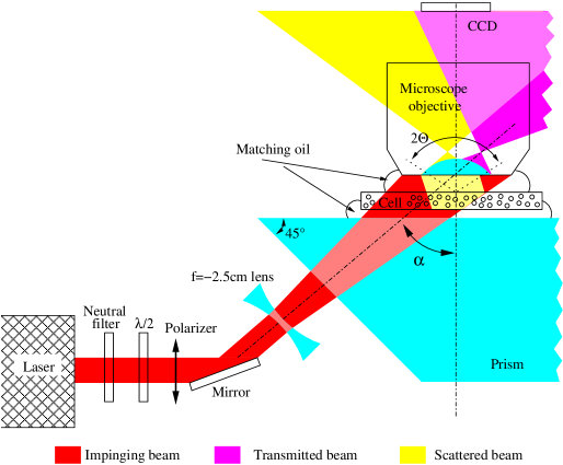
Fig. 4: Sketch of the optical set-up. The He-Ne laser generates a collimated laser beam, which is attenuated by a neutral filter. A half-wave plate and a polarizer control the beam polarization. A mirror bends and adjusts the beam direction. The beam is then expanded by means of a negative focal-length lens, making it slightly divergent. The beam goes through a $45^{\circ}$ prism, and enters the sample cell with about a $\alpha=45^{\circ}$ angle with respect to the vertical. Scattered light is acquired in the near field, together with transmitted light, through a vertical microscope objective, which conjugates a plane close to the sample onto the CCD sensor.

In Fig. 4 a sketch of the optical set-up is shown. The experimental apparatus consists of a standard microscope equipped with a low-speed CCD camera (Andor Luca). The microscope core is made by a commercial infinite conjugate oil immersion objective (Nikon plan achromat) 100X, numerical aperture NA=1.25 and working distance 0.17 mm, used with a tube lens with half the nominal focal, so that the resulting magnification is 50X. Its acceptance angle is $\Theta=70^{\circ}$. Some figures in the present article report images and data obtained with a plan-achromatic 40X objective (Optika Microscopes, FLUOR), with 0.65 numerical aperture, to emphasize the effects of the finite acceptance angle $\Theta=30^{\circ}$.

The illuminating source of the microscope has been replaced by a $10\mathrm{mW}$ He-Ne laser (Nec), enlarged by a negative $-2.5\mathrm{cm}$ focal-length lens, making the beam diverge, and thus increasing its diameter up to about $4\mathrm{mm}$ at the sample plane. This use of a single lens instead of a beam expander introduces a small error of about $1^{\circ}$, which is negligible with respect to the large scattering angles we are interested in. The beam coming from the laser source is attenuated by a variable neutral-filter wheel, with transmission range $0.3-0.0003$, and is bent by a mirror at a fixed angle respect to the vertical axis. The polarization state of the impinging beam is controlled by a half-wavelength plate and a polarizer, placed perpendicularly to the beam and suitably oriented. After $20\mathrm{cm}$ the diverging beam enters a $45^{\circ}$ prism, in contact with the cell. The beam direction inside the cell is $\alpha=45^{\circ}$ with respect to the vertical. Without the aid of such a prism the maximum tilting angle is bound by the total reflection at the glass/air interface.

The scattered light is collected beyond the sample, together with the transmitted beam (heterodyne detection) in the near field by means of the microscope objective and the tube lens conjugating a plane close to the sample onto the CCD sensor plane.

The sample is placed in a glass cell of $1\mathrm{mm}$ optical path, made by two microscope cover slips, spaced by small glass strips cut from microscope slides, and glued with silicone rubber. Both couplings (prism/cell and cell/objective) are index matched by a standard microscope oil, with refractive index 1.55. The first focal plane of the objective is placed inside the sample, the exact position being not an important issue. The large beam size ensures that the imaged area receives light from a portion of illuminated sample, for any angle inside the range accepted by the objective, thus also satisfying the near field condition [29].

6 Materials

We studied different samples of commercial polystyrene calibrated spherical nano-particles. The different samples are listed in Tab. 1.

Sample	Producer	Nominal diameter (nm)	Dynamic SIFF measured diameter (nm)
A	Polyscience Inc.	20	23
B	Duke Scientific Corp.	80	81
C	Duke Scientific Corp.	150	149
D	Polyscience Inc.	400	402
E	Polyscience Inc.	1520	1620

Table 1: List of the analyzed samples.

The particles are dispersed in deionized water, and are used without further purification, neither dialysis nor salt adding. The particles are strictly mono-dispersed and their nominal sizes have been checked by a traditional dynamic SIFF apparatus, providing measured sizes shown in fourth column Tab. 1. Samples B and C, from Duke Scientific Corporation, are dynamic light scattering calibration standards; the measured diameters are in excellent agreement with nominal values, and the error is compatible with the variability between different samples, as reported by the producer. The same excellent agreement is found also for sample D from Polyscience. For what concerns samples A and E the error is larger, of the order of 10%, probably due to the aging. From now on, we will compare the data obtained with the TLM apparatus with the above data actually measured with dynamic SIFF, and not with the nominal values.

7 Results and discussion.

$\alpha=0^{\circ}$	$\alpha=12^{\circ}$	$\alpha=24^{\circ}$	$\alpha=45^{\circ}$

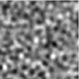
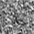
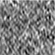
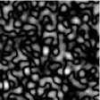
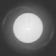
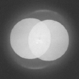
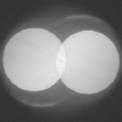
Fig. 5: Upper panels: 2D images of the SINF speckle field, taken at different tilt angles $\alpha$. The size of the images is $12.5\mathrm{\mu m}$ in real space. After software magnification, finite-pixel-size effects have been removed by suitable image processing for an easier visualization. The contrast of the image with $\alpha=45^{\circ}$ has been enhanced. Lower panels: power spectra of the same images, presented using a logarithmic intensity scale. The size of the image represents a wave vector $q=12\mathrm{\mu m}^{-1}$. The microscope objective is a 40X, 0.65 NA. The bright disks represent the heterodyne signal, given by the interference between the most intense transmitted beam and the scattered beam. The geometrical position of the disks depends on the tilt angle $\alpha$. A faint circular halo, centered in the IPS, represents the negligible homodyne signal, due to self interference between different scattered beams. The disks are surrounded by very faint whiskers due to spurious reflections. In the last column on the right, the image shows the homodyne contribution only, since the transmitted beam is stopped by the objective diaphragm, by deliberately using a tilting angle higher than the objective maximum acceptance angle. This last configuration cannot be used in TLM setup. Data obtained with sample C.

In Fig. 5, upper panels, typical near field images at different tilt angles $\alpha$ are shown as collected by a CCD, while in the lower panels the corresponding power spectra (IPS) are presented. We used for these images the sample C, which provides a sufficiently intense scattering almost on every scattering angle $\vartheta$. The employed objective is 40X, with an acceptance angle $\Theta=30^{\circ}$.

For collinear illumination ($\alpha=0$), the IPS shows a bright, nearly uniform circle at the center, corresponding to the nearly isotropically scattered light, clipped by the angular acceptance of the objective. The beams scattered at small angle $\vartheta$ are represented by the points close to the center of the IPS image. In general, the optical collecting system determines the scattering angle range which can be measured. In SIFF, this angular limitation produces a vignetting visible in the far field image. By comparison, as shown in Fig. 5, in SINF set up the acceptance angle of the microscope generates a vignetting in the near field IPS (Fourier space). On the other hand, the intensity distribution in the near field image (real space) shows a speckle pattern, superimposed on an average uniform intensity distribution with no intensity fading in the periphery of the image.

For out-of-axis illumination, the center of the IPS still represents beams with small scattering angle $\vartheta$, but, as the tilt angle $\alpha$ is increased, the vignetting circle is translated with respect to the center of the IPS, as previously shown in Fig. 3. This allows collecting light at larger scattering angles. It’s worth pointing out that the IPS is always center-symmetric, so that two clipping circles are visible in case of out-of-axis illumination. In this situation the centers of the shifted circles represent the beam scattered along the optical axis of the objective.

In Fig. 5, for every in-axis and out-of-axis images, a faded circular halo outside the brighter internal circles is also visible, due to the self interference (homodyne term) of the scattered light collected by the objective. Obviously, in our heterodyne detection scheme, the homodyne signal is not the object of our study and its intensity is negligible in the shown cases. The radius of the homodyne signal disk is twice the radius of the heterodyne disk. As apparent from Fig. 5, the size and position of the homodyne scattering circle is unaffected by the tilt angle $\alpha$.

In the following, we quantitatively explain the observed characteristics of the homodyne and heterodyne disks. The objective collects beams inside its aperture cone, that is, beams whose wave vector $\vec{K}_{s}=\left(K_{x},K_{y},K_{z}\right)$ satisfies the condition:

$$\sqrt{K_{x}^{2}+K_{y}^{2}}<K\sin\Theta.$$ (7)

When considering a transmitted beam with wave vector $\vec{K}_{i}=K\left(\sin\alpha,0,\cos\alpha\right)$, the transferred wave vector $\vec{Q}=\vec{K}_{s}-\vec{K}_{i}$ satisfies:

$$\sqrt{\left(Q_{x}+K\sin\alpha\right)^{2}+Q_{y}^{2}}<K\sin\Theta,$$ (8)

which describes the heterodyne signal disk, centered in $\vec{q}=\left(K\sin\alpha,0\right)$ with radius $K\sin\Theta$.

When considering the interference between a couple of scattered beams, with wave vectors $\vec{K}_{s}=\left(K_{x},K_{y},K_{z}\right)$ and $\vec{K}_{s}^{\prime}=\left(K_{x}^{\prime},K_{y}^{\prime},K_{z}^{\prime}\right)$, they both satisfy Eq. (7). The interference pattern is again a Fourier mode with wave vector $\vec{q}=\left(K_{x}-K_{x}^{\prime},K_{y}-K_{y}^{\prime},0\right)$. In this case, the condition on $\vec{q}$ becomes:

$$\sqrt{Q_{x}^{2}+Q_{y}^{2}}<2K\sin\Theta,$$ (9)

which represents the homodyne signal disk, centered in $\vec{q}=\left(0,0\right)$ and with radius $2K\sin\Theta$, twice than in the heterodyne case.

The right column in Fig. 5 refers to a tilt angle $\alpha$ larger then the angular acceptance $\Theta$, which cannot be used for TLM detection. In this case the transmitted beam is no longer collected by the objective, and the heterodyne signal disappears. Correspondingly, the near field image shows the well known characteristics of the homodyne speckles, appearing as bright spots on a dark background. By contrast, the heterodyne speckles shown in the first three upper panels of Fig. 5 appear, as usual, as an even mixing of bright and dark spots superimposed on an average intensity. This distinction between heterodyne and homodyne speckles could be fully appreciated by considering the histogram of the intensity distribution of the speckles, showing an exponential decay for the homodyne speckles, and a gaussian-like for the heterodyne speckles (data not shown).

40X objective 100X objective, 1/2X tube lens

Fig. 6: Upper panels: 2D representation of the Intensity Power Spectra IPS. Lower panels: spectrum intensity $S\left(\vartheta\right)$ as obtained by averaging on the lines having the same $\vartheta$. Left column: in-axis configuration, 40X objective, $\Theta=30^{\circ}$. Right column: tilted configuration, 100X objective, $\Theta=70^{\circ}$, $\alpha=45^{\circ}$ with a tube lens with half the nominal length. In the in-axis case, the power spectrum shows a dramatic drop around the angle $30^{\circ}$, corresponding to the clipping due to the acceptance angle $\Theta=30^{\circ}$ of the 40X objective. On the contrary, the 100X objective, with tilted illumination, is able to collect light up to $110^{\circ}$. Colored lines: lines of constant $\vartheta$ as in Fig. 3. Data obtained with sample D.

Fig. 6, upper panels, shows the resulting IPS obtained in two different configurations. In Fig. 6, left column, the laser is collinear with the objective’s optical axis, $\alpha=0$. In Fig. 6, right column, the laser enters the sample tilted of about $\alpha=45^{\circ}$. In this second case, the CCD sensor is also rotated by $45^{\circ}$ around the axis, perpendicularly to the sensor plane, so that it is possible to achieve the largest scattering vectors up to $110^{\circ}$ along the IPS diagonal. In Fig. 6, lower panels, we show the IPS as obtained by averaging over the colored lines which correspond to to data with the same $\vartheta$ or with the same $\left|\vec{q}\right|$. Actually the data are also averaged on the region of small $\varphi$ in order to avoid mixing of the perpendicular and parallel scattering contributions and to achieve larger scattering angle $\vartheta$.

In order to verify the validity of the proposed approach, we have performed several experiments on the samples listed in Tab. 1. For each sample seven series of $N=100$ images have been taken at different exposure times $\Delta t$ ($0.55\mathrm{ms}$, $1.8\mathrm{ms}$, $5.5\mathrm{ms}$, $18\mathrm{ms}$, $55\mathrm{ms}$, $180\mathrm{ms}$, and $550\mathrm{ms}$), and we evaluated the static and dynamic power spectra of the sample.

In Fig. 7 we show the plots of the perpendicular scattering component $I(\vartheta)$ for different nanoparticles. The instrument transfer function $T\left(\vartheta\right)$ has been determined by measuring a reference sample, namely the sample A, averaging 100 power spectra and smoothing the resulting $S\left(\vartheta\right)$.

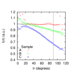
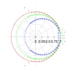
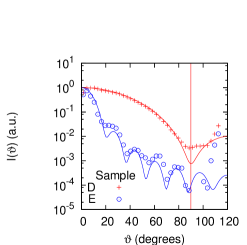
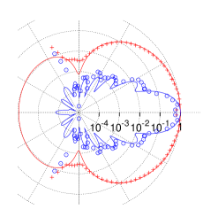
Fig. 7: Scattered intensity $I\left(\vartheta\right)$ measured as a function of the scattering angle $\vartheta$ in the plane perpendicular to the impinging polarization. Experimental results for polystyrene colloids A, B, C, D, E. The lines represent the values calculated with Mie theory for diameter $23\mathrm{nm}$, $81\mathrm{nm}$, $149\mathrm{nm}$, $450\mathrm{nm}$, and $1700\mathrm{nm}$ respectively. Left column graphs are in Cartesian coordinates, and right column graphs are in polar coordinates. Upper panels represent scattering intensity in linear scale, while in the lower panels the scale is logarithmic.

Continuous lines illustrate the exact Mie theoretical results [40]. For samples A, B, C (Fig. 7, upper panels) we compare the experimental data with the Mie theoretical values by using the diameters measured with dynamic SIFF and we obtain a reasonable agreement. For samples D and E the value of the particle diameter necessary for nicely fit the data is larger than the value obtained by dynamic SIFF, by an amount of about 12.5% and 5% respectively. The reason for this discrepancy is related to the difficulty inherent to low intensity measurements spanning more than two orders of magnitude. The vertical red line indicates the $90^{\circ}$ limit. The similarity with Mie theory confirms the ability of the proposed technique to measure the scattering signal up to angles of $90^{\circ}$ and beyond. We note that, in the present work, we are mainly interested in showing data at large angles, so we didn’t apply the necessary care to reduce the noise of the data at low angle (avoid convection, take larger statistical samples, extend the measurement over longer time spans, and other technicalities). Furthermode, systematic errors at low angles can be also introduced by the fact that low angle data are obtained by collecting light nearly along the impinging beam direction, corresponding to light entering at large angles into the objective, where aberrations are often present.

A further check of the capabilities of the technique has been obtained by measuring the $S\left(\vartheta\right)$ with two different polarizations of the impinging laser beam, i.e. parallel and perpendicular to the azimuthal angle $\varphi=0^{\circ}$. Fig. 8 shows the results obtained for the colloidal sample B, for both parallel (right panels) and perpendicular (left panels) components of the scattered light. The IPS are shown in the upper panels, while the corresponding $I\left(\vartheta\right)$ are shown in the lower panels. For the parallel case shown in the upper right panel, the dark bands in the corners represent the minimum of scattering intensity at $90^{\circ}$ along the polarization direction, a consequence of the dipolar radiation of the scatterers, showing the usual factor $\cos^{2}(\vartheta)$. The same feature can be observed in the corresponding $I\left(\vartheta\right)$ spectrum (lower right panel).

Fig. 8: Upper panels: Intensity Power Spectra IPS measured in two different polarization conditions. Lower panels: log-log polar plot of $I\left(\vartheta\right)$, along the diagonal ($\varphi=0$, red line). Left column: perpendicular component of scattering. Right column: parallel component of scattering. The spectra, for the parallel case, shows dark bands representing the minimum of scattering at $90^{\circ}$ along the polarization direction, due the dipolar scattering. Data obtained with sample B.

Fig. 9 shows the measured parallel and perpendicular scattering components $I\left(\vartheta\right)$, for two colloids B and C. Also in this case the data are compatible with the Mie theory, and one can easily detect the $90^{\circ}$ drop in the scattered intensity of the parallel component (blue dots in Fig. 9).

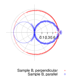
Fig. 9: Polar plots of the perpendicular and parallel components of the scattering intensity $I\left(\theta\right)$ measured as a function of the scattering angle $\vartheta$. Data obtained with colloidal samples B (left panel) and C (right panel). Intensity has been mapped as a square root, in order to emphasize the minima around $90^{\circ}$ of the parallel component.

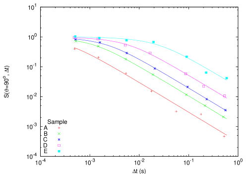
Fig. 10: Dynamic SINF measurements. Exposure-Time Dependent Spectra (ETDS), measured as a function of exposure time $\Delta t$, for $\vartheta=90^{\circ}$. Data obtained with samples A, B, C, D, E. Fitting lines are theoretical ETDS functions (see Eq. 6), with decay time $\tau=1/DQ^{2}$, and $D$ calculated with Stokes Einstein formula, using the values of nanoparticle diameters measured with dynamic SIFF and reported in Tab. 1.

Fig. 10 shows a log-log plot of the ETDS measured as a function of exposure time $\Delta t$, for $\vartheta=90^{\circ}$, for the different samples A, B, C, D, E. Fitting lines are theoretical ETDS functions (see Eq. 6), with decay time $\tau=1/DQ^{2}$, and $D$ calculated with Stokes Einstein formula. The data have been normalized so that the asymptotic value at short time is equal to 1. We have used in the ETDS function a value of the nanoparticle diameter as measured with dynamic SIFF and reported in Tab. 1. The expected dependence $f\left(\Delta t/\tau\right)$ is recognized. Also this experiment confirms that TLM allows detection of the scattered light at $90^{\circ}$.

8 Conclusions.

In the present paper, we have applied a new illumination geometry to a Scattering In the Near Field set up in order to increase the range of available scattering angles of the technique. The apparatus is based on a microscope equipped with a coherent source of light not collinear with the objective optical axis (Tilted Laser Microscopy). This enables measuring both the static and dynamic spectra of the sample up to backscattering angles ($110^{\circ}$), which was never achieved before with a SINF set up. The improvement of the wave vector range over the state-of-the-art [17] is of a factor 7, and 3.5 with respect to our experiments [12]. We introduced for the first time a non-trivial analysis algorithm necessary for extracting useful data. The data processing takes advantages of the ETDS approach to get access to time scales of the order of the camera minimum exposure time. The static and dynamic data have been compared with calibrated nanoparticles of various sizes in different polarization schemes.

9 Acknowledgements.

The authors are pleased to acknowledge fruitful discussion with F. Croccolo, C. Lancellotti and financial funding from EU (projects Bonsai LSHB–CT–2006–037639 and NAD CP–IP–212043–2).