Heating and cooling of magnetars with accreted envelopes

Abstract

We study the thermal structure and evolution of magnetars as cooling neutron stars with a phenomenological heat source in an internal layer. We focus on the effect of magnetized ($B\ga 10^{14}$ G) non-accreted and accreted outermost envelopes composed of different elements, from iron to hydrogen or helium. We discuss a combined effect of thermal conduction and neutrino emission in the outer neutron star crust and calculate the cooling of magnetars with a dipole magnetic field for various locations of the heat layer, heat rates and magnetic field strengths. Combined effects of strong magnetic fields and light-element composition simplify the interpretation of magnetars in our model: these effects allow one to interpret observations assuming less extreme (therefore, more realistic) heating. Massive magnetars, with fast neutrino cooling in their cores, can have higher thermal surface luminosity.

1 Introduction

We continue theoretical studies (Kaminker et al. 2006b, hereafter Paper I; also see Kaminker et al. 2006a, 2007) of persistent thermal activity of magnetar candidates – compact X-ray sources which include soft gamma repeaters (SGRs) and anomalous X-ray pulsars (AXPs). The magnetars are thought to be warm, isolated, slowly rotating neutron stars of age $t\lesssim 10^{5}$ yr with superstrong magnetic fields $B\gtrsim 10^{14}$ G (see, e.g., Woods & Thompson 2006, for a review). Following many authors (e.g., Colpi, Geppert & Page 2000; Thompson 2001; Pons et al. 2007), we assume that the high level of magnetar X-ray emission is supported by the release of the magnetic energy in their interiors. Although this assumption is widespread, there are alternative models (e.g., Chatterjee, Hernquist & Narayan 2000; Alpar 2001; Ertan et al. 2007; Thompson & Beloborodov 2005; Beloborodov & Thompson 2007).

In Paper I we studied the thermal evolution of magnetars as cooling isolated neutron stars with a phenomenological heat source in a spherical internal layer. We analyzed the location and power of the source and compared our calculations with observations of SGRs and AXPs. We showed that the heat source should be located at densities $\rho\lesssim 4\times 10^{11}$ ${\rm g\leavevmode\nobreak\ cm^{-3}}$, and the heating rate should be $\sim 10^{37}$ ${\rm erg\leavevmode\nobreak\ s^{-1}}$ to be consistent with the observational data and with the energy budget of isolated neutron stars. A deeper location of the heat source would be extremely inefficient to power the surface photon emission, because the heat would be carried away by neutrinos.

Here, we refine the model of the magnetar heat-blanketing envelope. In this envelope, the effects of superstrong magnetic fields are especially important. We analyze the blanketing envelope consisting not only of iron (Fe) but also of light elements (H or He) which can be provided by accretion at the early stage of magnetar evolution. Chemical composition and strong magnetic fields do affect thermal conduction in the blanketing envelope and the thermal structure of magnetars. In addition to the results of Paper I (and those of Potekhin & Yakovlev 2001 and Potekhin et al. 2003), we take into account neutrino energy losses in the outer crust of the neutron star, which can also be important (Potekhin, Chabrier & Yakovlev, 2007).

2 Observations

For the observational basis, we take seven sources: three SGRs and four AXPs listed in Table 1. We present their ages $t$, effective surface temperatures $T_{\mathrm{s}}^{\infty}$ (redshifted for a distant observer), and redshifted thermal luminosities $L_{\mathrm{s}}^{\infty}$. The estimates of spin-down ages $t$, blackbody effective surface temperatures $T_{\rm s}^{\infty}$, and non-absorbed thermal fluxes are taken from the SGR/AXP online Catalog maintained by the McGill Pulsar Group. All references in Table 1, except for Rho & Petre 1997 and Tiengo, Esposito & Mereghetti 2008, are taken from that Catalog. We do not include SGR 1627–41, the faint X-ray pulsar CXO J164710.2–455216 (e.g., Muno et al. 2006) and the unconfirmed AXP candidate AX J1845.0–0258 (e.g., Tam et al. 2006), because their ages $t$ are unknown (as well as the thermal luminosity $L_{\rm s}^{\infty}$ of SGR 1627–41). We also do not include two AXPs, XTE J1810–197 and 1E 1048.1–5937. Their high pulsed fractions ($\gtrsim 40\%$, e.g., Woods & Thompson 2006) indicate that their flux comes from a small fraction of the surface, incompatible with the model considered here. In addition, we have excluded the AXP 4U 0142+61 whose observed thermal emission can be attributed to a circumstellar dusty disk, rather than to a neutron star surface (Durant & Kerkwijk, 2006).

Table 1: Observational limits on ages $t$, effective surface temperatures $T_{\rm s}^{\infty}$, and blackbody luminosities $L_{\rm s}^{\infty}$ of magnetars

N	Source	$t$	$T_{\rm s}^{\infty}$	$\lg L_{\rm s}^{\infty}$	Refs.e)
		kyr	MK	erg s-1
1	SGR 1806–20	0.22	7.5${\pm 0.8}$	35.1  $\pm 0.4$	M00, M05
2	SGR 1900+14	1.1	5.0${\pm 0.6}$	34.9  $\pm 0.5$	W01
3	1E 1841–045	2.0 a)	5.1${\pm 0.2}$	35.15 $\pm 0.15$	VG97, M03
4	SGR 0526–66	5.0 a)	6.2${\pm 0.7}$	34.8  $\pm 0.4$	K03
5	CXOU J010043.1–721134	6.8	3.5$\pm 0.2$ b)	35.4 $\pm 0.2$ c)	T08
6	1RXS J170849.0–400910	9.0	5.3$\pm 0.1$	34.6 $\pm 0.1$	R05
7	1E 2259+586	19 a)	4.77$\pm 0.05$	34.4 $\pm 0.2$ d)	RP97, W04

^a) Ages of SNRs (see text for references)

^b) The soft component of the double blackbody (BB) spectral model (see text for details)

^c) Total BB luminosity of both components of the double spectral model

^d) From Eq. (1) with $D=3.0\pm 0.5$ kpc, the flux $f_{\rm thX}$ in the 2–10 keV energy band, and $\alpha_{\rm X}\sim 3.8$

^e) M00 – Mereghetti et al. (2000); M05 – Mereghetti et al. (2005); W01 – Woods et al. (2001); VG97 – Vasisht & Gotthelf (1997); M03 – Morii et al. (2003); K03 – Kulkarni et al. (2003); T08 – Tiengo et al. (2008); R05 – Rea et al. (2005); RP97 – Rho & Petre (1997); W04 – Woods et al. (2004)

In Fig. 1 we plot the blackbody surface luminosity $L_{\rm s}^{\infty}$ of the selected sources versus their ages. The current data are uncertain and our cooling models are too simplified to explain every source by its own cooling model. Instead, we will interpret magnetars as cooling neutron stars belonging to the “magnetar box,” the shaded rectangle in Fig. 1 (which reflects an average persistent thermal emission from magnetars, excluding bursting states).

Figure 1: Observational magnetar box (the shaded rectangle) of blackbody luminosity limits, $L_{\rm s}^{\infty}$ (see text and Table 1), of seven magnetars, supplemented by observational limits on $L_{\rm s}^{\infty}$ for eleven isolated neutron stars (marked by asterisks). The data are compared with theoretical cooling curves $L_{\rm s}^{\infty}(t)$ for a 1.1 $M_{\odot}$ neutron star with the dipole magnetic field $B_{\mathrm{p}}=5\times 10^{14}$ G (at the magnetic poles) and no internal heating, either without superfluidity (the solid line) or with strong proton superfluidity in the core (the dashed line SF).

The thermal luminosity limits $L_{\mathrm{s}}^{\infty}$ can be obtained as

$$L_{\mathrm{s}}^{\infty}=4\pi D^{2}f_{\mathrm{thX}}\alpha_{\rm X}.$$ (1)

Here, $f_{\mathrm{thX}}$ is a non-absorbed thermal flux detected from a source (in a certain $E_{1}$–$E_{2}$ X-ray energy band), $D$ is a distance to the source and

$$\alpha_{\rm X}=\frac{\pi^{4}}{15}\,\left(\int_{x_{1}}^{x_{2}}\frac{{\rm d}x\ x^{3}\ }{\exp(x)-1}\right)^{-1}$$ (2)

is the bolometric correction, with $x_{1,2}=E_{1,2}/k_{\rm B}T$. In particular, for the 2–10 keV band, we have $\alpha_{\rm X}\sim 2$–4. Thermal fluxes $f_{\mathrm{thX}}$ should be inferred from observations with account for the fractions BB/(PL+BB) of the blackbody (BB) components in the appropriate power law plus blackbody (PL+BB) spectral fits (references are listed in Table 1). The same fits provide the effective surface temperatures $T_{\mathrm{s}}^{\infty}$ and the apparent radii $R_{\mathit{BB}}^{\infty}$ of emitting regions. The radii are defined in such a way that

$$L_{\mathrm{s}}^{\infty}=4\pi\sigma(R_{\mathit{BB}}^{\infty})^{2}(T_{\rm s}^{\infty})^{4},$$ (3)

where $\sigma$ is the Stefan-Boltzmann constant. The radii $R_{\mathit{BB}}^{\infty}$ are typically smaller than the expected neutron star radii indicating that thermal emission can originate from some fraction of a neutron star surface. For instance, $R_{\mathit{BB}}^{\infty}\approx$2.4 and 5.5 km, for SGR 1806–20 and 1E 1841–045, respectively. Although the actual surface temperature may strongly vary within the emission region, spectral fits give a single (surface averaged) $T_{\mathrm{s}}^{\infty}$ value. The luminosities $L_{\mathrm{s}}^{\infty}$ in Table 1 and Fig. 1 are mainly obtained from Eq. (3) using the values of $T_{\mathrm{s}}^{\infty}$ and $R_{\mathit{BB}}^{\infty}$ presented in cited papers.

CXOU J010043.1–721134 is the only source from our collection, whose cumulative spectrum cannot be fit with a power-low plus blackbody model (Tiengo et al., 2008). Tiengo et al. (2008) fitted it by a sum of two blackbody components. The blackbody temperature of the softer component is given in Table 1. The radius of the corresponding emission region, $R_{BB}^{\infty}=12.1^{+2.1}_{-1.4}$ km, is comparable with the theoretical neutron star radius, although the pulsed fraction in the 0.2–6 keV energy range is rather high, $32\pm 3\%$. The harder component corresponds to $T_{{\rm s}2}^{\infty}=7.89\ ^{+1.05}_{-0.81}$ MK and $R_{\mathit{BB2}}^{\infty}=1.7\ ^{+0.6}_{-0.5}$ km, meaning probably a hot spot on the neutron star surface. We define the thermal luminosity $L_{\mathrm{s}}^{\infty}$ of this source as a sum of thermal luminosities of both blackbody components.

Radiation from five of the seven selected sources has the overall pulsed fraction $\lesssim 20\%$; the pulsed fraction for three of them is $\lesssim 10\%$ (e.g., Woods & Thompson 2006). This indicates that the thermal radiation can be emitted from a substantial part of the surface (although the pulsed fraction is lowered by the gravitational bending of light rays; e.g., Pavlov & Zavlin 2000 and references therein). Two other magnetars from Table 1, CXOU J010043.1–721134 and AXP 1RXS J170849.0–400910, have pulse fraction $\lesssim 40\%$ in the 0.5–2.0 keV band (e.g., Rea et al. 2005).

The majority of magnetar ages listed in Table 1 are characteristic spin down ages. For three sources, we adopt the ages of their host supernova remnants (SNRs): $t\sim 5$ kyr for SGR 0526–66 in SNR N49 (Kulkarni et al. 2003, also see Vancura et al. 1992); $t\sim 2$ kyr for 1E 1841–45 in SNR Kes 73 (Vasisht & Gotthelf, 1997); and $t\sim 19$ kyr for 1E 2259+586 in SNR CTB 109 (Rho & Petre, 1997). To specify the left and right boundaries of the magnetar box in Fig. 1, we introduce, somewhat arbitrarily, the uncertainties by a factor 2 into the ages $t$.

In our previous work we have compared simulations of magnetar cooling with the data on the effective surface temperature $T_{\mathrm{s}}^{\infty}$. Here, in contrast, we use the data on $L_{\rm s}^{\infty}$, which seem more robust. Note that explaining the data either on $T_{\mathrm{s}}^{\infty}$ or on $L_{\rm s}^{\infty}$ with our cooling models is not entirely self-consistent. According to observations of all sources, but CXOU J010043.1–721134, thermal emission originates from some fraction of the magnetar surface while our cooling models give thermal radiation from a large fraction of the surface. If we regarded (like in Paper I) the temperatures $T_{\mathrm{s}}^{\infty}$ given by spectral fits (see Table 1) as surface-averaged effective temperatures and calculated $L_{\rm s}^{\infty}$ using Eq. (3) with values of $R_{BB}^{\infty}$ realistic for neutron stars, we would obtain noticeably larger $L_{\rm s}^{\infty}$ than those provided by the observations (the magnetar box would raise in Fig. 1). On the contrary, matching the theory with the data on $L_{\rm s}^{\infty}$ (as in the present paper) gives lower surface-averaged temperatures $T_{\mathrm{s}}^{\infty}$ than the temperatures inferred from spectral fits.

We expect that the theory will be improved in the future by constructing more advanced models of magnetars – for instance, with highly nonuniform sources of internal energy release. On the other hand, current interpretation of magnetar observations is far from being perfect. It would be a challenge to construct new models of thermal radiation from strongly magnetized neutron stars and use them (rather than blackbody models) to interpret the data. In this case, by analogy with employing hydrogen atmosphere models for describing thermal radiation from ordinary neutron stars, we expect to get higher $R_{\mathit{BB}}$ (closer to the real neutron star radius) and lower $T_{\mathrm{s}}^{\infty}$. Moreover, thermal radiation emitted from a magnetar surface can be strongly distorted by magnetospheric effects (e.g., Lyutikov & Gavriil 2006; Rea et al. 2008). This can greatly complicate the problem of inferring $T_{\mathrm{s}}^{\infty}$ and $L_{\mathrm{s}}^{\infty}$ from the data.

Fig. 1 shows also observational limits $L_{\mathrm{s}}^{\infty}$ for eleven ordinary isolated neutron stars. The data are taken from Table 1 of Kaminker et al. (2006a) with a few changes described by Yakovlev et al. (2008). Following Slane et al. (2008) and Shibanov et al. (2008), we have enlarged the age range of the pulsar J0205+6449 (in the SNR 3C 58) to its characteristic age of 5.4 kyr. We have excluded one young and warm source, 1E 1207.4–5209, because of the problems of interpretation of its spectrum. We use the results of Ho et al. (2007) for the neutron star RX J1856.5–3754. The authors employed the magnetic hydrogen atmosphere model and obtained $T_{\rm s}^{\infty}=(4.34\pm 0.02)\times 10^{5}$ K and the apparent neutron star radius $R^{\infty}\approx 17$ km (at the 68$\%$ confidence level for the fixed distance $D=140$ pc). Taking into account a large scatter of distance estimates for RX J1856.5–3754 (Walter & Lattimer, 2002; van Kerkwijk & Kaplan, 2007), we have added 10% error bars to the latter values of $T_{\rm s}^{\infty}$.

Fig. 1 shows two typical cooling curves $L_{\mathrm{s}}^{\infty}(t)$ for a low-mass neutron star ($M=1.1\,M_{\odot}$) without internal heating and with a strong dipole magnetic field ($B_{\mathrm{p}}=5\times 10^{14}$ G at the magnetic poles). The solid line is for a non-superfluid star, while the dashed line SF assumes a strong proton superfluidity in the stellar core. This superfluidity suppresses neutrino emission in the core and thereby increases $L_{\mathrm{s}}^{\infty}$ at the neutrino cooling stage (e.g., Yakovlev & Pethick 2004).

Let us stress that the surface temperature of these stars is highly nonuniform; the magnetic poles are much hotter than the equator. In all figures we plot the total bolometric luminosity produced by the flux integrated over the stellar surface (e.g., Potekhin et al. 2003). The observations of ordinary neutron stars can be explained by the cooling theory without any reheating (e.g., Yakovlev & Pethick 2004; Yakovlev et al. 2008). The magnetars are much hotter (more luminous) than the ordinary cooling neutron stars; their observations imply that they have additional heat sources. As in Paper I, we assume that these sources are located inside magnetars.

3 Physics input

We have performed calculations with our cooling code (Gnedin, Yakovlev & Potekhin, 2001), which simulates the thermal evolution of an initially hot star via neutrino emission from the entire stellar body and via heat conduction to the surface and thermal photon emission from the surface. To facilitate calculations, the star is divided into the bulk interior and a thin outer heat-blanketing envelope (e.g., Gudmundsson, Pethick & Epstein 1983) which extends from the surface to the layer of the density $\rho=\rho_{\rm b}\sim 10^{10}-10^{11}$ ${\rm g\leavevmode\nobreak\ cm^{-3}}$; its thickness is a few hundred meters.

In the bulk interior ($\rho>\rho_{\rm b}$), the code solves the full set of thermal evolution equations in the spherically symmetric approximation. The standard version of the code neglects the effects of magnetic fields on thermal conduction and neutrino emission. In the present version, we have included neutrino-pair electron synchrotron radiation in a magnetic field $B$, that was neglected in Paper I.

In the blanketing envelope, the updated version of the code (see Potekhin et al. 2007, for details) uses a solution of stationary one-dimensional equations of hydrostatic equilibrium and thermal structure with radial heat transport, anisotropic temperature distribution, and a dipole magnetic field (Ginzburg & Ozernoĭ, 1964). It takes into account neutrino emission and possible heat sources in the envelope. The solution, applied to different parts of the envelope with locally constant magnetic fields, yields temperature profiles slowly varying from one part to another. For a given $T=T_{\rm b}$ at $\rho=\rho_{\rm b}$, we calculate the thermal flux emergent from different parts of the surface. Integrating it over the surface, we obtain the total photon luminosity $L_{\mathrm{s}}\equiv 4\pi\sigma R^{2}T_{\rm s}^{4}$, where $T_{\rm s}$ is the effective temperature properly averaged over the stellar surface and $R$ the circumferential neutron star radius. Redshifting then for a distant observer, we have $T_{\rm s}^{\infty}=T_{\rm s}\,\sqrt{1-r_{\rm g}/R}$ and $L_{\mathrm{s}}^{\infty}=(1-r_{\rm g}/R)\,L_{\mathrm{s}}$ ($r_{\mathrm{g}}=2GM/c^{2}$ being the Schwarzschild radius).

In the present calculations, we set either $\rho_{\rm b}=4\times 10^{11}$ ${\rm g\leavevmode\nobreak\ cm^{-3}}$ or (in the majority of cases) $\rho_{\rm b}=10^{10}$ ${\rm g\leavevmode\nobreak\ cm^{-3}}$ (see Sect. 4). We consider blanketing envelopes composed of ground-state or accreted matter. For the ground state matter, the composition is iron up to $\rho=10^{8}$ ${\rm g\leavevmode\nobreak\ cm^{-3}}$ and heavier elements (e.g., Haensel, Potekhin & Yakovlev 2007) at higher $\rho$ (it will be called the Fe composition). As an alternative, we have studied fully accreted envelopes composed successively of H, He, C, O up to maximum $\rho$ and $T$, where these elements can survive against pycno- or thermonuclear burning, and then the Fe composition (we use the same structure of the accreted envelope as in Potekhin et al. 2003). We have also considered accreted envelope models with H replaced by He, but found no significant difference.

An anisotropy of heat conduction, produced by strong magnetic fields, essentially modifies the temperature distribution in the blanketing envelope (which is included in our calculations). The anisotropy of heat conduction can also create anisotropic temperature distribution at $\rho>\rho_{\rm b}$, particularly, in the inner crust (that is not included in our code). Such situations should be simulated with a two-dimensional cooling code, as has been done by Geppert, Küker & Page (2004, 2006); Pérez-Azorín, Mirrales & Pons (2006) (for stationary cases) and most recently by Aguilera, Pons & Miralles (2008a, b, 2009); Pons, Miralles & Geppert (2009). The effect strongly depends on the values of thermal conductivity across the magnetic field. If one restricts oneself to the thermal conductivity of strongly degenerate electrons, the anisotropy of heat conduction (the ratio of thermal conductivities along and across the field) in a deep and not very hot magnetized crust can be huge (because of the strong magnetization of electrons which are mainly moving along magnetic field lines). However, in a hot crust (with increasing temperature) the electron magnetization and heat conduction anisotropy weaken. Moreover, the conductivity of phonons (lattice vibrations of Coulomb crystals of atomic nuclei; Chugunov & Haensel 2007) and vibrations of superfluid neutron liquid (superfluid phonons; Aguilera et al. 2009) in the inner crust can be much larger than the electron thermal conductivity across the field lines, washing out the temperature anisotropy and producing a nearly isotropic temperature distribution in the deep crust (although the electron conduction still dominates along field lines). This tendency is quite visible in recent calculations of Aguilera et al. (2009) and Pons et al. (2009) and justifies our approach.

At $T_{\rm b}\ga 10^{9}$ K the neutrino emission affects the thermal structure of the star. We calculate the neutrino emission in the crust (in the blanketing envelope and deeper) taking into account electron-positron pair annihilation, plasmon decay, neutrino bremsstrahlung in collisions of electrons with atomic nuclei, and synchrotron radiation of neutrino pairs by electrons (e.g., Yakovlev et al. 2001). The pair annihilation is relatively unimportant and can be neglected. Very strong magnetic fields in the outer crust of magnetars can modify the plasmon decay and bremsstrahlung neutrino processes. Such modifications have not been studied in detail; they can be important for the magnetar physics but are neglected here. Evidently, the synchrotron emission does depend on the magnetic field, which we take into account explicitly; it is important at $B\sim 10^{14}-10^{15}$ G (cf. Potekhin et al. 2007).

Following Paper I, we introduce an internal phenomenological heat source located in a spherical layer, $\rho_{1}<\rho<\rho_{2}$. The heat rate $H$ [${\rm erg\leavevmode\nobreak\ cm^{-3}\leavevmode\nobreak\ s^{-1}}$] is taken in the form

$$H=H_{0}\,\Theta(\rho)\,\exp(-t/\tau),$$ (4)

where $H_{0}$ is the maximum heat intensity, $\Theta\sim 1$ in a density interval $\rho_{1}<\rho<\rho_{2}$, and $\Theta$ vanishes outside this interval (at $\rho\ll\rho_{1}$ or $\rho\gg\rho_{2}$), $t$ is the star’s age, and $\tau$ is the e-folding decay time of the heat release. An exact shape of $\Theta(\rho)$ is unimportant for $T_{\rm s}$, provided that we fix the total heat power

$$W^{\infty}(t)=\int{\rm d}V\,{\rm e}^{2\Phi}\,H,$$ (5)

where ${\rm d}V$ is a proper volume element and $\Phi$ is the metric function that describes gravitational redshift. An illustration of this independence is given in Fig. 2, which displays temperature distributions in the crust for two different shapes of $\Theta(\rho)$. We see that a change of a shape of $\Theta(\rho)$ leaves almost intact the thermal structure at $\rho\ll\rho_{1}$ (and, therefore, it cannot affect thermal radiation).

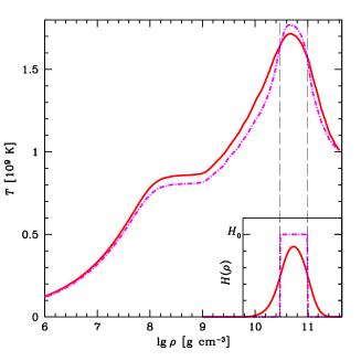
Figure 2: Temperature profiles along the magnetic axis of the neutron star with $M=1.4\,M_{\odot}$, $B=10^{15}$ G, $H_{0}=3\times 10^{20}$ ${\rm erg\leavevmode\nobreak\ cm^{-3}\leavevmode\nobreak\ s^{-1}}$, and two forms of the heat source profile, shown in the inset: smooth (solid lines) and piecewise-constant (dot-dashed lines).

Table 2: Five positions of the heat layer, and the heat power $W^{\infty}$ for the 1.4 $M_{\odot}$ star with $H_{0}=3\times 10^{20}$ ${\rm erg\leavevmode\nobreak\ cm^{-3}\leavevmode\nobreak\ s^{-1}}$ and $t=1$ kyr

No.	$\rho_{1}$ (${\rm g\leavevmode\nobreak\ cm^{-3}}$)	$\rho_{2}$ (${\rm g\leavevmode\nobreak\ cm^{-3}}$)	$W^{\infty}$ (erg s-1)
I	$3\times 10^{10}$	$10^{11}$	$4.0\times 10^{37}$
II	$10^{12}$	$3\times 10^{12}$	$1.9\times 10^{37}$
III	$3\times 10^{13}$	$10^{14}$	$1.1\times 10^{38}$
IV	$2\times 10^{10}$	$6\times 10^{10}$	$3.3\times 10^{37}$
V	$10^{11}$	$3\times 10^{11}$	$4.3\times 10^{37}$

According to Paper I, only the values $\tau\sim 10^{4}-10^{5}$ yr can be consistent with the magnetar box (Sect. 2). Longer $\tau$ would require too much energy (Sect. 5). In this paper, we take $\tau=5\times 10^{4}$ yr.

We employ the same EOS in the neutron star core as in Paper I. It is the model denoted as APR III by Gusakov et al. (2005); it is based on the EOS of Akmal, Pandharipande & Ravenhall (1998). According to this EOS, the core consist of nucleons, electrons, and muons. The maximum neutron star mass is $M=1.929\,M_{\odot}$. The powerful direct Urca process of neutrino emission (Lattimer et al., 1991) is allowed only in the central kernels of neutron stars with $M>1.685\,M_{\odot}$ (at densities $\rho>1.275\times 10^{15}$ ${\rm g\leavevmode\nobreak\ cm^{-3}}$).

We use two neutron star models, with $M=1.4\,M_{\odot}$ and $1.9\,M_{\odot}$. The former is an example of a star with the standard (not too strong) neutrino emission in the core (the modified Urca process in a non-superfluid star). In this case $R=12.27$ km and the central density is $\rho_{\rm c}=9.280\times 10^{14}$ ${\rm g\leavevmode\nobreak\ cm^{-3}}$. The latter model ($R=10.95$ km, $\rho_{\rm c}=2.050\times 10^{15}$ ${\rm g\leavevmode\nobreak\ cm^{-3}}$) gives an example of a star whose neutrino emission is enhanced by the direct Urca process in the inner core.

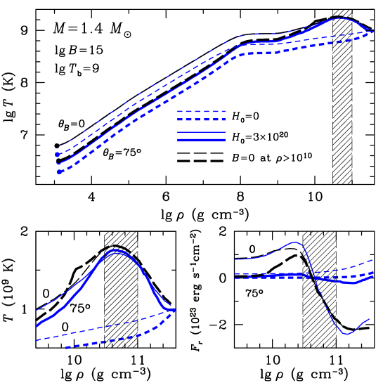
Figure 3: Temperature $T(\rho)$ and radial thermal flux $F(\rho)$ profiles in local parts of the outer crust of the 1.4$\,M_{\odot}$ neutron star (⁵⁶Fe envelope; $\rho_{\rm b}=4\times 10^{11}$ ${\rm g\leavevmode\nobreak\ cm^{-3}}$ and fixed $T_{\rm b}=10^{9}$ K) with a locally uniform magnetic field $B=10^{15}$ G directed at two angles $\theta_{B}$ to the surface normal, $\theta_{B}=0$ (thin lines) or $\theta_{B}=75^{\circ}$ (thick lines). The position of the heat layer (I in Table 2) is indicated by the shaded strips; the heat intensity is $H_{0}=3\times 10^{20}$ ${\rm erg\leavevmode\nobreak\ cm^{-3}\leavevmode\nobreak\ s^{-1}}$; solid lines – accurate calculations, long-dashed lines – magnetic field is off at $\rho>10^{10}$ ${\rm g\leavevmode\nobreak\ cm^{-3}}$; short-dashed lines – no heating, $H_{0}=0$. Top: entire temperature profiles at $\rho\leq\rho_{\rm b}$, the filled dots show the radiative surface (optical depth equals 2/3). Bottom: $T(\rho)$ in units of $10^{9}$ K (left) and $F(\rho)$ in units of $10^{23}$ erg cm^-2 s^-1 (right) in the vicinity of the heat layer.

Five examples of heat layer locations, $\rho_{1},\,\rho_{2}$, are given in Table 2. Three of them (I, II, and III) were used in Paper I. Let us remind that the outer crust has a thickness of a few hundred meters and a mass of $\sim 10^{-5}\,M_{\odot}$; the inner crust can be as thick as $\sim 1$ km and its mass is $\sim 10^{-2}\,M_{\odot}$, while the core has radius $\sim 10$ km and contains $\sim 99\%$ of the stellar mass. All five heat layers are relatively thin. The layers I, IV, and V are located in the outer crust; the layers II and III are at the top and bottom of the inner crust, respectively. For illustration, in Table 2 we present also the heat power $W^{\infty}$ calculated from Eq. (5) for the five layers in the $1.4\,M_{\odot}$ star of age $t=1000$ yr at $H_{0}=3\times 10^{20}$ ${\rm erg\leavevmode\nobreak\ cm^{-3}\leavevmode\nobreak\ s^{-1}}$.

4 Thermal structure of heat-blanketing envelopes

Fig. 3 shows the temperature and radial thermal flux profiles in local parts of the heat blanketing Fe envelope ($\rho\leq\rho_{\rm b}=4\times 10^{11}$ ${\rm g\leavevmode\nobreak\ cm^{-3}}$, $T_{\rm b}=10^{9}$ K) of the $1.4\ M_{\odot}$ star with a locally uniform magnetic field $B=10^{15}$ G directed at two angles to the surface normal, $\theta_{B}=0$ and $\theta_{B}=75^{\circ}$. One can compare the thermal structure of the blanketing envelope without heating (short-dashed lines; e.g., Potekhin et al. 2003, 2007) and with the heat source (solid lines) of the intensity $H_{0}=3\times 10^{20}$ ${\rm erg\leavevmode\nobreak\ cm^{-3}\leavevmode\nobreak\ s^{-1}}$, located in layer I (Table 2).

Long-dashed lines in Fig. 3 are obtained by solving the full set of one-dimensional equations for the blanketing envelope (Potekhin et al., 2007) including the heat source but with the magnetic field artificially switched off at $\rho>10^{10}$ ${\rm g\leavevmode\nobreak\ cm^{-3}}$. These calculations simulate the model used in Paper I, where a strongly magnetized blanketing envelope with $\rho_{\rm b}=10^{10}$ ${\rm g\leavevmode\nobreak\ cm^{-3}}$  was matched to the interior, in which the magnetic field effects were ignored. We see that at different $\theta_{B}$ the long-dashed $T(\rho)$ curves only slightly differ from the solid ones. Such a difference is more pronounced near the heat layer (the bottom left panel) but becomes invisible at lower $\rho$. We have obtained a significant difference only in a narrow range of field directions $\theta_{B}\approx 90^{\circ}$. However, in these cases the one-dimensional (radial) model becomes a poor approximation. The curvature of magnetic field lines in a more realistic model should increase the surface temperature in a narrow equatorial zone of width $\lesssim\sqrt{Rh}$ (along the surface), where $h$ is the thickness of the heat-blanketing envelope (Potekhin et al., 2007). An additional increase of the surface temperature in the above region can be provided by ion heat conduction (Chugunov & Haensel, 2007). The temperature raise will reduce the indicated difference between the solid and long-dashed lines.

We have obtained similar results for local radial heat flux $F(\rho)$ shown in the bottom-right panel of Fig. 3. The flux changes its sign inside the heat layer. The flux at $\rho\gtrsim 10^{11}$ ${\rm g\leavevmode\nobreak\ cm^{-3}}$ flows into the stellar interior, where the heat is radiated away by neutrinos (Paper I). The solid and long-dashed curves $F(\rho)$ are also indistinguishable at $\rho\lesssim 10^{10}$ ${\rm g\leavevmode\nobreak\ cm^{-3}}$. Calculations show that the convergence of two types of the curves is violated only at $B\gtrsim 10^{16}$ G.

We have verified that our calculations for the blanketing envelope with $\rho_{\rm b}=4\times 10^{11}$ ${\rm g\leavevmode\nobreak\ cm^{-3}}$ (including the heat layer) properly match those with $\rho_{\rm b}=10^{10}$ ${\rm g\leavevmode\nobreak\ cm^{-3}}$ (with the same heat layer being outside the blanketing envelope). These results justify the choice of the blanketing envelope with $\rho_{\rm b}=10^{10}$ ${\rm g\leavevmode\nobreak\ cm^{-3}}$ in our further calculations (at least with $B\lesssim 10^{15}$ G).

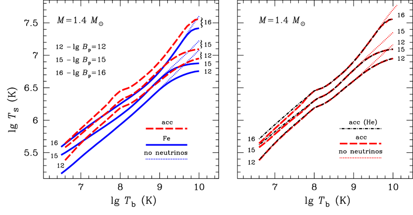
Figure 4: Surface temperature $T_{\rm s}$, averaged over the surface of the $M=1.4M_{\odot}$ neutron star, as a function of $T_{\rm b}$ for the blanketing envelope with $\rho_{\rm b}=10^{10}$ ${\rm g\leavevmode\nobreak\ cm^{-3}}$. Three families of curves 12, 15, and 16 correspond to the dipole magnetic fields with $B_{\mathrm{p}}=10^{12}$, $10^{15}$, and $10^{16}$ G, respectively. Left: Solid and dashed lines refer to the Fe and accreted envelopes; dotted lines are for the Fe envelopes neglecting neutrino emission. Right: Dashed lines – standard accreted envelopes; dash-and-dot lines ‘acc (He)’ – the accreted envelopes with hydrogen replaced by helium; dotted lines – standard accreted envelopes neglecting neutrino emission.

Fig. 4 shows the average surface temperature $T_{\rm s}$ of the $M=1.4M_{\odot}$ star versus $T_{\rm b}$. We assume a dipole magnetic field with $B_{\mathrm{p}}=10^{12}$, $10^{15}$, and $10^{16}$ at the magnetic poles. We consider our Fe and accreted envelopes as well as an accreted envelope with all hydrogen replaced by helium. One can see an appreciable increase of $T_{\rm s}$ with the growth of $B_{\mathrm{p}}$ above $10^{14}$ G because of the cumulative thermal conductivity enhancement. The most significant effect of the accreted envelopes is a systematic increase of $T_{\rm s}$ at any $T_{\rm b}$ with respect to the Fe envelope. The effect has been studied earlier (Potekhin, Chabrier & Yakovlev, 1997; Potekhin & Yakovlev, 2001; Potekhin et al., 2003). Here, we have verified that it is important for all magnetic fields $B_{\mathrm{p}}$ of our interest; it results from the thermal conductivity enhancement in large areas of the accreted envelope near the magnetic poles. More details on the $T_{\mathrm{b}}-T_{\mathrm{s}}$ relation for Fe envelopes are given in the Appendix.

The right panel in Fig. 4 shows that replacing hydrogen by helium in the accreted envelope at $T_{\rm b}\gtrsim 10^{8}$ K does not affect $T_{\rm s}$. The insensitivity of $T_{\rm s}$ to this replacement for non-magnetized neutron stars is known (Potekhin et al., 1997). Here, we have checked this property for magnetars. Only at $B_{\mathrm{p}}\gg 10^{14}$ G and relatively low temperatures $T_{\rm b}<10^{8}$ K the surface temperature $T_{\rm s}$ for the He envelope goes slightly higher. Generally, such an effect is unusual for ions with higher $Z$, which are better scatterer of electrons (cf. Potekhin et al. 1997, 2003). However, it occurs in the superstrong field because of deeper localization of the radiative surface for the He envelope, as a result of a lower energy plasma-frequency cutoff in the Rosseland opacity (Potekhin et al., 2003) for smaller $Z/A$. Anyway at $T_{\rm b}\gtrsim 10^{8}$ K replacing hydrogen by helium does not affect the thermal insulation of the blanketing envelope.

Also, Fig. 4 shows the effects of neutrino emission in the blanketing envelopes of different composition at $T_{\rm b}>10^{9}$ K. One can see that the neutrino emission limits the growth of $T_{\rm s}$ with increasing $T_{\rm b}$ (cf. Potekhin et al. 2007).

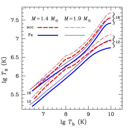
Figure 5: Average surface temperature $T_{\rm s}$ as a function of $T_{\rm b}$ for the $1.4M_{\odot}$ (thick lines) and $1.9M_{\odot}$ (thin lines) stars; solid and dashed lines refer to the same envelopes as in Fig. 4; labels 12 and 16 refer to the field strengths $B_{\mathrm{p}}=10^{12}$ and $10^{16}$ G.

Fig. 5 shows the dependence of $T_{\rm s}$ on $T_{\rm b}$ for the $1.4\,M_{\odot}$ and $1.9\,M_{\odot}$ stars with Fe and accreted envelopes. In a wide range of magnetic fields, we obtain systematically higher surface temperatures $T_{\rm s}$ (at the same $T_{\rm b}$) for the massive star as a result of smaller radius (see Sect. 3) and thinner blanketing envelope ($\Delta R_{\rm b}=R-R_{\rm b}\approx 170$ m for $M=1.4\,M_{\odot}$ versus $\Delta R_{\rm b}\approx 70$ m for $M=1.9M_{\odot}$). At a given $T_{\rm b}$, the surface temperature scales approximately as $T_{\rm s}\propto g^{1/4}$, where $g\approx GM/(R^{2}\sqrt{1-r_{\rm g}/R})$ is the surface gravity (e.g., Ventura & Potekhin 2001, and references therein).

5 Comparison with observations

A warm cooling neutron star with a powerful internal heating (Sect. 3) quickly (in $t\lesssim 10$ yr) reaches a quasi-stationary state regulated by the heat source. The energy is mainly carried away by neutrinos, but some fraction is transported by thermal conduction to the surface and radiated away by photons; the stellar interior stays highly non-isothermal. A thermal state of the heat source and outer layers is almost independent of the physics of deeper layers. This means the thermal decoupling of the heat source and outer layers from the deeper layers.

In general (Paper I) heating a warm neutron star from the core or the inner crust is inefficient for raising $T_{\rm s}$. With the increase of the heat power, $T_{\rm s}$ saturates because of the neutrino emission. Similar saturation of $T_{\rm s}$ by the neutrino emission was analyzed by Van Riper (1991) who studied thermal response of a neutron star to a steady-state heating. In Paper I we concluded that the heat source should be located in the outer crust in order to heat the surface and be consistent with the neutron star energy budget.

Figure 6: Left: Temperature dependence $T_{\mathrm{i}}(\rho)$ in the 1.4$\,M_{\odot}$ neutron star of age $t=1000$ yr with three different positions I, II, and III (Table 2) of the heat layer (hatched rectangles) and two levels of the heat intensity $H_{0}=3\times 10^{19}$ ${\rm erg\leavevmode\nobreak\ cm^{-3}\leavevmode\nobreak\ s^{-1}}$ and $3\times 10^{20}$ ${\rm erg\leavevmode\nobreak\ cm^{-3}\leavevmode\nobreak\ s^{-1}}$ for the Fe blanketing envelope and the dipole magnetic field with $B_{\mathrm{p}}=5\times 10^{14}$ G at the poles. In the upper part we indicate the density regions appropriate to the outer crust, inner crust and the core of the star. Right: Cooling curves in comparison with the magnetar box.

Fig. 6 is similar to Fig. 2 of Paper I. It is a reference figure for subsequent Figs. 7–9. The left panel of Fig. 6 shows the temperature profiles $T_{\mathrm{i}}(\rho)$ inside the 1.4 $M_{\odot}$ star of age $t=1000$ yr with the dipole magnetic field ($B_{\mathrm{p}}=5\times 10^{14}$ G). Here, $T_{\mathrm{i}}(\rho)=T(\rho)e^{\Phi}$ is the internal temperature redshifted for a distant observer, while $T(\rho)$ is the local temperature at a given $\rho$. It is $T_{\mathrm{i}}$ that is constant throughout thermally relaxed (isothermal) regions of the star in General Relativity. The same temperature $T_{\mathrm{i}}(\rho)$ has been plotted in Paper I and in Kaminker et al. (2007) (denoted there as $T(\rho)$). We consider three locations of the heat layer (I, II, and III in Table 2) and two intensities, $H_{0}=3\times 10^{19}$ and $3\times 10^{20}$ ${\rm erg\leavevmode\nobreak\ cm^{-3}\leavevmode\nobreak\ s^{-1}}$. In all the cases the stellar core is colder than the crust, because of intense neutrino cooling in the core. Pushing the heat source deeper into the crust we obtain a colder surface because of more efficient neutrino cooling.

The right panel of Fig. 6 shows cooling curves. Nearly horizontal parts of the curves at $t\lesssim\tau=5\times 10^{4}$ yr (Sect. 3) and their later sharp drops confirm that the surface thermal luminosity is solely maintained by internal heating. The initial parts ($t\lesssim 100$ yr) of two cooling curves for the heat layers II and III (at $H_{0}\sim 3\times 10^{19}$ ${\rm erg\leavevmode\nobreak\ cm^{-3}\leavevmode\nobreak\ s^{-1}}$) demonstrate the end of the relaxation to quasi-stationary thermal states. We can reconcile the cooling curves at lower heat intensity with more luminous sources in the magnetar box by placing the heat source in the outer crust. To minimize the energy consumption (see below) we employ the outer heat layer I in Figs. 7, 8 and the layers I, IV, and V in Fig.  9.

Figure 7: Left: Same as in the left panel of Fig. 6 but for one heat layer I, three heat intensities, and two magnetic fields ($B_{\mathrm{p}}=10^{14}$ – solid and long-dashed lines; and $B_{\mathrm{p}}=10^{15}$ G – dot-dashed and short-dashed lines). Solid and dot-dashed lines correspond to the Fe heat-blanketing envelope, dashed lines – to the accreted envelope; thick, intermediate, and thin lines are for the heat intensities $H_{0}=3\times 10^{18}$, $3\times 10^{19}$, and $3\times 10^{20}$ ${\rm erg\leavevmode\nobreak\ cm^{-3}\leavevmode\nobreak\ s^{-1}}$, respectively. Right: Cooling curves for these models.

The left panel in Fig. 7 shows the temperature profiles $T_{\mathrm{i}}(\rho)$ inside the 1.4 $M_{\odot}$ star of the age $t=1000$ yr with the heat source in layer I calculated for both the Fe and accreted blanketing envelopes. For comparison, we take three levels of the heat intensity, $H_{0}=3\times 10^{18}$ (thin lines), $H_{0}=3\times 10^{19}$ (intermediate lines), and $3\times 10^{20}$ ${\rm erg\leavevmode\nobreak\ cm^{-3}\leavevmode\nobreak\ s^{-1}}$ (thick lines), and two magnetic fields ($B_{\mathrm{p}}=10^{14}$ and $10^{15}$ G). The right panel in Fig. 7 demonstrates the appropriate cooling curves.

Under the heat-blanketing envelope (at $\rho>\rho_{\rm b}$), we take into account the magnetic field effects only by including the synchrotron neutrino radiation and (indirectly) the heat source that can be provided by magnetic fields. The synchrotron emissivity is calculated by putting $B=B_{\rm p}$. The neutrino synchrotron process in superstrong magnetic fields ($10^{14}-10^{15}$ G) lowers the temperature profiles in the stellar interior; this effect is more pronounced for stronger fields (cf. solid lines for $B_{\mathrm{p}}=10^{14}$ and dot-dashed lines for $B_{\mathrm{p}}=10^{15}$ G in the left panel of Fig. 7). The accreted matter in the blanketing envelope also reduces the temperature at $\rho\lesssim 10^{11}$ g cm^-3 because of higher heat transparency of the accreted envelope (higher heat flux to the surface).

Fig. 7 demonstrates that $L_{\mathrm{s}}^{\infty}$ is mainly regulated by the blanketing envelope. The combined effect of a superstrong magnetic field and an accreted envelope appreciably increases $L_{\mathrm{s}}^{\infty}$ (also see Fig. 4). The stronger heating ($H_{0}=3\times 10^{20}$ ${\rm erg\leavevmode\nobreak\ cm^{-3}\leavevmode\nobreak\ s^{-1}}$) at $B_{\rm p}=10^{15}$ G produces too warm magnetar envelope for any composition and gives larger $L_{\mathrm{s}}^{\infty}$ than required by the magnetar box. In a lower field, $B_{\rm p}=10^{14}$ G, the accreted envelope is also too warm but the Fe envelope is cooler and better consistent with the magnetar box. The weaker (intermediate) source ($H_{0}=3\times 10^{19}$ ${\rm erg\leavevmode\nobreak\ cm^{-3}\leavevmode\nobreak\ s^{-1}}$) also overheats the accreted envelopes at both $B_{\rm p}=10^{15}$ G and $B_{\rm p}=10^{14}$ G (intermediate short- and long-dashed lines); in this case the cooling curves for Fe envelopes better match the data. However, only the weakest chosen heat intensity ($H_{0}=3\times 10^{18}$ ${\rm erg\leavevmode\nobreak\ cm^{-3}\leavevmode\nobreak\ s^{-1}}$) is capable to cover the lower part of the magnetar box.

Figure 8: Same as in Fig. 7 but for the 1.9 $M_{\odot}$ star and two heat intensities $H_{0}=3\times 10^{19}$ (thin lines) and $3\times 10^{20}$ (thick lines).

Fig. 8 shows even more pronounced effects of the magnetar magnetic fields and accreted envelopes for the 1.9 $M_{\odot}$ star with two levels of heat intensities in the layer I. The left panel gives the temperature profiles $T_{\mathrm{i}}(\rho)$ at $\rho>\rho_{b}=10^{10}$ ${\rm g\leavevmode\nobreak\ cm^{-3}}$. They are noticeably lower than the corresponding profiles in the 1.4 $M_{\odot}$ star (because of the direct Urca process that operates in the inner core of the massive star). However, in the case of $H_{0}=3\times 10^{20}$ ${\rm erg\leavevmode\nobreak\ cm^{-3}\leavevmode\nobreak\ s^{-1}}$ the effect of the magnetized accreted envelope overrides that of the rapid neutrino cooling of the massive core (owing to thermal decoupling of the surface from the core). Comparing the right panels of Figs. 7 and 8, we see that at $H_{0}=3\times 10^{20}$ ${\rm erg\leavevmode\nobreak\ cm^{-3}\leavevmode\nobreak\ s^{-1}}$ and $t\lesssim 5\times 10^{4}$ yr the thermal luminosity of the heavier $1.9\,M_{\odot}$ star is higher than of the $1.4\,M_{\odot}$ star (because of higher $T_{\rm s}$, see Fig. 5), making the heavier star too hot. As discussed in Paper I, an intense heating in the outer crust of a massive star can outweigh fast neutrino cooling in the inner core. This effect is very unusual for ordinary cooling stars where massive stars are commonly colder than low-mass ones (e.g., Yakovlev & Pethick 2004).

In contrast, the effects of fast neutrino cooling in magnetars are more essential at $H_{0}=3\times 10^{19}$ ${\rm erg\leavevmode\nobreak\ cm^{-3}\leavevmode\nobreak\ s^{-1}}$. Tuning $H_{0}\sim(1-3)\times 10^{19}$ ${\rm erg\leavevmode\nobreak\ cm^{-3}\leavevmode\nobreak\ s^{-1}}$ and the chemical composition of the blanketing envelope, we can reasonably well explain the magnetar box. Note that the lowest heat intensity $H_{0}=3\times 10^{19}$ ${\rm erg\leavevmode\nobreak\ cm^{-3}\leavevmode\nobreak\ s^{-1}}$ taken in Fig. 8 is ten times larger than the lowest heat intensity $H_{0}=3\times 10^{18}$ ${\rm erg\leavevmode\nobreak\ cm^{-3}\leavevmode\nobreak\ s^{-1}}$ taken in Fig. 7, but the corresponding cooling curves do not strongly differ.

Figure 9: The effects of thermal conduction in the outer crust on the thermal evolution of the 1.4 $M_{\odot}$ star with the same magnetic field as in Fig. 6 at $H_{0}=3\times 10^{20}$ ${\rm erg\leavevmode\nobreak\ cm^{-3}\leavevmode\nobreak\ s^{-1}}$. Left: Temperature profiles in the star at $t=$1000 yr. The hatched rectangles show the positions of the heat layers I, IV, and V, and the layer (labeled as $\kappa_{\rm eff}=\kappa/10$), where the thermal conductivity is modified (see the text). Solid line is the same as in Fig. 6, thick short-dashed, long-dashed, and dot-dashed lines are for the thermal conductivity reduced by a factor of 10 and for the heat layers IV, I, and V, respectively; thin dashed line is for the thermal conductivity enhanced by a factor of $10^{3}$ and the heat layer I. Right: Cooling curves in comparison with the magnetar box.

Earlier we (Kaminker et al., 2007) have shown that strong variations of the thermal conductivity in the inner crust for the case of intense heating in layer I have no effect on the surface luminosity. Fig. 9 demonstrates the sensitivity of the thermal structure (the left panel) and cooling curves (the right panel) to artificial variations of the thermal conductivity in the outer crust. The left panel shows temperature profiles in the 1.4 $M_{\odot}$ 1000 yr-old star with the dipole magnetic field ($B_{\mathrm{p}}=5\times 10^{14}$ G) for three locations of the heat layer (cases I, IV, and V in Table 2) at $H_{0}=3\leavevmode\nobreak\ \times 10^{20}$ ${\rm erg\leavevmode\nobreak\ cm^{-3}\leavevmode\nobreak\ s^{-1}}$; the right panel gives respective cooling curves. The thick solid lines are the same as in Fig. 6. Other lines are calculated with the thermal conductivity modified in the density range $1.1\times 10^{10}\leq\rho\leq 4\times 10^{11}$ ${\rm g\leavevmode\nobreak\ cm^{-3}}$ (the range is marked in the left panel of Fig. 9 by a dot-hatched rectangle).

Thick dashed and dot-dashed lines are calculated with the thermal conductivity reduced by a factor of 10 ($\kappa_{\rm eff}=\kappa/10$). They illustrate a possible suppression of radial heat conduction (e.g., by a strong toroidal magnetic field in the outer crust). For the heat layers I (long-dashed lines) and IV (short-dashed lines) located closer to the bottom of the blanketing envelope, the conductivity reduction results in a sharper temperature drop inside the crust and in a cooler interior, with the tendency to the isothermal state. Taking the heat region V (thick dot-dashed lines), shifted to the inner edge of the layer with the reduced conductivity, we obtain qualitatively the same behavior of $T_{\mathrm{i}}(\rho)$, as in the cases II and III in Fig. 6. The thermal energy easier flows inside the star than in the case I with normal conduction (solid lines).

On the contrary, the enhanced thermal conductivity (thin dashed lines) produces a wide quasi-isothermal layer in the outer crust (the left panel of Fig. 9) and a photon surface luminosity (the right panel) that is nearly the same, as for the normal conductivity (the thick solid line). In other words, $L_{\mathrm{s}}^{\infty}(t)$ is slightly sensitive to a conductivity increase. Comparing the right panels of Figs. 9 and 7 (thick lines), we conclude that a conductivity increase at $\rho>\rho_{\rm b}$ is incapable to rise $L_{\mathrm{s}}^{\infty}$, while an increase at $\rho<\rho_{\rm b}$ can rise it.

Finally, let us discuss briefly the energy budget of magnetars. Following Paper I, we assume that the maximum energy of the internal heating is $E_{\rm max}\sim 10^{50}$ erg (which is the magnetic energy of the star with $B\sim 3\times 10^{16}$ G in the core). Then the maximum persistent energy generation rate is $W_{\rm max}\sim E_{\rm max}/\tau\sim 3\times 10^{37}$ erg s^-1. For example, let us take an 1.4$\,M_{\odot}$ neutron star of age $t\ll\tau$ with the heat source in layer I. For an intense heating with $H_{0}\sim 3\times 10^{20}$ ${\rm erg\leavevmode\nobreak\ cm^{-3}\leavevmode\nobreak\ s^{-1}}$ we obtain $W^{\infty}\sim W_{\mathrm{max}}$ (and, therefore, $H_{0}$ cannot be larger). For a less intense heating with $H_{0}\sim 3\times 10^{19}$ ${\rm erg\leavevmode\nobreak\ cm^{-3}\leavevmode\nobreak\ s^{-1}}$ we have a more relaxed condition $W^{\infty}\sim 0.1\,W_{\mathrm{max}}$ (which would leave some energy for bursting activity of magnetars).

It follows from Figs. 6–9, that the heating should be sufficiently intense to keep $L_{\mathrm{s}}^{\infty}$ on the magnetar values ($\sim 10^{35}$ erg s^-1). However, for realistic magnetic fields $B\sim(2-10)\times 10^{14}$ G, the maximum allowable heat intensity $H_{0}\sim 3\times 10^{20}$ ${\rm erg\leavevmode\nobreak\ cm^{-3}\leavevmode\nobreak\ s^{-1}}$ and accreted envelopes, we have the thermal surface luminosity $L_{\mathrm{s}}^{\infty}\sim 10^{36}$ erg s^-1, noticeably higher than the luminosity of magnetars (Fig. 7). For Fe envelopes and the same heat intensity, we obtain $L_{\mathrm{s}}^{\infty}\gtrsim 3\times 10^{35}$ erg s^-1, consistent with the upper part of the magnetar box but giving the stringent energy budget ($W^{\infty}\sim W_{\mathrm{max}}$). Using a weaker heat intensity $H_{0}\sim 3\times 10^{19}$ ${\rm erg\leavevmode\nobreak\ cm^{-3}\leavevmode\nobreak\ s^{-1}}$ and accreted envelopes, we obtain still greater thermal luminosity $L_{\mathrm{s}}^{\infty}>4\times 10^{35}$ erg s^-1, which is too high for the magnetar box but provides a reasonable energy budget. Finally, varying weaker heating rate $H_{0}\lesssim 10^{19}$ ${\rm erg\leavevmode\nobreak\ cm^{-3}\leavevmode\nobreak\ s^{-1}}$ and the chemical composition of the blanketing envelope (Fig. 7) we have the luminosity $L_{\mathrm{s}}^{\infty}\sim 10^{35}$ erg s^-1, that is consistent with the magnetar box.

Accordingly, the presence of accreted envelopes simplifies the explanation of magnetars as cooling neutron stars (in our model). Our results show that we can reconcile the theory with observations assuming the accreted envelopes and lower heat intensities, $H_{0}\sim 10^{19}$ ${\rm erg\leavevmode\nobreak\ cm^{-3}\leavevmode\nobreak\ s^{-1}}$. Note that in all the cases the efficiency of heat conversion into the thermal radiation, $L_{\mathrm{s}}^{\infty}/W^{\infty}$, is low but the accreted envelopes increase it. For instance, assuming $H_{0}\sim 3\times 10^{19}$ ${\rm erg\leavevmode\nobreak\ cm^{-3}\leavevmode\nobreak\ s^{-1}}$ we have $L_{\mathrm{s}}^{\infty}/W^{\infty}\sim 0.01$ for Fe envelopes and $L_{\mathrm{s}}^{\infty}/W^{\infty}\sim 0.1$ for accreted ones.

6 Conclusions

We have analyzed the hypothesis that magnetars are isolated neutron stars with $B\gtrsim 10^{14}$ G, heated by a source localized in an internal layer. We have modelled the thermal evolution of magnetars, taking into account that their heat blanketing envelopes can be composed of light elements. Such envelopes can appear either due to a fallback accretion after a supernova explosion (e.g., Chevalier 1989, 1996; Chang, Arras & Bildsten 2004), probably with subsequent nuclear spallation reactions (Bildsten, Salpeter & Wasserman, 1992), or due to later and more prolonged accretion from a fossil disk (e.g., Chatterjee et al. 2000; Wang, Chakrabarty & Kaplan 2006; Ertan et al. 2007; Romanova, Kulkarni & Lovelace 2008) or from the interstellar medium (e.g., Nelson, Salpeter, & Wasserman 1993; Morley 1996).

Compared to Paper I, we have (i) included the effects of accreted envelopes, and (ii) changed the strategy of reconciling the theory with observations. We rely now on observational limits of quasi-persistent thermal luminosities of magnetars; this lowers the magnetar box (Sect. 2) and relaxes theoretical constraints on the properties of internal heat sources.

The main conclusions are as follows:

(1) The presence of light elements in the outer envelope of a magnetized neutron star can significantly increase the thermal conductivity and the thermal stellar luminosity $L_{\mathrm{s}}^{\infty}$ (for a given temperature $T_{\rm b}$ at the bottom of the heat blanketing envelope). Similar conclusions have been made earlier for ordinary cooling neutron stars with $B\lesssim 10^{13}$ G (Potekhin et al. 1997; Yakovlev & Pethick 2004, and references therein) as well as for strongly magnetized cooling stars (e.g., Potekhin et al. 2003).

(2) The luminosity $L_{\mathrm{s}}^{\infty}$ of the star with an accreted envelope is insensitive to replacing all accreted hydrogen by helium (as in ordinary neutron stars, see Potekhin et al. 1997). In particular, these results can be used for taking into account rapid nuclear burning of hydrogen and accumulation of helium in the outer part of the envelope (e.g., Chang et al. 2004).

(3) The combined effect of a superstrong magnetic field and an accreted envelope simplifies the interpretation of observations of quasi-persistent thermal radiation from magnetars using our model. We confirm the conclusion of Paper I that the our most favorable models require the heat source to be located in the outer crust (at $\rho\lesssim 4\times 10^{11}$ ${\rm g\leavevmode\nobreak\ cm^{-3}}$). However, the presence of accreted envelopes allows us to take lower heat intensities $H_{0}\sim 10^{19}$ ${\rm erg\leavevmode\nobreak\ cm^{-3}\leavevmode\nobreak\ s^{-1}}$ and place the heat layer slightly deeper in the stellar interior.

(4) In accordance with Paper I, in all our successful models (with and without accreted envelopes), heating of the outer crust produces a strongly nonuniform temperature distribution within the star. The temperature in the heat layer exceeds $10^{9}$ K, while the bottom of the crust and the stellar core remain much colder. The outer crust is thermally decoupled from the inner layers; thermal surface emission is rather insensitive to the properties of the inner layers (such as the EOS, neutrino emission, thermal conductivity, superfluidity of baryons).

(5) The surface thermal luminosity is weakly affected by variations of the thermal conductivity in the outer crust below the heat blanketing envelope. Therefore, the effects of the magnetic field on the conductivity in the heat layer cannot greatly change the surface luminosity. The thermal surface radiation is mainly regulated by the heat source as well as by the magnetic field and chemical composition of the blanketing envelope. Nevertheless, our calculations can be improved by a more careful treatment of heat transport in the entire magnetized outer crust, at $\rho\gtrsim 10^{10}$ ${\rm g\leavevmode\nobreak\ cm^{-3}}$, with different magnetic field configurations (e.g., Geppert et al. 2006; Aguilera et al. 2008a).

(6) Increasing the surface thermal emission of the star, which has a relatively high heat intensity ($H_{0}\sim 10^{20}$ ${\rm erg\leavevmode\nobreak\ cm^{-3}\leavevmode\nobreak\ s^{-1}}$) and an accreted envelope, is even more efficient if the star is massive (and possesses, therefore, thinner and more heat transparent crust). This effect is stronger than fast neutrino cooling due to direct Urca process that can be allowed in the core of a massive star.

(7) The presence of an accreted envelope can raise the efficiency of heat conversion into the surface radiation. It can become as high as $\sim 10\%$ (compared to a maximum of $\sim 1$% for Fe envelopes). This enables us to make our models more consistent with the total energy budget of heat sources in a neutron star. Now we can reduce the total energy to $E_{\rm tot}^{\infty}\sim 10^{48}-10^{49}$ erg (instead of the previously assumed level of $E_{\rm tot}^{\infty}\sim 10^{49}-10^{50}$ erg).

Further observations as well as new models of magnetar atmospheres are needed for more reliable interpretation of observations. The physics of internal heating is still not clear; it should be elaborated in the future.

Appendix A $T_{\mathrm{b}}$ – $T_{\mathrm{s}}$ relation

Table 3: Internal temperature $T_{\mathrm{b}}$ [K] together with effective surface temperature $T_{\mathrm{s}}$ [K] and internal outward heat flux $F_{\mathrm{b}}$ [erg s^-1 cm^-2] (either at the magnetic pole or surface averaged, av) for a 1.4 $M_{\odot}$ neutron star of radius $R$=12.27 km with the Fe envelope at $B_{\mathrm{p}}=10^{12}$ G and $\rho_{\mathrm{b}}=10^{10}$ ${\rm g\leavevmode\nobreak\ cm^{-3}}$.

$\lg T_{\mathrm{b}}$	$\lg T_{\mathrm{s}}$	$\lg F_{\mathrm{b}}$	$\lg T_{\mathrm{s}}$	$\lg F_{\mathrm{b}}$
	pole	pole	av	av
6.8	5.38	17.29	5.31	17.02
7.0	5.49	17.73	5.42	17.45
7.2	5.60	18.17	5.52	17.87
7.4	5.70	18.58	5.62	18.27
7.6	5.80	18.98	5.72	18.67
7.8	5.90	19.37	5.82	19.07
8.0	6.00	19.77	5.92	19.47
8.2	6.10	20.17	6.03	19.89
8.4	6.20	20.58	6.13	20.31
8.6	6.31	21.01	6.24	20.76
8.8	6.41	21.46	6.36	21.27
9.0	6.51	22.10	6.47	22.02
9.2	6.61	22.92	6.57	22.90
9.4	6.68	23.67	6.65	23.67
9.6	6.74	24.34	6.72	24.34
9.8	6.79	24.97	6.77	24.97

Table 4: Same as in Table 3 but for $B_{\mathrm{p}}=10^{15}$ G.

$\lg T_{\mathrm{b}}$	$\lg T_{\mathrm{s}}$	$\lg F_{\mathrm{b}}$	$\lg T_{\mathrm{s}}$	$\lg F_{\mathrm{b}}$
	pole	pole	av	av
6.8	5.66	18.44	5.58	18.09
7.0	5.74	18.76	5.65	18.40
7.2	5.82	19.08	5.73	18.72
7.4	5.91	19.40	5.81	19.04
7.6	5.99	19.72	5.90	19.36
7.8	6.07	20.05	5.98	19.69
8.0	6.15	20.39	6.06	20.04
8.2	6.24	20.75	6.16	20.41
8.4	6.34	21.16	6.26	20.83
8.6	6.46	21.61	6.38	21.30
8.8	6.58	22.12	6.50	21.81
9.0	6.71	22.68	6.62	22.37
9.2	6.82	23.36	6.73	23.04
9.4	6.90	24.10	6.81	23.77
9.6	6.96	24.82	6.86	24.47
9.8	6.98	25.53	6.89	25.21

Table 5: Same as in Table 3 but for $\rho_{\mathrm{b}}=4\times 10^{11}$ ${\rm g\leavevmode\nobreak\ cm^{-3}}$.

$\lg T_{\mathrm{b}}$	$\lg T_{\mathrm{sp}}$	$\lg F_{\mathrm{bp}}$	$\lg T_{\mathrm{s}}$	$\lg F_{\mathrm{b}}$
	pole	pole	av	av
6.8	5.37	17.32	5.31	17.05
7.0	5.49	17.77	5.42	17.49
7.2	5.59	18.20	5.52	17.91
7.4	5.70	18.61	5.62	18.31
7.6	5.80	19.01	5.72	18.70
7.8	5.89	19.40	5.82	19.10
8.0	5.99	19.80	5.92	19.50
8.2	6.09	20.20	6.02	19.91
8.4	6.19	20.60	6.13	20.33
8.6	6.30	21.02	6.23	20.78
8.8	6.40	21.53	6.34	21.39
9.0	6.47	22.46	6.43	22.45
9.2	6.50	23.64	6.46	23.64
9.4	6.51	24.76	6.46	24.77
9.6	6.51	25.67	6.46	25.67
9.8	6.51	26.41	6.46	26.41

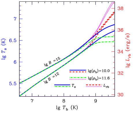
Figure 10: The surface-averaged effective temperature $T_{\mathrm{s}}$ (left vertical axis, solid and dot-dashed lines) and the total heat flux $L_{\mathrm{rb}}$ through the inner boundary of the Fe blanketing envelope (right vertical axis, dashed and dotted lines) in the 1.4 $M_{\odot}$ star for $\rho_{\mathrm{b}}=10^{10}$ ${\rm g\leavevmode\nobreak\ cm^{-3}}$ (solid and dashed lines) and $\rho_{\mathrm{b}}=4\times 10^{11}$ ${\rm g\leavevmode\nobreak\ cm^{-3}}$ (dot-dashed and dotted lines), for $B=10^{12}$ G (lower curve of each pair) and $10^{15}$ G (upper curves).

In Tables 3–5 we present the relations between the temperature $T_{\mathrm{b}}$ at the inner boundary of the blanketing envelope ($\rho=\rho_{\mathrm{b}}$) and the non-redshifted effective surface temperature $T_{\mathrm{s}}$. In addition, we list the values of the outward radial heat flux $F_{\mathrm{b}}$ at $\rho=\rho_{\mathrm{b}}$. We assume no heat sources in the envelope and consider the Fe envelope in the 1.4 $M_{\odot}$ neutron star of radius $R=12.27$ km with the dipole magnetic field ($B_{\mathrm{p}}=10^{12}$ or $10^{15}$ G at the magnetic pole). We present local values of $T_{\mathrm{s}}$ and $F_{\mathrm{b}}$ at magnetic poles, as well as surface-averaged values (av).

Table 3 refers to $B_{\mathrm{p}}=10^{12}$ G and $\rho_{\mathrm{b}}=10^{10}$ ${\rm g\leavevmode\nobreak\ cm^{-3}}$; Table 4 to $B_{\mathrm{p}}=10^{15}$ G and $\rho_{\mathrm{b}}=10^{10}$ ${\rm g\leavevmode\nobreak\ cm^{-3}}$; and Table 5 to $B_{\mathrm{p}}=10^{12}$ G and $\rho_{\mathrm{b}}=4\times 10^{11}$ ${\rm g\leavevmode\nobreak\ cm^{-3}}$.

Fig. 10 compares these $T_{\mathrm{b}}$ – $T_{\mathrm{s}}$ relations. We see that $T_{\mathrm{s}}$ saturates at $T_{\mathrm{b}}\gtrsim 10^{9}$ K if $\rho_{\mathrm{b}}$ is placed at the bottom of the outer crust, $\rho_{\mathrm{b}}=4\times 10^{11}$ ${\rm g\leavevmode\nobreak\ cm^{-3}}$, but it does not saturate at lower $\rho_{\mathrm{b}}=10^{10}$ ${\rm g\leavevmode\nobreak\ cm^{-3}}$. In the former case the saturation occurs because of the strong neutrino emission at $\rho_{\mathrm{b}}\gtrsim 10^{10}$ ${\rm g\leavevmode\nobreak\ cm^{-3}}$ and high temperatures. We also plot the total outward heat flux through the boundary of the blanketing envelope, $L_{\mathrm{rb}}$, in such a scale that corresponding curves match the $T_{\mathrm{b}}$ – $T_{\mathrm{s}}$ curves at low $T_{\mathrm{b}}$. Then, the deviation of the $T_{\mathrm{s}}$-curves from the $L_{\mathrm{rb}}$-curves directly measures the total energy loss due to neutrino emission in the blanketing envelope (at $\rho<\rho_{\mathrm{b}}$).

References

- Aguilera et al. (2008a) Aguilera D.N., Pons J.A., Miralles J.A., 2008a, A&A, 486, 255
- Aguilera et al. (2008b) Aguilera D.N., Pons J.A., Miralles J.A., 2008b, ApJ, 673, L167.
- Aguilera et al. (2009) Aguilera D.N., Cirigliano V., Pons J.A., Reddy S., Sharma R., 2009, Phys. Rev. Lett., submitted [arXiv:0807.4754].
- Akmal et al. (1998) Akmal A., Pandharipande V.R., Ravenhall D.G., 1998, Rhys. Rev., C58, 1804
- Alpar (2001) Alpar M.A., 2001, ApJ, 554, 1245
- Beloborodov & Thompson (2007) Beloborodov A.M., Thompson C., 2007, ApJ, 657, 967
- Bildsten et al. (1992) Bildsten L., Salpeter E.E., Wasserman I., 1992, ApJ, 384, 143
- Chatterjee et al. (2000) Chatterjee P., Hernquist L., Narayan R., 2000, ApJ, 534, 373
- Chang et al. (2004) Chang P., Arras P., Bildsten L., 2004, ApJ, 616, L147
- Chevalier (1989) Chevalier R.A., 1989, ApJ, 346, 847
- Chevalier (1996) Chevalier R.A., 1996, ApJ, 459, 322
- Chugunov & Haensel (2007) Chugunov A.I., Haensel P., 2007, MNRAS, 381, 1143
- Colpi et al. (2000) Colpi M., Geppert U., Page D., 2000, ApJ, 529, L29
- Durant & Kerkwijk (2006) Durant M., van Kerkwijk M.H., 2006, ApJ, 650, 1082
- Ertan et al. (2007) Ertan Ü., Alpar M.A., Erkut M.H., Ekşi K.Y., Çalişkan Ş., 2007, Ap&SS, 308, 73
- Geppert et al. (2004) Geppert U., Küker M., Page D., 2004, A&A, 426, 267
- Geppert et al. (2006) Geppert U., Küker M., Page D., 2006, A&A, 457, 937
- Ginzburg & Ozernoĭ (1964) Ginzburg V.L., Ozernoĭ L.M., 1964, Zh. Eksp. Teor. Fiz., 47, 1030 (English translation: Sov. Phys.-JETP, 20, 689)
- Gnedin et al. (2001) Gnedin O.Y., Yakovlev D.G., Potekhin A.Y., 2001, MNRAS, 324, 725
- Gudmundsson et al. (1983) Gudmundsson E.H., Pethick C.J., Epstein R.I., 1983, ApJ, 272, 286
- Gusakov et al. (2005) Gusakov M.E., Kaminker A.D., Yakovlev D.G., Gnedin O.Y., 2005, MNRAS, 363, 555
- Haensel et al. (2007) Haensel P., Potekhin A.Y., Yakovlev, D.G., 2007, Neutron Stars 1: Equation of State and Structure. Springer, New York
- Ho et al. (2007) Ho W.C.G., Kaplan D.L., Chang P., van Adelsberg M., Potekhin A.Y., 2007, MNRAS, 375, 821
- Kaminker et al. (2006a) Kaminker A.D., Gusakov M.E., Yakovlev D.G., Gnedin O.Y., 2006a, MNRAS, 365, 1300
- Kaminker et al. (2006b) Kaminker A.D., Yakovlev D.G., Potekhin A.Y., Shibazaki N., Sthernin P.S., Gnedin O.Y., 2006b, MNRAS, 371, 477 (Paper I)
- Kaminker et al. (2007) Kaminker A.D., Yakovlev D.G., Potekhin A.Y., Shibazaki N., Sthernin P.S., Gnedin O.Y., 2007, Ap&SS, 308, 423
- Kulkarni et al. (2003) Kulkarni S.R., Kaplan D.L., Marshall H.L., Frail D.A., Murakami T., Yonetoku D., 2003, ApJ, 585, 948
- Lattimer et al. (1991) Lattimer J.M., Pethick C.J., Prakash M., Haensel P., 1991, Phys. Rev. Lett., 66, 2701
- Lyutikov & Gavriil (2006) Lyutikov M., Gavriil F.P., 2006, MNRAS, 368, 690
- Mereghetti et al. (2000) Mereghetti S., Cremonesi D., Feroci M., Tavani M., 2000, A&A, 361, 240
- Mereghetti et al. (2005) Mereghetti S., Tiengo A., Esposito P., Götz D., Stella L., Israel G.L., Rea N., Feroci M., Turolla R., Zane S., 2005, ApJ, 628, 938
- Morii et al. (2003) Morii M., Sato R., Kataoka J., Kawai N., 2003, PASJ, 55, L45
- Morley (1996) Morley P.D., 1996, A&A, 313, 204
- Muno et al. (2006) Muno M.P., Clark J.S., Crowther P.A., Dougherty S.M., de Grijs R., Law C., McMillan S.L.W., Morris M.R., Negueruela I., Pooley D., Zwart S.P., Yusef-Zadeh F., 2006, ApJ, 636, L41
- Nelson et al. (1993) Nelson R.W., Salpeter E.E., Wasserman I., 1993, ApJ, 418, 874
- Pavlov & Zavlin (2000) Pavlov G.G., Zavlin V.E., 2000, ApJ, 529, 1011
- Pérez-Azorín et al. (2006) Pérez-Azorín J.F., Miralles J.A., Pons J.A., 2006, A&A, 451, 1009
- Pons et al. (2007) Pons J.A., Link B., Miralles J.A., Geppert U., 2007, Phys. Rev. Lett., 98, 071101
- Pons et al. (2009) Pons J.A., Miralles J.A., Geppert U., 2009, A&A, accepted [arXiv:0812.3018v1].
- Potekhin & Yakovlev (2001) Potekhin A.Y., Yakovlev D.G., 2001, A&A, 374, 213
- Potekhin et al. (1997) Potekhin A.Y., Chabrier G., Yakovlev D.G., 1997, A&A, 323, 415
- Potekhin et al. (2003) Potekhin A.Y., Yakovlev D.G., Chabrier G., Gnedin O.Y., 2003, ApJ, 594, 404
- Potekhin et al. (2007) Potekhin A.Y., Chabrier G., Yakovlev D.G., 2007, Ap&SS, 308, 353 (electronic version with corrected misprints: arXiv:astro-ph/0611014v3)
- Rea et al. (2005) Rea N., Oosterbroek T., Zane S., Turolla R., Méndez M., Israel G.L., Stella L., Haberl F., 2005, MNRAS, 361, 710
- Rea et al. (2008) Rea N., Zane S., Turolla R., Lyutikov M., Götz D., 2008, ApJ, 686, 1245
- Rho & Petre (1997) Rho J., Petre R., 1997, ApJ, 484, 828
- Romanova et al. (2008) Romanova M.M., Kulkarni A.K., Lovelace R.V.E., 2008, ApJ, 673, L171
- Shibanov et al. (2008) Shibanov Yu.A., Lundqvist N., Lundqvist P., Sollerman J., Zyuzin D., 2008, A&A, 486, 273
- Slane et al. (2008) Slane P., Helfand D.J., Reynolds S.P., Gaensler B.M., Lemiere A., Wang Z., 2008, ApJ, 676, L33
- Tam et al. (2006) Tam C.R., Kaspi V.M., Gaensler B.M., Gotthelf E.V., 2006, ApJ, 652, 548
- Thompson (2001) Thompson C., 2001, in Kouveliotou C., Ventura J., Van den Heuvel E., eds, The Neutron Star – Black Hole Connection, NATO Science Ser. C, vol. 567. Kluwer, Dordrecht, p. 369
- Thompson & Beloborodov (2005) Thompson C., Beloborodov A.M., 2005, ApJ, 634, 565
- Tiengo et al. (2008) Tiengo A., Esposito P., Mereghetti S., 2008, ApJ, 680, L133
- Vancura et al. (1992) Vancura O., Blair W.P., Long K.S., Raymond J.C., 1992, ApJ, 394, 158
- Van Riper (1991) Van Riper K., 1991, ApJ, 372, 251
- van Kerkwijk & Kaplan (2007) van Kerkwijk M.H., Kaplan D.L., 2007, Ap&SS, 308, 191
- Vasisht & Gotthelf (1997) Vasisht G., Gotthelf E.V., 1997, ApJ, 486, L129
- Ventura & Potekhin (2001) Ventura J., Potekhin A.Y., 2001, in Kouveliotou C., Ventura J., Van den Heuvel E., eds, The Neutron Star – Black Hole Connection, NATO Science Ser. C, vol. 567. Kluwer, Dordrecht, p. 393
- Walter & Lattimer (2002) Walter F.M., Lattimer J.M., 2002, ApJ, 576, L145
- Wang et al. (2006) Wang Z., Chakrabarty D., Kaplan D.L., 2006, Nature, 440, 772
- Woods & Thompson (2006) Woods P.M., Thompson C., 2006, in Lewin W.H.G., van der Klis M., eds., Compact Stellar X-ray Sources. Cambridge Univ. Press, Cambridge, p. 547
- Woods et al. (2001) Woods P.M., Kouveliotou C., Göǧüs E., Finger M.H., Swank J., Smith D.A., Hurley K., Thompson C., 2001, ApJ, 552, 748
- Woods et al. (2004) Woods P.M., Kaspi V.M., Thompson C., Gavriil F.P., Marshall H.L., Chakrabarty D., Flanagan K., Heyl J., Hernquist L., 2004, ApJ, 605, 378
- Yakovlev & Pethick (2004) Yakovlev D.G., Pethick C.J., 2004, ARA&A, 42, 169
- Yakovlev et al. (2001) Yakovlev D.G., Kaminker A.D., Gnedin O.Y., Haensel P., 2001, Phys. Rep., 354, 1
- Yakovlev et al. (2008) Yakovlev D.G., Gnedin O.Y., Kaminker A.D., Potekhin A.Y., 2008, in Bassa C., Wang Z., Cumming A., Kaspi V., eds., AIP Conf. Proc. V. 983. 40 Years of Pulsars: Millisecond Pulsars, Magnetars and More. Am. Inst. Phys., Melville NY, p. 379