CROSSOVER FROM FIRST TO SECOND-ORDER TRANSITION IN FRUSTRATED ISING ANTIFERROMAGNETIC FILMS

Abstract

In the bulk state, the Ising FCC antiferromagnet is fully frustrated and is known to have a very strong first-order transition. In this paper, we study the nature of this phase transition in the case of a thin film, as a function of the film thickness. Using Monte Carlo (MC) simulations, we show that the transition remains first order down to a thickness of four FCC cells. It becomes clearly second order at a thickness of two FCC cells, i.e. four atomic layers. It is also interesting to note that the presence of the surface reduces the ground state (GS) degeneracy found in the bulk. For the two-cell thickness, the surface magnetization is larger than the interior one. It undergoes a second-order phase transition at a temperature $T_{C}$ while interior spins become disordered at a lower temperature $T_{D}$. This loss of order is characterized by a peak of the interior spins susceptibility and a peak of the specific heat which do not depend on the lattice size suggesting that either it is not a real transition or it is a Kosterlitz-Thouless nature. The surface transition, on the other hand, is shown to be of second order with critical exponents deviated from those of pure 2D Ising universality class. We also show results obtained from the Green’s function method. Discussion is given.

I Introduction

This paper deals with the question whether or not the phase transition known in the bulk state changes its nature when the system is made as a thin film. In a recent work, we have considered the case of a bulk second-order transition. We have shown that under a thin film shape, i.e. with a finite thickness, the transition shows effective critical exponents whose values are between 2D and 3D universality classes.Pham If we scale these values with a function of thickness as suggested by FisherFisher we should find, as long as the thickness is finite, the 2D universality class.

In this paper, we study the effect of the film thickness in the case of a bulk first-order transition. The question to which we would like to answer is whether or not the first order becomes a second order when reducing the thickness. For that purpose we consider the face-centered cubic (FCC) Ising antiferromagnet. This system is fully frustrated with a very strong first-order transition.

On the one hand, effects of the frustration in spin systems have been extensively investigated during the last 30 years. In particular, by exact solutions, we have shown that frustrated spin systems have rich and interesting properties such as successive phase transitions with complicated nature, partial disorder, reentrance and disorder lines.diep91honeyc ; diep91Kago Frustrated systems still challenge theoretical and experimental methods. For recent reviews, the reader is referred to Ref. Diep2005, .

On the other hand, physics of surfaces and objects of nanometric size have also attracted an immense interest. This is due to important applications in industry.zangwill ; bland-heinrich ; Diehl In this field, research results are often immediately used for industrial applications, without waiting for a full theoretical understanding. An example is the so-called giant magneto-resistance (GMR) used in data storage devices, magnetic sensors, … Baibich ; Grunberg ; Fert ; review In parallel to these experimental developments, much theoretical effort has also been devoted to the search of physical mechanisms lying behind new properties found in nanometric objects such as ultrathin films, ultrafine particles, quantum dots, spintronic devices etc. This effort aimed not only at providing explanations for experimental observations but also at predicting new effects for future experiments.ngo2004trilayer ; ngo2007

The above-mentioned aim of this paper is thus to investigate the combined effects of frustration and film thickness which are expected to be interesting because of the symmetry reduction. As said above, the bulk FCC Ising antiferromagnet is fully frustrated because it is composed of tetrahedra whose faces are equilateral triangles. The antiferromagnetic (AF) interaction on such triangles causes a full frustration.Diep2005 The bulk properties of this material have been largely studied as we will show below. In this paper, we shall use the recent high precision technique called ”Wang-Landau” flat histogram Monte Carlo (MC) simulations to identify the order of the transition. We also use the Green’s function (GF) method for qualitative comparison.

The paper is organized as follows. Section II is devoted to the description of the model. We recall there properties of the 3D counterpart model in order to better appreciate properties of thin films obtained in this paper. In section III, we show our results obtained by MC simulations on the order of the transition. A detailed discussion on the nature of the phase transition is given. In the regime of second-order transition, we show in this section the results on the critical exponents obtained by MC flat histogram technique. Section IV is devoted to a study of the quantum version of the same model by the use of the GF method. Concluding remarks are given in section V.

II Model and Ground State Analysis

It is known that the AF interaction between nearest-neighbor (NN) spins on the FCC lattice causes a very strong frustration. This is due to the fact that the FCC lattice is composed of tetrahedra each of which has four equilateral triangles. It is well-knownDiep2005 that it is impossible to fully satisfy simultaneously the three AF bond interactions on each triangle. In the case of Ising model, the GS is infinitely degenerate for an infinite system size: on each tetrahedron two spins are up and the other two are down. The FCC system is composed of edge-sharing tetrahedra. Therefore, there is an infinite number of ways to construct the infinite crystal. The minimum number of ways of such a construction is a stacking, in one direction, of uncorrelated AF planes. The minimum GS degeneracy of a $L^{3}$ FCC-cell system ($L$ being the number of cells in each directions), is therefore equal to $3\times 2^{2L}$ where the factor 3 is the number of choices of the stacking direction, $2$ the degeneracy of the AF spin configuration of each plane and $2L$ the number of atomic planes in one direction of the FCC crystal (the total number of spins is $N=4L^{3}$). The GS degeneracy is therefore of the order of $2^{N^{1/3}}$. Note that at finite temperature, due to the so-called ”order by disorder”,Villain ; Henley the spins will choose a long-range ordering. In the case of AF FCC Ising crystal, this ordering is an alternate stacking of up-spin planes and down-spin planes in one of the three direction. This has been observed also in the Heisenberg case,Diep1989fcc as well as in other frustrated systems.Diep1998

The phase transition of the bulk frustrated FCC Ising antiferromagnet has been found to be of the first order.Phani ; Polgreen ; Styer ; Pommier ; Beath Note that for the Heisenberg model, the transition is also found to be of the first order as in the Ising case.Diep1989fcc ; Gvoz Other similar frustrated antiferromagnets such as the HCP XY and Heisenberg antiferromagnetsDiep1992hcp and stacked triangular XY and Heisenberg antiferromagnetsNgo2008STAXY ; Ngo2008STAH show the same behavior.

Let us consider a film of FCC lattice structure with (001) surfaces. The Hamiltonian is given by

$$\mathcal{H}=-\sum_{\left<i,j\right>}J_{i,j}\sigma_{i}\cdot\sigma_{j}$$ (1)

where $\sigma_{i}$ is the Ising spin at the lattice site $i$, $\sum_{\left<i,j\right>}$ indicates the sum over the NN spin pairs $\sigma_{i}$ and $\sigma_{j}$.

In the following, the interaction between two NN on the surface is supposed to be AF and equal to $J_{s}$. All other interactions are equal to $J=-1$ for simplicity. Note that in a previous paper,Ngo07fccfilm we have studied the case of the Heisenberg model on the same FCC AF film as a function of $J_{s}$.

For Ising spins, the GS configuration can be determined in a simple way as follows: we calculate the energy of the surface spin in the two configurations shown in Fig. 1 where the film surface contains spins 1 and 2 while the beneath layer spins 3 and 4. In the ordering of type I [Fig. 1(a)], the spins on the surface ($xy$ plane) are antiparallel and in the ordering of type II [Fig. 1(b)] they are parallel. Of course, apart from the overall inversion, for type I there is a degenerate configuration by exchanging the spins 3 and 4. To see which configuration is stable, we write the energy of a surface spin for these two configurations

$$E_{I} = -4|J_{s}|$$

$$E_{II} = 4|J_{s}|-4|J|$$ (2)

One sees that $E_{I}\leq E_{II}$ when $J_{s}/J\geq 0.5$. In the following, we study the case $J_{s}=J=-1$ so that the GS configuration is of type I.

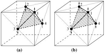
Figure 1: The ground state spin configuration of the FCC cell at the film surface: a) ordering of type I for $J_{s}<-0.5|J|$ b) ordering of type II for $J_{s}>-0.5|J|$.

III Monte Carlo Results

In this paragraph, we show the results obtained by MC simulations with the Hamiltonian (1) using the high-precision Wang-Landau flat histogram technique.WL1 Wang and Landau recently proposed a MC algorithm for classical statistical models. The algorithm uses a random walk in energy space in order to obtained an accurate estimate for the density of states $\rho(E)$ which is defined as the number of spin configurations for any given $E$. This method is based on the fact that a flat energy histogram $H(E)$ is produced if the probability for the transition to a state of energy $E$ is proportional to $\rho(E)^{-1}$. At the beginning of the simulation, the density of states (DOS) is set equal to one for all possible energies, $\rho(E)=1$. We begin a random walk in energy space $(E)$ by choosing a site randomly and flipping its spin with a probability proportional to the inverse of the momentary density of states. In general, if $E$ and $E^{\prime}$ are the energies before and after a spin is flipped, the transition probability from $E$ to $E^{\prime}$ is

$$p(E\rightarrow E^{\prime})=\min\left[\rho(E)/\rho(E^{\prime}),1\right].$$ (3)

Each time an energy level $E$ is visited, the DOS is modified by a modification factor $f>0$ whether the spin flipped or not, i.e. $\rho(E)\rightarrow\rho(E)f$. At the beginning of the random walk, the modification factor $f$ can be as large as $e^{1}\simeq 2.7182818$. A histogram $H(E)$ records how often a state of energy $E$ is visited. Each time the energy histogram satisfies a certain ”flatness” criterion, $f$ is reduced according to $f\rightarrow\sqrt{f}$ and $H(E)$ is reset to zero for all energies. The reduction process of the modification factor $f$ is repeated several times until a final value $f_{\mathrm{final}}$ which close enough to one. The histogram is considered as flat if

$$H(E)\geq x\%.\langle H(E)\rangle$$ (4)

for all energies, where $x\%$ is chosen between $70\%$ and $95\%$ and $\langle H(E)\rangle$ is the average histogram.

The thermodynamic quantitiesWL1 ; brown can be evaluated by

$$\langle E^{n}\rangle = \frac{1}{Z}\sum_{E}E^{n}\rho(E)\exp(-E/k_{B}T)$$

$$C_{v} = \frac{\langle E^{2}\rangle-\langle E\rangle^{2}}{k_{B}T^{2}}$$

$$\langle M^{n}\rangle = \frac{1}{Z}\sum_{E}M^{n}\rho(E)\exp(-E/k_{B}T)$$

$$\chi = \frac{\langle M^{2}\rangle-\langle M\rangle^{2}}{k_{B}T}$$

where $Z$ is the partition function defined by

$$Z=\sum_{E}\rho(E)\exp(-E/k_{B}T)$$ (5)

The canonical distribution at any temperature can be calculated simply by

$$P(E,T)=\frac{1}{Z}\rho(E)\exp(-E/k_{B}T)$$ (6)

In this work, we consider a energy range of interestSchulz ; Malakis $(E_{\min},E_{\max})$. We divide this energy range to $R$ subintervals, the minimum energy of each subinterval is $E^{i}_{\min}$ for $i=1,2,...,R$, and maximum of the subinterval $i$ is $E^{i}_{\max}=E^{i+1}_{\min}+2\Delta E$, where $\Delta E$ can be chosen large enough for a smooth boundary between two subintervals. The Wang-Landau algorithm is used to calculate the relative DOS of each subinterval $(E^{i}_{\min},E^{i}_{\max})$ with the modification factor $f_{\mathrm{final}}=\exp(10^{-9})$ and flatness criterion $x\%=95\%$. We reject the suggested spin flip and do not update $\rho(E)$ and the energy histogram $H(E)$ of the current energy level $E$ if the spin-flip trial would result in an energy outside the energy segment. The DOS of the whole range is obtained by joining the DOS of each subinterval $(E^{i}_{\min}+\Delta E,E^{i}_{\max}-\Delta E)$.

The film size used in our present work is $L\times L\times N_{z}$ where $L$ is the number of cells in $x$ and $y$ directions, while $N_{z}$ is that along the $z$ direction (film thickness). We use here $L=30,40,...,150$ and $N_{z}=$ 2, 4, 8, 12. Periodic boundary conditions are used in the $xy$ planes. Our computer program was parallelized and run on a rack of several dozens of 64-bit CPU. $|J|=1$ is taken as unit of energy in the following.

Before showing the results let us adopt the following notations. Sublattices 1 and 2 of the first FCC cell belongs to the surface layer, while sublattices 3 and 4 of the first cell belongs to the second layer [see Fig. 1(a)]. In our simulations, we used $N_{z}$ FCC cells, i.e. $2N_{z}$ atomic layers. We used the symmetry of the two film surfaces.

III.1 Crossover of the phase transition

As said earlier, the bulk FCC antiferromagnet with Ising spins shows a very strong first-order transition. This is seen in MC simulation even with a small lattice size as shown in Fig. 3.

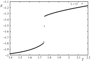
Figure 2: Bulk energy vs $T$ for $L=N_{z}=12$.

Figure 3: Bulk energy histogram for $L=N_{z}=12$ with periodic boundary conditions in all three directions (a) and without PBC in $z$ direction (b). The histogram was taken at the transition temperature $T_{c}$ indicated on the figure.

Our purpose here is to see whether the transition becomes second order when we decrease the film thickness. As it turns out, the transition remains of first order down to $N_{z}=4$ as seen by the double-peak energy histogram displayed in Fig. 4. Note that we do not need to go to larger $L$, the transition is clearly of first order already at $L=40$.

Figure 4: Energy histogram for $L=20,\ 30,\ 40$ with film thickness $N_{z}=4$ (8 atomic layers) at $T=1.8218,\ 1.8223,\ 1.8227$, respectively.

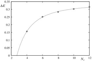
Figure 5: The latent heat $\Delta E$ as a function of thickness $N_{z}$.

In Fig. 5 we plot the latent heat $\Delta E$ as a function of thickness $N_{z}$. Data points are well fitted with the following formula

$$\Delta E=A-\frac{B}{N_{z}^{d-1}}\left[1+\frac{C}{N_{z}}\right],$$ (7)

where $d=3$ is the dimension, $A=0.3370,\ B=3.7068,\ C=-0.8817$. Note that the term $N_{z}^{d-1}$ corresponds to the surface separating two domains of ordered and disordered phases at the transition. The second term in the brackets corresponds to a size correction. As seen in Fig. 5, the latent heat vanishes at a thickness between 2 and 3. This is verified by our simulations for $N_{z}=2$. For $N_{z}=2$ we find a transition with all second-order features: no discontinuity in energy (no double-peak structure) even when we go up to $L=150$.

Before showing in the following the results of $N_{z}=2$, let us discuss on the crossover. In the case of a film with finite thickness studied here, it appears that the first-order character is lost for very small $N_{z}$. A possible cause for the loss of the first-order transition is from the role of the correlation in the film. If a transition is of first order in 3D, i. e. the correlation length is finite at the transition temperature, then in thin films the thickness effect may be important: if the thickness is larger than the correlation length at the transition, than the first-order transition should remain. On the other hand, if the thickness is smaller than that correlation length, the spins then feel an ”infinite” correlation length across the film thickness resulting in a second-order transition.

III.2 Film with 4 atomic layers ($N_{z}=2)$

Let us show in Fig. 6 and Fig. 7 the energy and the magnetizations of sublattices 1 and 3 of the first two cells with $L=120$ and $N_{z}=2$.

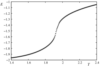
Figure 6: Energy versus temperature $T$ for $L=120$ with film thickness $N_{z}=2$.

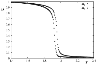
Figure 7: Sublattice magnetization for $L=120$ with film thickness $N_{z}=2$.

It is interesting to note that the surface layer has larger magnetization than that of the second layer. This is not the case for non frustrated films where the surface magnetization is always smaller than the interior ones because of the effects of low-lying energy surface-localized magnon modes.diep79 ; diep81 One explanation can be advanced: due to the lack of neighbors surface spins are less frustrated than the interior spins. As a consequence, the surface spins maintain their ordering up to a higher temperature.

Let us discuss on finite-size effects in the transitions observed in Figs. 8 and 9. This is an important question because it is known that some apparent transitions are artifacts of small system sizes.

To confirm further the observed transitions, we have made a study of finite-size effects on the layer susceptibilities by using the Wang-Landau technique described above.WL1

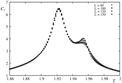
Figure 8: Specific heat are shown for various sizes $L$ as a function of temperature.

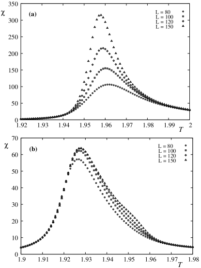
Figure 9: Susceptibilities of sublattice 1 (a) and 3 (b) are shown for various sizes $L$ as a function of temperature.

We observe that there are two peaks in the specific heat: The first peak at $T_{1}\simeq 1.927$, corresponding to the vanishing of the sublattice magnetization 3, does not depend on the lattice size while the second peak at $T_{2}\simeq 1.959$, corresponding to the vanishing of the sublattice magnetization 1, does depend on $L$. Both histograms taken at these temperatures and the near-by ones show a gaussian form indicating a non first-order transition [see Fig. 10].

Figure 10: Energy histograms for $L=120$ with film thickness $N_{z}=2$ at the two temperatures (indicated on the figure) corresponding to the peaks observed in the specific heat. See text for comment.

The fact that the peak at $T_{1}$ does not depend on $L$ suggests two scenarios:

i) the peak does not correspond to a real transition, since there exist systems where $C_{v}$ shows a peak but we know that there is no transition just as in the case of 1D Ising chain,

ii) the peak corresponds to a Kosterlitz-Thouless transition. To confirm this we need to check carefully several points such as the behavior of the correlation length etc. This is a formidable task which is not the scope of this work.

Whatever the scenario for the origin of the peak at $T_{1}$, we know that the interior layers are disordered between $T_{1}$ and $T_{2}$, while the two surface layers are still ordered. Thus, the transition of the surface layers occurs while the disordered interior spins act on them as dynamical random fields. Unlike the true 2D random-field Ising model which does not allow a transition at finite temperature,Imry the random fields acting on the surface layer are correlated. This explains why one has a finite-$T$ transition here. Note that this situation is known in some exactly solved models where partial disorder coexists with order at finite $T$.diep91honeyc ; diep91Kago ; Diep-Giacomini However, it is not obvious to foresee what is the universality class of the transition at $T_{2}$. The theoretical argument of Capehart and FisherFisher does not apply in the present situation because one does not have a single transition here, unlike the case of simple cubic ferromagnetic films studied before.Pham So, we wish to calculate the critical exponents associated with the transition at $T_{2}$.

The exponent $\nu$ can be obtained as follows. We calculate as a function of $T$ the magnetization derivative with respect to $\beta=(k_{B}T)^{-1}$: $V_{1}=\left<(\ln M)^{\prime}\right>=\left<E\right>-\left<ME\right>/\left<M\right>$ where $E$ is the system energy and $M$ the sublattice order parameter. We identify the maximum of $V_{1}$ for each size $L$. From the finite-size scaling we know that $V_{1}^{\max}$ is proportional to $L^{1/\nu}$.Ferrenberg3 We show in Fig. 11 the maximum of $V_{1}$ versus $\ln L$ for the first layer. We find $\nu=0.887\pm 0.009$. Now, using the scaling law $\chi^{\max}\propto L^{\gamma/\nu}$, we plot $\ln\chi^{\max}$ versus $\ln L$ in Fig. 12. The ratio of the critical exponents $\gamma/\nu$ is obtained by the slope of the straight line connecting the data points of each layer. From the value of $\nu$ we obtain $\gamma=1.542\pm 0.005$. These values do not correspond neither to 2D nor 3D Ising models ($\gamma_{2D}=1.75$, $\nu_{2D}=1$, $\gamma_{3D}=1.241$, $\nu_{3D}=0.63$). We note however that, if we think of the weak universality where only ratios of critical exponents are concerned,Suzuki then the ratios of these exponents $1/\nu=1.128$ and $\gamma/\nu=1.739$ are not far from the 2D ones which are 1 and 1.75, respectively.

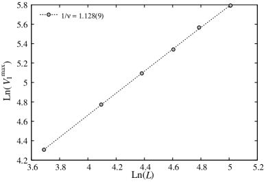
Figure 11: The maximum value of $V_{1}=\left<E\right>-\left<ME\right>/\left<M\right>$ versus $L$ in the $\ln-\ln$ scale. The slope of this straight line gives $1/\nu$.

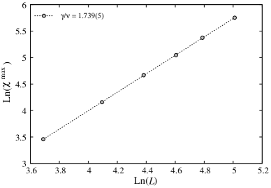
Figure 12: Maximum sublattice susceptibility $\chi^{\max}$ versus $L$ in the $\ln-\ln$ scale. The slope of this straight line gives $\gamma/\nu$.

IV Green’s Function Method

We consider here the same FCC system but with quantum Heisenberg spins. To compare the results with the Ising case, we add in the Hamiltonian an Ising-like anisotropy interaction term. In addition, this term avoids the absence of long-range order of isotropic non Ising spin model at finite temperature ($T$) when the film thickness is very small, i.e. quasi two-dimensional system.Mermin The Hamiltonian is given by

$$\mathcal{H}=-\sum_{\left<i,j\right>}J_{i,j}\mathbf{S}_{i}\cdot\mathbf{S}_{j}-\sum_{\left<i,j\right>}I_{i,j}S^{z}_{i}S^{z}_{j}$$ (8)

where $\mathbf{S}_{i}$ is the Heisenberg spin at the lattice site $i$, $\sum_{\left<i,j\right>}$ indicates the sum over the NN spin pairs $\mathbf{S}_{i}$ and $\mathbf{S}_{j}$. $J_{i,j}$ and $I_{i,j}$ are antiferromagnetic (negative). Note that in the laboratory coordinates, the up spins have $S^{z}\geq 0$ while the down spins have $S^{z}\leq 0$.

We can rewrite the Hamiltonian (8) in the relative local spin coordinates as

$$\mathcal{H} = -\sum_{<i,j>}J_{i,j}\Bigg{\{}\frac{1}{4}\left(\cos\theta_{ij}-1\right)\left(S^{+}_{i}S^{+}_{j}+S^{-}_{i}S^{-}_{j}\right)$$ (9)

$$+ \frac{1}{4}\left(\cos\theta_{ij}+1\right)\left(S^{+}_{i}S^{-}_{j}+S^{-}_{i}S^{+}_{j}\right)$$

$$+ \frac{1}{2}\sin\theta_{ij}\left(S^{+}_{i}+S^{-}_{i}\right)S^{z}_{j}-\frac{1}{2}\sin\theta_{ij}S^{z}_{i}\left(S^{+}_{j}+S^{-}_{j}\right)$$

$$+ \cos\theta_{ij}S^{z}_{i}S^{z}_{j}\Bigg{\}}-\sum_{<i,j>}I_{i,j}\cos\theta_{ij}S^{z}_{i}S^{z}_{j}$$

where $\theta_{ij}$ is the angle between two NN spins. Note that in the above expression, we have transformed all $S^{z}\geq 0$, the relative spin orientation of each spin pair is now expressed by $\theta_{ij}$. In a collinear spin configuration such as those shown in Fig. 1, $\cos\theta_{ij}=-1$ and $1$ for antiparallel and parallel pairs, respectively, while $\sin\theta_{ij}=0$. In non collinear structures, the calculation is more complicated. The general GF method for non collinear spin configuration has been proposed elsewhere.Rocco ; Santamaria In the present study, one has a collinear spin configuration shown in Fig. 1 because of the Ising-like anisotropy. We define two double-time GF by

$$G_{ij}(t,t^{\prime}) = \ll S^{+}_{i}(t);S^{-}_{j}(t^{\prime})\gg,$$ (10)

$$F_{mj}(t,t^{\prime}) = \ll S^{-}_{m}(t);S^{-}_{j}(t^{\prime})\gg.$$ (11)

where $i$ and $j$ belong to the up-spin sublattice, $m$ to the down-spin one. In the case of thin films, the reader is referred to Refs. diep79, ; diep81, ; Ngo07fccfilm, for a general formulation. We describe here only the main steps: we first write the equations of motion for $G_{ij}(t,t^{\prime})$ and $F_{mj}(t,t^{\prime})$ and we next neglect higher-order correlations by using the Tyablikov decoupling schemeTyablikov which is known to be valid for exchange terms,fro and then we introduce the following Fourier transforms in the $xy$ plane

$$G_{i,j}\left(t,t^{\prime}\right) = \frac{1}{\Delta}\int\int d\mathbf{k}_{xy}\frac{1}{2\pi}\int^{+\infty}_{-\infty}d\omega e^{-i\omega\left(t-t^{\prime}\right)}.$$ (12)

$$\hskip 19.91684ptg_{n,n^{\prime}}\left(\omega,\mathbf{k}_{xy}\right)e^{i\mathbf{k}_{xy}\cdot\left(\mathbf{R}_{i}-\mathbf{R}_{j}\right)},$$

$$F_{m,j}\left(t,t^{\prime}\right) = \frac{1}{\Delta}\int\int d\mathbf{k}_{xy}\frac{1}{2\pi}\int^{+\infty}_{-\infty}d\omega e^{-i\omega\left(t-t^{\prime}\right)}.$$ (13)

$$\hskip 19.91684ptf_{n,n^{\prime}}\left(\omega,\mathbf{k}_{xy}\right)e^{i\mathbf{k}_{xy}\cdot\left(\mathbf{R}_{m}-\mathbf{R}_{j}\right)},$$

where $\omega$ is the spin-wave frequency, $\mathbf{k}_{xy}$ denotes the wave-vector parallel to $xy$ planes, $\mathbf{R}_{i}$ is the position of the spin at the site $i$, $n$ and $n^{\prime}$ are respectively the indices of the layers where the sites $i$ (or $m$) and $j$ belong to. One has $n,n^{\prime}=1,2,...,2N_{z}$. The integral over $\mathbf{k}_{xy}$ is performed in the first Brillouin zone in the $xy$ reciprocal plane whose surface is $\Delta$. Finally, one obtains for all layers the following matrix equation

$$\mathbf{M}\left(\omega\right)\mathbf{g}=\mathbf{u},$$ (14)

Note that though $n$ runs from 1 to $2N_{z}$, the matrix $\mathbf{M}$ has the dimension of $4N_{z}\times 4N_{z}$ because for each $n$ there are two functions $g(n,n^{\prime})$ and $f(n,n^{\prime})$. In the above equation, $\mathbf{g}$ and $\mathbf{u}$ are the column matrices of dimension $4N_{z}$ which are defined as follows

$$\mathbf{g}=\left(\begin{array}[]{c}g_{1,n^{\prime}}\\ f_{1,n^{\prime}}\\ \vdots\\ g_{2N_{z},n^{\prime}}\\ f_{2N_{z},n^{\prime}}\\ \end{array}\right),\mathbf{u}=\left(\begin{array}[]{c}2\left<S^{z}_{1}\right>\delta_{1,n^{\prime}}\\ 0\\ \vdots\\ 2\left<S^{z}_{2N_{z}}\right>\delta_{2N_{z},n^{\prime}}\\ 0\\ \end{array}\right),$$ (15)

and

$$\mathbf{M}\left(\omega\right)=\left(\begin{array}[]{ccccccc}A^{+}_{1}&B_{1}&D^{+}_{1}&D^{-}_{1}&\cdots&\cdots&\cdots\\ -B_{1}&A^{-}_{1}&-D^{-}_{1}&-D^{+}_{1}&\cdots&\cdots&\cdots\\ C^{+}_{2}&C^{-}_{2}&A^{+}_{2}&B_{2}&D^{+}_{2}&D^{-}_{2}&\cdots\\ -C^{-}_{2}&-C^{+}_{2}&-B_{2}&A^{-}_{2}&-D^{-}_{2}&-D^{+}_{2}&\cdots\\ \cdots&\cdots&\cdots&\cdots&\cdots&\cdots&\cdots\\ \cdots&\cdots&\cdots&C^{+}_{N_{z}}&C^{-}_{N_{z}}&A^{+}_{N_{z}}&B_{N_{z}}\\ \cdots&\cdots&\cdots&-C^{-}_{N_{z}}&-C^{+}_{N_{z}}&-B_{N_{z}}&A^{-}_{N_{z}}\\ \end{array}\right)$$ (16)

where for the spin configuration of type I [Fig. 1 (a)] one has

$$A_{n}^{\pm} = \omega\pm\Bigg{[}2J_{n}\left<S^{z}_{n}\right>Z+8I_{n}\left<S^{z}_{n}\right>\Bigg{]}$$

$$B_{n} = -2J_{n}\left<S^{z}_{n}\right>\left(Z\gamma\right)$$ (17)

$$C_{n}^{+} = +4J_{n,n-1}\left<S^{z}_{n}\right>\cos\frac{k_{y}a}{2}$$ (18)

$$C_{n}^{-} = -4J_{n,n-1}\left<S^{z}_{n}\right>\cos\frac{k_{x}a}{2}$$ (19)

$$D_{n}^{+} = +4J_{n,n+1}\left<S^{z}_{n}\right>\cos\frac{k_{y}a}{2}$$ (20)

$$D_{n}^{-} = -4J_{n,n+1}\left<S^{z}_{n}\right>\cos\frac{k_{x}a}{2}$$ (21)

in which, $Z=4$ is the number of in-plane NN, and

$$\gamma=\frac{1}{Z}\left[4\cos\left(\frac{k_{x}a}{2}\right)\cos\left(\frac{k_{y}a}{2}\right)\right].$$

Here, for compactness we have used the following notations:

i) $J_{n}$ and $I_{n}$ are the in-plane interactions. In the present model $J_{n}$ is equal to $J=-1$. All $I_{n}$ are set to be $I(<0)$.

ii) $J_{n,n\pm 1}$ are the interactions between a spin in the $n$-th layer and its neighbor in the $(n\pm 1)$-th layer. Here, we take $J_{n,n\pm 1}=-1$. Of course, $J_{n,n-1}=0$ if $n=1$, $J_{n,n+1}=0$ if $n=2N_{z}$.

Now, solving det$(\mathbf{M})\equiv|\mathbf{M}|=0$, we obtain the spin-wave spectrum $\omega$ of the present system. For each $\mathbf{k}_{xy}$ there are $4N_{z}$ eigenvalues $\omega$, two by two with opposite signs because of the AF symmetry. The solution for the GF $g_{n,n}$ is given by

$$g_{n,n}=\frac{\left|\mathbf{M}\right|_{n}}{\left|\mathbf{M}\right|},$$ (22)

with $\left|\mathbf{M}\right|_{n}$ is the determinant made by replacing the $n$-th column of $\left|\mathbf{M}\right|$ by $\mathbf{u}$ in (15). Writing now

$$\left|\mathbf{M}\right|=\prod_{i}\left(\omega-\omega_{i}\left(\mathbf{k}_{xy}\right)\right),$$ (23)

one sees that $\omega_{i}\left(\mathbf{k}_{xy}\right),\ i=1,\cdots,\ 4N_{z}$, are poles of the GF $g_{n,n}$. Now, we can express $g_{n,n}$ as

$$g_{n,n}=\sum_{i}\frac{f_{n}\left(\omega_{i}\left(\mathbf{k}_{xy}\right)\right)}{\left(\omega-\omega_{i}\left(\mathbf{k}_{xy}\right)\right)},$$ (24)

where $f_{n}\left(\omega_{i}\left(\mathbf{k}_{xy}\right)\right)$ is

$$f_{n}\left(\omega_{i}\left(\mathbf{k}_{xy}\right)\right)=\frac{\left|\mathbf{M}\right|_{n}\left(\omega_{i}\left(\mathbf{k}_{xy}\right)\right)}{\prod_{j\neq i}\left(\omega_{j}\left(\mathbf{k}_{xy}\right)-\omega_{i}\left(\mathbf{k}_{xy}\right)\right)}.$$ (25)

Next, using the spectral theorem which relates the correlation function $\langle S^{-}_{i}S^{+}_{j}\rangle$ to the GF,zu one has

$$\left<S^{-}_{i}S^{+}_{j}\right> = \lim_{\varepsilon\rightarrow 0}\frac{1}{\Delta}\int\int d\mathbf{k}_{xy}\int^{+\infty}_{-\infty}\frac{i}{2\pi}\big{(}g_{n,n^{\prime}}\left(\omega+i\varepsilon\right)$$ (26)

$$- g_{n,n^{\prime}}\left(\omega-i\varepsilon\right)\big{)}\cdot\frac{d\omega}{e^{\beta\omega}-1}e^{i\mathbf{k}_{xy}\cdot\left(\mathbf{R}_{i}-\mathbf{R}_{j}\right)},$$

where $\epsilon$ is an infinitesimal positive constant and $\beta=1/k_{B}T$, $k_{B}$ being the Boltzmann constant.

Using the GF presented above, we can calculate self-consistently various physical quantities as functions of temperature $T$. Large values of Ising-like interaction $I$ will enhance the ordering. On the contrary, for $I\rightarrow 0$ the transition temperature will go to zero according to the Mermin-Wagner theorem.Mermin This is seen in the following. For numerical integretaion, we will use $80^{2}$ points in the first Brillouin zone.

Figure 13 shows the sublattice magnetizations of the first two layers for $N_{z}=2$ with $I=-0.25$ and $I=-0.01$ (upper and lower figures, respectively)). As seen, the surface sublattice magnetization is larger than the sublattice magnetization of the second layer for $N_{z}=2$ in qualitative agreement with the MC results shown in Fig. 7, in spite of the fact that due to a finite-size effect, there is a queue of the sublattice magnetization above the transition temperatures for MC results. Note that the AF coupling gives rise to a zero-point spin contraction at $T=0$ which is different for the surface spins and the second-layer spins.

We show in Fig. 14 the phase diagram in the space ($I,T)$ where $T_{1}$ and $T_{3}$ are transition temperatures of the surface sublattice 1 and the sublattice 3 of the second layer.

Figure 13: Magnetization of sublattices 1 (surface) and 3 (second layer) versus temperature for $N_{z}=2$ and $I=-0.25$ (upper) and $I=-0.01$ (lower).

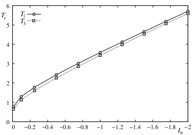
Figure 14: Phase diagram obtained by the GF method. $T_{1}$ and $T_{3}$ are transition temperatures of the sublattice 1 of the surface and of the sublattice 3 of the second layer. The transition temperatures should go to zero as $I\rightarrow 0$ (see text).

V Concluding Remarks

We have shown in this paper the crossover of the phase transition from first to second order in the frustrated Ising FCC AF film. This crossover occurs when the film thickness $N_{z}=2$ is smaller than a value between 2 and 4 FCC lattice cells. These results are obtained with the highly performing Wang-Landau flat histogram technique which allows to determine the first-order transition with efficiency.

For $N_{z}=2$, we found that in a range of temperature the surface spins stay ordered while interior spins are disordered. We interpret this as an effect of the frustration reduction: due to the lack of neighbors, the surface spins are less frustrated than the interior spins. As a consequence, interior spins are disordered at a lower temperature. This has been verified by the Green’s function calculation.

The second-order transition for $N_{z}=2$ is governed by the surface disordering and is characterized by critical exponents whose values are deviated from those of the 2D Ising universality class. We believe that this deviation results from the effect of the disordered interior spins which act as ”correlated” random fields on the surface spins. We do not know if the critical exponents found here belong to a new universality class or they are just ”effective critical exponents” which one could scale in some way or another to bring into the 2D Ising universality class. Anyway, these exponents seem to obey a weak universality. An answer to this question is desirable.

One of us (VTN) thanks the University of Cergy-Pontoise for a financial support and hospitality during the final stage of this work.

References

- (1) X. T. Pham Phu, V. Thanh Ngo and H. T. Diep, Surf. Science 603, 109 (2009).
- (2) T. W. Capehart and M. E. Fisher, Phys. Rev. B 13, 5021 (1976).
- (3) H. T. Diep, M. Debauche and H. Giacomini, Phys. Rev. B (rapid communication) 43, 8759 (1991).
- (4) M. Debauche, H. T. Diep, H. Giacomini and P. Azaria, Phys. Rev. B 44, 2369 (1991).
- (5) See reviews on theories and experiments given in Frustrated Spin Systems, ed. H. T. Diep, World Scientific (2005).
- (6) A. Zangwill, Physics at Surfaces, Cambridge University Press (1988).
- (7) Ultrathin Magnetic Structures, vol. I and II, J.A.C. Bland and B. Heinrich (editors), Springer-Verlag (1994).
- (8) H.W. Diehl, in Phase Transitions and Critical Phenomena, ed. by C. Domb, J.L. Lebowitz (Academic, London, 1986) vol. 10, H.W. Diehl, Int. J. Mod. Phys. B 11, 3503 (1997).
- (9) M. N. Baibich, J. M. Broto, A. Fert, F. Nguyen Van Dau, F. Petroff, P. Etienne, G. Creuzet, A. Friederich and J. Chazelas, Phys. Rev. Lett. 61, 2472 (1988).
- (10) P. Grunberg, R. Schreiber, Y. Pang, M. B. Brodsky and H. Sowers, Phys. Rev. Lett. 57, 2442 (1986); G. Binash, P. grunberg, F. Saurenbach and W. Zinn, Phys. Rev. B 39, 4828 (1989).
- (11) A. Barthélémy et al, J. Mag. Mag. Mater. 242-245, 68 (2002).
- (12) See review by E. Y. Tsymbal and D. G. Pettifor, Solid State Physics (Academic Press, San Diego), Vol. 56, pp. 113-237 (2001).
- (13) See V. Thanh Ngo, H. Viet Nguyen, H. T. Diep and V. Lien Nguyen, Phys. Rev. B. 69, 134429 (2004) and references on magnetic multilayers cited therein.
- (14) See V. Thanh Ngo and H. T. Diep, Phys. Rev. B. 75, 035412 (2007) and references on surface effects cited therein.
- (15) J. Villain, R. Bidaux, J. P. Carton, and R. Conte, J. Phys. (Paris) 41, 1263 (1980).
- (16) C. L. Henley, J. Appl. Phys. 61, 3962 (1987).
- (17) H. T. Diep and H. Kawamura, Phys. Rev. B 40, 7019 (1989).
- (18) C. Pinettes and H. T. Diep, J. Appl. Phys. 83, 6317 (1998).
- (19) J. L. Lebowitz and M. H. Kalos, Phys. Rev. B 21, 4027 (1980).
- (20) T. L. Polgreen, Phys. Rev. B 29, 1468 (1984).
- (21) D. F. Styer, Phys. Rev. B 32, 393 (1985).
- (22) J. Pommier, H. T. Diep, A. Ghazali and P. Lallemand, J. Appl. Phys. 63, 3036 (1988).
- (23) A. D. Beath and D. H. Ryan, Phys. Rev. B 73, 174416 (2006).
- (24) M. V. Gvozdikova and M. E. Zhitomirsky, JETP Lett. 81, 236 (2005).
- (25) H. T. Diep, Phys. Rev. B 45, 2863 (1992), and references therein.
- (26) V. Thanh Ngo and H. T. Diep, J. Appl. Phys. 103, 07C712 (2008).
- (27) V. Thanh Ngo and H. T. Diep, Phys. Rev. E, 78, 031119 (2008).
- (28) V. Thanh Ngo and H. T. Diep, J. Phys.: Condens. Matter (2007)
- (29) F. Wang and D. P. Landau, Phys. Rev. Lett. 86, 2050 (2001); Phys. Rev. E 64, 056101 (2001).
- (30) G. Brown and T.C. Schulhess, J. Appl. Phys. 97, 10E303 (2005).
- (31) B. J. Schulz, K. Binder, M. Müller, and D. P. Landau, Phys. Rev. E 67, 067102 (2003).
- (32) A. Malakis, S. S. Martinos, I. A. Hadjiagapiou, N. G. Fytas, and P. Kalozoumis, Phys. Rev. E 72, 066120 (2005).
- (33) Diep-The-Hung, J.C. S. Levy and O. Nagai, Phys. Stat. Solidi (b), 93, 351 (1979).
- (34) Diep-The-Hung, Phys. Stat. Solidi (b), 103, 809 (1981).
- (35) Yoseph Imry and Shang-Keng Ma, Phys. Rev. Lett. 35, 1399 (1975).
- (36) H. T. Diep and H. Giacomini, see chapter Frustration - Exactly Solved Frustrated Models in Ref. Diep2005, .
- (37) A. M. Ferrenberg and D. P. Landau, Phys. Rev. B 44, 5081 (1991).
- (38) Masuo Suzuki, Prog. Theor. Phys. 51, 1992 (1974).
- (39) N. D. Mermin and H. Wagner, Phys. Rev. Lett. 17, 1133 (1966).
- (40) See for example R. Quartu and H.T. Diep, Phys. Rev. B 55, 2975 (1997).
- (41) C. Santamaria, R. Quartu and H. T. Diep, J. Appl. Physics 84, 1953 (1998).
- (42) N. N. Bogolyubov and S. V. Tyablikov, Doklady Akad. Nauk S.S.S.R. 126, 53 (1959) [translation: Soviet Phys.-Doklady 4 604 (1959)].
- (43) P. Fröbrich, P. J. Jensen and P. J. Kuntz, Eur. Phys. J B 13, 477 (2000) and references therein.
- (44) D. N. Zubarev, Usp. Fiz. Nauk 187, 71 (1960)[translation: Soviet Phys.-Uspekhi 3 320 (1960)].