Accretion torques and motion of the hot spot on the accreting millisecond pulsar XTE J1807-294

Abstract

We present a coherent timing analysis of the 2003 outburst of the accreting millisecond pulsar XTE J1807$-$294 . We find an upper limit for the spin frequency derivative of $|\dot{\nu}|<5\times 10^{-14}\rm\,Hz/s$. The sinusoidal fractional amplitudes of the pulsations are the highest observed among the accreting millisecond pulsars and can reach values of up to 27$\%$ (2.5-30 keV). The pulse arrival time residuals of the fundamental follow a linear anti-correlation with the fractional amplitudes that suggests hot spot motion over the surface of the neutron star both in longitude and latitude. An anti-correlation between residuals and X-ray flux suggests an influence of accretion rate on pulse phase, and casts doubts on the use of standard timing techniques to measure spin frequencies and torques on the neutron star.

1. Introduction

An open problem in the field of accreting millisecond pulsar (AMXP) is how to devise a reliable method to measure spin and orbital parameters. Since the discovery of the first AMXP (Wijnands & van der Klis, 1998) considerable improvements have been made, leading to the measurement of accurate orbital and spin parameters for 9 of the 10 known AMXPs (see Wijnands 2004, Poutanen 2006, di Salvo et al. 2007 for a review and Patruno et al. 2009 for the last source discovered). Current methods (see e.g. Taylor 1992) are based on folding procedures to reconstruct the pulse profiles of the accreting neutron star and on direct measurement of the pulse phase variations due to orbital Doppler shift and spin changes (for example due to torques). The pulse phases are fitted using $\chi^{2}$ minimization techniques. However, a substantial complication sometimes arises due to the presence of a strong unmodeled noise component in the pulse phases that, when ignored, might affect the reliability of the method. Two possible strategies have been used in the literature to try and overcome this: (i) harmonic data selection (Burderi et al. 2006, Riggio et al. 2008, Chou et al. 2008, Papitto et al. 2007) and (ii) use of a minimum variance estimator (Boynton & Deeter 1985, Hartman et al. 2008). In the first case the pulse profiles are decomposed into their harmonic components: generally one sinusoid at the fundamental frequency (or first harmonic, $\nu$) and one at the second harmonic ($2\nu$) and are analyzed separately, measuring two independent sets of orbital and spin parameters. The harmonic with the weakest noise content is selected for the measurement of the spin and orbital parameters and the noisier one is discarded (see e.g., Burderi et al. 2006). Although this use of the most “stable” harmonic reduces the $\chi^{2}$, this selection throws away part of the information and in that sense is not optimal. The hypothesis behind the selection of the most stable harmonic is that, for unknown reasons, that harmonic better tracks the spin of the neutron star. Burderi et al. (2006) speculated that the second harmonic might be more stable because it arises from accretion onto both the polar caps and hence is insensitive to the flux ratio between poles.

In the second method, both harmonics are used and weighted to minimize the effect of phase noise (Boynton & Deeter 1985, Hartman et al. 2008). However, also in this second situation in practice data selection is performed. If the phases of both harmonics change differently, the possibility of defining pulse arrival times breaks down and the data where this happens have to be excluded from the analysis (Hartman et al., 2008).
Because both methods employ different data selections, different results are obtained when analyzing the same source. For example in the case of SAX J1808.4–3658, the pulse frequency derivative $\dot{\nu}$, measured from only the second harmonic was $4.4\times 10^{-13}\rm\,Hz\,s^{-1}$ for the first 14 days of the 2002 outburst and $-7.6\times 10^{-14}\rm\,Hz\,s^{-1}$ for the rest of the outburst (Burderi et al., 2006). In Hartman et al. (2008) we considered the same source and gave an upper limit of $|\dot{\nu}|<2.5\times 10^{-14}\rm\,Hz\,s^{-1}$ for all the four outbursts for which high resolution timing data was available. The reason for this discrepancy is that while Burderi et al. (2006) used only the information carried by the second harmonic and rejected the results of the fundamental frequency, we used both harmonics but excluded the initial data where the phase variations where stronger and discrepant between harmonics (Hartman et al., 2008). So these differences arise as a consequence of different data selections. In this paper we try to better characterize the timing noise such as observed in AMXPs focusing on a source where the noise is strong: XTE J1807-294 (J1807 from now on) which has been in outburst for $\approx 120$ days in 2003 (Markwardt et al., 2003).

2. Data reduction and reconstruction of the pulse profiles

We reduced all the pointed observations from the RXTE satellite taken with the Proportional Counter Array (PCA, Jahoda et al. 2006) that cover the 2003 outburst of J1807. The PCA instrument provides an array of five proportional counter units (PCUs) with a collecting area of 1200 $\rm\,cm^{2}$ per unit operating in the 2-60 keV range and a field of view with a FWHM of $\sim 1^{\circ}$.

We constructed the X-ray lightcurve using the counts in PCA Absolute channels 5-67 ($\approx 2.5-29$ keV).

We constructed our pulse profiles by folding 512 s long chunks of lightcurve in profiles of $N=32$ bins, with the ephemeris of Riggio et al. (2008). In this folding process we used the TEMPO pulsar timing program to generate a series of polynomial expansions of the ephemeris that predict the barycentered phase of each photon detected. The total number of photons detected in a single profile bin is $x_{j}\pm\sqrt{x_{j}}$, with the error calculated from counting statistics and $j=1,...,N$. Since the pulse profile shape changes throughout the outburst, it is not possible to base the analysis on a stable template profile. Therefore we decided to analyze the pulse profile harmonic components separately.

To calculate the pulse fractional amplitudes and phases we decomposed each profile as:

$$x_{j}=b_{0}+\displaystyle\sum_{k}b_{k}\rm\,cos\left\{\it 2\pi\left[\frac{k(j-0.5)}{N}-\phi_{k}\right]\right\}$$ (1)

by using standard $\chi^{2}$ minimization techniques. The term $b_{k}$ is the amplitude of the sinusoid representing the $k-$th harmonic, and $b_{0}$ is the unpulsed flux component. We choose the first peak of each sinusoid in the profile as the fiducial point for each harmonic. Defining the $k$-th harmonic frequency to be $k\cdot\nu$, the unique pulse phases $\phi_{k}$ of each harmonic range from 0 to 1. The i–th pulse time of arrival (TOA) of the k–th harmonic is then defined as: $t_{k,i}=\frac{\phi_{k}}{k\cdot\nu}+\Delta t_{i}$. Here $\Delta t_{i}$ is the time of the middle of the i-th folded chunk. With these definitions, a positive time shift is equivalent to a lagging pulse TOA, while a negative shift corresponds to a preceding pulse TOA. This is the convention that will be used later to define pulse phase residuals.

The fractional sinusoidal amplitude of the i-th pulse profile and the k-th harmonic is calculated as:

$$R_{i,k}=\frac{N\times b_{k}}{N_{ph,i}-B_{i}}$$ (2)

where $\rm N_{\it ph,i}$ and $\rm B_{\it i}$ are the total number of photons and the background counts (calculated with the FTOOL pcabackest) in the i-th pulse profile. The error on the fractional amplitude $R_{i,k}$ is calculated propagating the errors on $b_{k}$ and $N_{\it ph,i}$. The error on $B_{i}$ is negligible with respect to the other errors and will not be considered further.

We define a pulse profile harmonic to be significant if the ratio between the amplitude $b_{k}$ and its statistical error $\sigma_{b_{k}}$ is larger than 3.3 when using a folding time of 512 s. The choice of 3.3 guarantees that the number of false detections expected when considering the global number of pulse profiles ($\approx 850$), is less than one. The length of the folding time was then changed to 300 and $3000$ s to probe different timescales (see §3), and the significance threshold rescaled to 3.5 and 3$\sigma$ respectively, according to the new number of pulse profiles.

After obtaining our set of TOAs for all the significant harmonics we chose to describe the phase $\phi$ of the k-th harmonic (we omit the k index from now on) at the barycentric reference frame, as a combination of six terms:

$$\phi\left(t\right)=\phi_{L}\left(t\right)+\phi_{Q}\left(t\right)+\phi_{O}\left(t\right)+\phi_{M}\left(t\right)$$

$$+\phi_{A}\left(t\right)+\phi_{N}\left(t\right)$$ (3)

where $\phi_{L}\left(t\right)$ is a linear function of the time ($\phi_{L}\left(t\right)=\phi_{0}+\nu\,t$, with $\phi_{0}$ an initial reference phase), $\phi_{Q}\left(t\right)$ is a parabolic function of time ($\phi_{Q}\left(t\right)=\frac{1}{2}\dot{\nu}t^{2}$), and $\phi_{O}\left(t\right)$ is the keplerian orbital modulation component. The term $\phi_{M}\left(t\right)$ is the measurement error component, and is given by a set of independent values and is normally distributed with an amplitude that can be predicted by propagating the Poisson uncertainties due to counting statistics. The term $\phi_{A}\left(t\right)$ is the astrometric uncertainty position error, and the last term, $\phi_{N}\left(t\right)$, is the so-called timing noise component that defines all the phase variations that remain. The timing noise includes, but is not limited to, any phase residual that can be described as red noise and possible extra white noise in addition to that described by the measurement error component $\phi_{M}\left(t\right)$.

One of the key points when dealing with timing noise is how to distinguish a true spin frequency change of the neutron star from an effect that mimics it. In general, $\phi_{Q}$ and $\phi_{N}$ can both be due to torques, both not be due to torques, or one can, while the other is not. In the first case the torque is not constant and has a fluctuating component. In the second case there is a process different from a torque affecting the pulse phases. In the third case, if $\phi_{Q}$ is due to a torque, it is constant, while if $\phi_{N}$ is due to a torque then the torque is not constant.

In the presence of timing noise ($\phi_{N}$) the formal parameter errors estimated using standard $\chi^{2}$ minimization techniques are not realistic estimates of the true uncertainties, as the hypothesis behind the $\chi^{2}$ minimization technique is that the source of noise is white and its amplitude can be predicted from counting statistics. In the presence of an additional source of noise, such as the timing noise, the apparently significant measurement of a parameter can simply reflect the non realistic estimation of the parameter errors. To solve this, we adopted the technique we already employed in Hartman et al. (2008), who used Monte Carlo (MC) simulations of the timing residuals to account for the effect of timing noise on the parameter errors. The technique uses the power density spectrum of the best-fit timing residuals of a $\dot{\nu}$ model, as output by TEMPO. Then thousands of fake power density spectra are produced, with Fourier amplitudes identical to the original spectrum and with random uncorrelated Fourier phases. The Fourier frequencies are then transformed back to the time domain into fake residuals, and thousands of $\nu$ and $\dot{\nu}$ values are measured to create a Gaussian distribution of spin frequencies and spin frequency derivatives. The standard deviations of these distributions are the statistical uncertainties on the spin frequency and derivative. For a detailed explanation of the method we refer to Hartman et al. (2008).

3. Results

3.1. Measurement of the spin frequency and its derivative in the presence of timing noise

We fitted the phases of each harmonic with a circular keplerian model ($\phi_{O}$) plus a linear term ($\phi_{L}$) and a quadratic term ($\phi_{Q}$). All the residual phase variation we observe after removing these three terms is treated as noise ($\phi_{M}$ and $\phi_{N}$). The $\nu$ and $\dot{\nu}$ measured for each of the two harmonics is given in Tables 1 and 2, respectively. The errors on the pulse frequency and its derivative are calculated performing $10^{4}$ MC simulations as described in § 2. At long periods (days), red noise dominates the power spectrum, while at short periods (hours), the uncorrelated Poisson noise dominates. The red noise power spectrum is not very steep, and has a power law dependence $P(\nu)\propto\nu^{\alpha}$ with $\alpha\approx-0.5$.

The source position we used comes from Chandra observations whose $68\%$ confidence level error circle is $0^{\prime\prime}.4$ in radius. The astrometric uncertainty introduced in this way on the frequency and frequency derivative is $3\times 10^{-8}\rm\,Hz$ and $0.7\times 10^{-14}\rm\,Hz\,s^{-1}$, respectively (calculated with eqs. A1 and A2 from Hartman et al. (2008), which added in quadrature to the MC statistical errors gives the final errors reported in Tables 1 and 2. The final pulse frequency derivative significances for the fundamental and the second harmonic are $\approx 2.7\sigma$ and $\approx 1.5\sigma$, respectively.

We note that the significance of the frequency derivative for the fundamental increases above the 3 sigma level when the statistical errors are calculated with standard $\chi^{2}$ minimization techniques, consistently with Riggio et al. (2008). These errors calculated with $\Delta\chi^{2}=1.0$ are $2\times 10^{-16}\rm\,Hz\,s^{-1}$ and $1.6\times 10^{-15}\rm\,Hz\,s^{-1}$ for the fundamental and second harmonic respectively. So, a significant $\dot{\nu}$ is present which is, however, consistent with being part of the (red) timing noise.

The timing residuals obtained after removing a $\dot{\nu}=0$ model are plotted in Figure 1 for both the harmonics (see Tables 1 & 2 for the pulse frequencies used in the fits). Our orbital solution is consistent for the two harmonics and with the orbital parameters published in Riggio et al. (2008). For the fundamental we find:

• orbital period: 2404.4163(3) s

• projected semi-major axis: 4.830(3) lt-ms

• time of ascending node: MJD 52720.675601(3)

where the quoted errors are calculated with the $\chi^{2}$ minimization technique and correspond to $\Delta\chi^{2}=1$. Since the pulse phase residuals are approximately white and consistent with the expected Poissonian uncertainty, on timescales equal to and shorter than the orbital period, the orbital parameter errors are a good approximation of the true uncertainties.

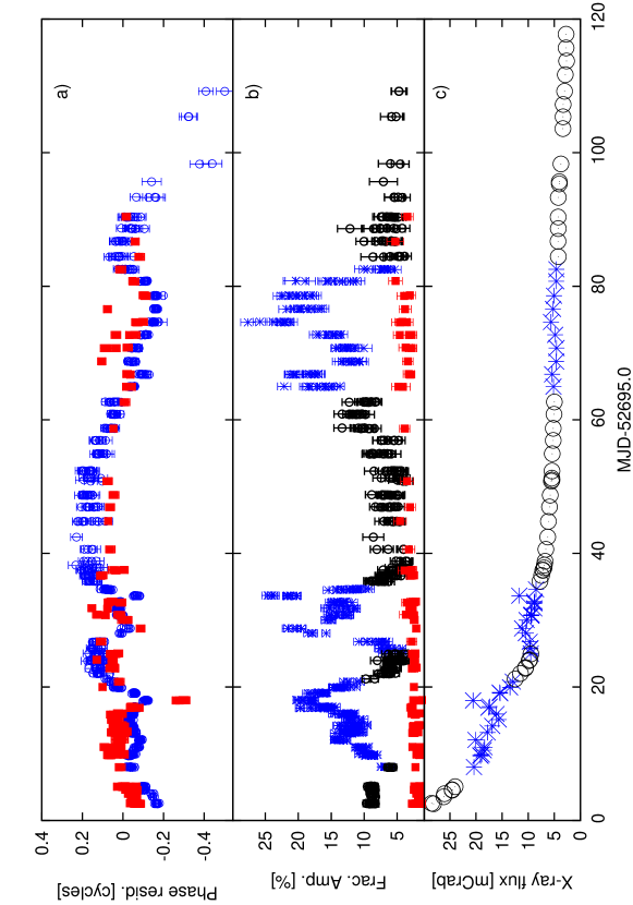
Figure 1.— a): Timing residuals for a constant spin frequency and a circular keplerian orbit. The fundamental (blue circles) and the second harmonic (red squares) phases were measured using an integration time of $512$ s per pulse profile.
b): Sinusoidal fractional amplitude of the fundamental (blue asterisks: flaring; black circles: non-flaring) and second harmonic (red squares) during the whole outburst. During the flares, the fundamental sinusoidal fractional amplitude grows up to $\approx 27\%$, which is the highest value ever observed for an AMXP.
c): XTE J1807$-$294 lightcurve of the 2003 outburst. The count rate was normalized to the Crab (Kuulkers et al., 1994) using the data nearest in time and in the same PCA gain epoch (e.g., van Straaten et al. 2003). The blue circles and the black asterisks identify the 4 non-flaring and the 3 flaring states, respectively, as defined in Chou et al. (2008).

Table 1Timing parameters for XTE J1807-294 (Fundamental)

Parameter	Fundamental	MC error	Astrometric error	Final error
Spin frequency $\nu$ (Hz)	190.62350702	$2\times 10^{-8}$Hz	$3\times 10^{-8}$Hz	$4\times 10^{-8}$Hz
Spin frequency derivative $\dot{\nu}\rm\,(10^{-14}Hz\,s^{-1})$	$2.7$	$0.7$	$0.7$	$1.0$
Reference Epoch (MJD)	52720.0

Table 2Timing parameters for XTE J1807-294 (second harmonic)

Parameter	second harmonic	MC error	Astrometric error	Final error
Spin frequency $\nu$ (Hz)	190.62350706	$3\times 10^{-8}$Hz	$3\times 10^{-8}$Hz	$4\times 10^{-8}$Hz
Spin frequency derivative $\dot{\nu}\rm\,(10^{-14}Hz\,s^{-1})$	1.6	$0.8$	$0.7$	$1.1$
Reference Epoch (MJD)	52720.0

3.2. Relation between timing residuals and X-ray flux

In this section we analyze the relation between the pulse arrival time residuals relative to a constant pulse frequency ($\dot{\nu}=0$) model and X-ray flux. Riggio et al. (2008) found that the residuals of the fundamental show a strong correlation with the X-ray flux, while the second harmonic shows only a marginal correlation. Since large pulse phase shifts are often observed (in both harmonics) in coincidence with the flaring states, we investigate the possibility that at least part of the observed timing noise is correlated with the presence of X-ray flux variations.

In this section we show that both the harmonics are consistent with being correlated with X-ray flux. First we focus on the entire data set, then we split the data in intervals choosing the same 7 chunks as Chou et al. (2008); see Figure 1c), distinguishing non-flaring states following the exponential flux decay of the overall outburst, and flaring states, comprising the six spikes in the lightcurve. In Figure 2 we plot the residuals vs. the count rate for both the fundamental and the second harmonic.

We applied a Spearman rank correlation test to the flux anti-correlation for each harmonic. We accept the null hypothesis (no correlation in the data set) if the probability $p>1\%$. If we do not make any data selection, the Spearman test shows no correlation in either harmonic. However, a clear split in the data is apparent at around 7 mCrab: below this threshold the residuals seem to follow a correlation with the flux, while above this threshold an anti-correlation is visible for both harmonics. The Spearman coefficients for the points above the threshold are $\rho=-0.8$ and $\rho=-0.65$ for the fundamental and the second harmonic respectively ($p<1\%$). A few outliers are visible in the plot, such as for example the four points of the second harmonic at about $\approx-0.3$ cycles. These points correspond to data taken during some of the flaring states. If we consider only the non-flaring states, the Spearman coefficients become $\rho=-0.9$ and $\rho=-0.76$ respectively ($p<1\%$).

The fact that we see a change from correlation to anti-correlation around $7$ mCrabs is due to the fact that at that flux level in the decay of the outburst the timing residuals reach the peak of the parabolic function that dominates the residuals (at MJD$\approx 52745$, see Figure 1). This is a consequence of the fitting procedure, which selects the constant reference pulse frequency that minimizes the $\chi^{2}$ of the timing residuals. As the observed pulse frequency is increasing, the reference frequency is too fast for the rising part of the residuals, and too slow for the decreasing part.

We have seen in § 3.1 that the measured pulse frequency increase is consistent with being part of a red noise process and that true neutron star spin variations may or may not be the cause. We can choose a higher reference pulse frequency than the one used to produce Figure 1a, and turn the correlation-anti-correlation dichotomy in the flux-residual diagram into only an anti-correlation, at the cost of increasing $\chi^{2}$ by a factor $\approx 10$. A $\nu$ higher by $10^{-7}\rm\,Hz$ makes the split in the data disappear and increases the degree of correlation between flux and timing residuals.

All the correlations and anti-correlations disappear or are strongly reduced for the timing residuals relative to the best-fit finite constant-$\dot{\nu}$ model.

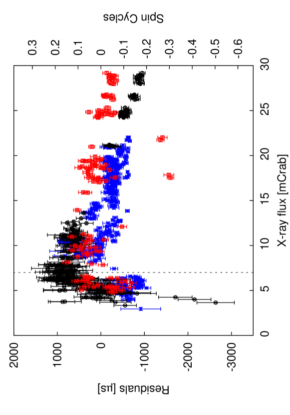
Figure 2.— Phase residuals vs. X-ray flux for the fundamental (blue asterisks for the flaring intervals and open black circles for the non-flaring intervals) and the second harmonic (red open squares) relative to a $\dot{\nu}=0$ model. Each pulse is a 512 s folded chunk of lightcurve. The dashed line at around 7 mCrab splits the diagram in two regions: in the left one the points follow a correlation, in the right one they follow an anti-correlation. The four points of the second harmonic that lay outside the relations correspond to the large jump observed during the second flare.

3.3. Pulse profiles

In this section we focus on the shape of the pulse profiles and their relation with other observables, such as the phase, the timing noise and the X-ray flux.

3.3.1 The fractional amplitude-residual diagram

We have seen in the previous section that for some data selections the X-ray flux correlates with the timing residuals relative to a $\dot{\nu}=0$ model, but not when a finite $\dot{\nu}$ is admitted. As already noticed by Zhang et al. (2006) and Chou et al. (2008), the fractional amplitude of the pulsations shows six spikes coincident with the six flares in the lightcurve. Therefore, a correlation might also exist between the fractional amplitude of the pulsations and the arrival time residuals. Using a $\dot{\nu}=0$ model, and again using a Spearman rank test, we found a correlation coefficient $\rho=-0.61$ ($p<1\%$) for the fundamental, while no significant correlation exists for the second harmonic. The second harmonic is also inconsistent with following the same correlation as the fundamental. Repeating the test for a $\dot{\nu}$ model we still find no correlations for the second harmonic, but the anti-correlation found for the fundamental becomes stronger ($\rho=-0.80$, $p<1\%$). In Figure 3 we show the fractional amplitude vs. residual diagram (relative to a $\dot{\nu}$ model). The anti-correlation is evident. It is interesting that the small number of points (circled in the figure) that are outliers all belong to the first 2.5 days of the outburst.

We then analyzed the flaring and non-flaring states separately. The non-flaring state shows a weak anti-correlation with a $\dot{\nu}=0$ model ($\rho=-0.43$, $p<1\%$) which becomes slightly stronger with a $\dot{\nu}$ model ($\rho=-0.51$, $p<1\%$) The flaring state shows an anti-correlation relative to a $\dot{\nu}=0$ model ($\rho=-0.58$, $p<1\%$) that becomes much stronger for a $\dot{\nu}$ model ($\rho=-0.81$, $p<1\%$).

We found no energy dependence in this fractional amplitude-timing residual anti-correlation (amplitude anti-correlation from now on) when we repeated the analysis in 6 different energy bands from 2.5 to 30 keV. The same is true for the second harmonic: no correlation was found in any energy band.

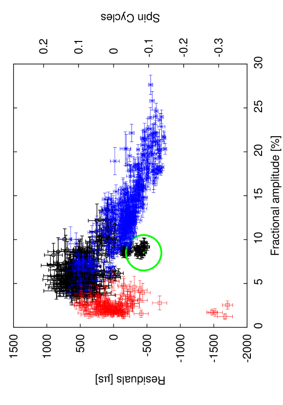
Figure 3.— Timing residuals vs. fractional amplitude diagram. The blue asterisks refer to the flaring states, while the black circles are the non-flaring states, both referring to the fundamental frequency. The second harmonic is plotted as red open squares. Each pulse was built using 512 s of integration time. The residuals are relative to a finite $\dot{\nu}$ model. The green circled outliers of the anti-correlation for the fundamental, all belong to the first 2.5 days of the observations. The second harmonic amplitude is uncorrelated to timing residuals.

3.3.2 The X-ray flux and the fractional amplitude

In our previous paper (Hartman et al., 2008), we found an anti-correlation between the fractional amplitude of the second harmonic and the X-ray flux in SAX J1808.4$-$3658. We also noted that the fractional amplitude of the fundamental behaved unpredictably. Something similar applies to J1807, where no correlation is found for the fundamental while a strong anti-correlation exists between the observed count rate and the fractional amplitude of the second harmonic ($\rho=-0.79$, $p<1\%$, see Figure 4). The behavior of the fundamental is inconsistent with this relation. By analogy with Hartman et al. (2008) we fitted a simple power-law model ($R_{2}\propto f^{\gamma}_{x}$, where $f_{x}$ is the X-ray flux) to the data, which gives a power law index $\gamma=-0.41\pm 0.04$ with a $\chi^{2}$/dof of 90.2/117. Interestingly, the power law index we found for SAX J1808.4$-$3658 (Hartman et al., 2008) was in agreement with this. So, a difference in behavior exists between the fractional amplitude of the fundamental frequency and of the second harmonic. They respond differently to both the flux and the arrival time residuals.

Figure 4.— The fractional amplitude of the second harmonic is anti-correlated with the flux and scales with a power law of index $\gamma=-0.41\pm 0.04$, close to the power law index found in a similar relation for SAX J1808.4$-$3658.

3.3.3 Fractional amplitude

We focus now on the energy dependence of the pulse profiles. We consider again all the data available and the subgroups of flaring and non-flaring states. Chou et al. (2008) already reported on the energy dependence of the fundamental frequency during the non flaring state. Here we explore also the flaring state and the energy dependence of the second harmonic. Looking at Figure 5 two interesting features are immediately apparent:
1. the fractional amplitude energy dependence is the same for both harmonics and regardless of the state of the source (flaring, non-flaring), up to a constant factor
2. the fractional amplitude of the fundamental increases by a factor of $\approx 1.8$ during the flaring state with respect to the non-flaring state, while it remains approximately constant for the second harmonic.
Another important property of the pulses is the time dependence of the fractional amplitude. In the middle panel of Figure1 we plot the fractional amplitude of the pulsations in the $2.5-30$ keV band. As can be seen, during the last of the six flaring states the fractional amplitude of the fundamental increases up to $\approx 27\%$, which is the highest ever observed for an AMXP. Selecting a narrower band between 2.5 and 10 keV the maximum fractional amplitude does not appreciably change. During the non-flaring stage the fractional amplitude decreases smoothly from $\approx 9\%$ down to $\approx 4\%$. The second harmonic amplitude on the contrary increases from $\approx 2\%$ up to $\approx 5\%$.

3.3.4 Harmonic content

We decomposed each pulse profile in its harmonic components to look for the presence of higher harmonics. While the detection of the second harmonic is quite common among the AXMPs, higher harmonics have never been detected, with the exception of a possible third harmonic in SAX J1808.4$-$3658 (Hartman et al., 2008). In J1807 we detected a third harmonic at better than 3$\sigma$, in several different stages of the outburst, with a maximum fractional amplitude of $\approx 1.5\%$ at MJD around 52560. To increase the S/N, we folded chunks of data of length $3000$ s. The number of $>3\sigma$ detections of the third harmonic was of 11 out of 163 chunks searched. We searched the same chunks for a fourth harmonic, and found 5-10 significant detections above 3$\sigma$ in the whole outburst, depending on the binning. When detected, the fourth harmonic has a fractional amplitude $0.5-2.0\%$.

There were no observations where we detected all 4 harmonics at the same time. During the second and third flares, we found a second and fourth but not a third harmonic, during the first two flares we found a second and third but not a fourth harmonic.

For the third and fourth harmonics we count respectively 8 and 5 detections during the flaring states and 3 and 2 detections in the non-flaring states.

The fractional amplitude of the third harmonic also decreases with the flux, although the slope of the power law is much smaller ($\gamma=-0.017\pm 0.004$). The fourth harmonic has no significant flux dependence, but its power law slope is also consistent with the $\gamma$ obtained for the third harmonic.

Of course this result has to be taken with caution, since we are suffering from low number statistics with only $\approx 20$ detections of the third and fourth harmonic altogether.

Figure 5.— Energy dependence of the pulse fractional amplitudes. The squares and the triangles refer to the flaring and non-flaring states respectively. The circles comprise the whole outburst. The bottom curves, overlapped in the plot, are the fractional amplitudes of the second harmonic which remains stable in both states. The pulses of the fundamental in the flaring states have a fractional amplitude which is about 1.8 times larger than during the non-flaring states. Up to a constant factor, the fractional amplitude has the same energy dependence for both harmonics and for both flaring and non-flaring states.

3.4. Short-term $\dot{\nu}$ measurements

Using the fundamental frequency, we measured short-term pulse frequency derivatives using the seven sub groups of data as defined in §3.2. These measurements are useful to investigate the time dependence of the pulse frequency derivative with time. This test is possible in J1807 because of its very long outburst duration (more than 120 days, of which $\approx 106$ days with detectable pulsations).

The $\dot{\nu}$ values and their uncertainties were first calculated with standard $\chi^{2}$ minimization techniques. All measured $\dot{\nu}$ values during the non-flaring states had a positive sign, whereas a negative sign was measured for all three flaring states. The measured $\dot{\nu}$ values are shown in Figure 6. There is no clear trend, and most importantly no correlation between $\dot{\nu}$ and the average X-ray flux in either the flaring and the non-flaring states. This test cannot be performed on the second harmonic, since the smaller number of detections prevents a meaningful analysis of data subsets for this purpose.

We then calculated the statistical uncertainties on the $\dot{\nu}$ for each sub group of data by using the MC method as explained in § 3.1. All the $\dot{\nu}$ values were consistent with being part of the same red noise process, consistently with what was calculated for the long term $\dot{\nu}$ value of § 3.1.

Figure 6.— Frequency derivative ($\dot{\nu}$) evolution. The non flaring states (open circles) all have positive $\dot{\nu}$, that however does not follow a power-law decrease as expected from the accretion theory. The flaring states (asterisks) all have a negative value, corresponding to spin down.

4. Discussion

We have analyzed the outburst of XTE J1807-294 and we have calculated statistical errors by means of MC simulations as we previously did for SAX J1808.4-3658 (Hartman et al., 2008). We found that with our statistical treatment of the red noise observed in the timing residuals of both the fundamental and the second harmonic, the significance of the spin up is reduced below 3$\sigma$ for both the fundamental and the second harmonic.

The fact that the spin frequency derivative is not significant does not mean that there is not a component in the residuals that can be fitted with a parabola. It just means that the parabola is consistent with having the same origin as the power at other low frequencies: both the parabola and the remaining fluctuations are consistent with being part of the realization of the same red noise process in the timing residuals. It is a separate issue whether or not this process is due to true spin changes and torques on the neutron star.

Our observed parabola in the timing residuals combined with the stochastic and astrometric uncertainty implies that any spin frequency derivative has a magnitude smaller than $|\dot{\nu}|{\thinspace\hbox to0.0pt{\raise 2.15277pt\hbox{$\scriptstyle{<}$}\hss}{\lower 1.29167pt\hbox{$\scriptstyle{\sim}$}}\thinspace}5\times 10^{-14}\rm\,Hz\,s^{-1}$ at the $95\%$ confidence level.

Evidence against the spin-up interpretation of the phases comes from the lack of any correlation between the observed X-ray flux and the measured $\dot{\nu}$ (see § 3.4). If standard accretion torque theory applies, then the magnetospheric radius ($r_{m}$) should decrease as the mass accretion rate $\dot{M}$ increases, following a power-law $r_{m}\propto\dot{M}^{-\alpha}$ when $r_{m}<r_{co}$, with $\alpha=2/7$ in the simplest case, where $r_{co}$ is the corotation radius. This implies that also the instantaneous $\dot{\nu}$ has a power-law dependence on the mass accretion rate, and (when $r_{m}<r_{co}$) it is:

$$\dot{\nu} = \frac{\dot{M}\sqrt{GMr_{m}}}{2\pi I}\simeq 1.6\times 10^{-13}\rm\,Hz\,s^{-1}$$ (4)

$$\times \left(\frac{\dot{M}}{10^{-10}M_{\odot}\rm\,yr^{-1}}\right)\left(\frac{\nu}{\rm\,Hz}\right)^{-1/3}\left(\frac{r_{m}}{r_{co}}\right)^{1/2}$$

see Bildsten et al. (1997). Here $\dot{M}$ is the average mass accretion rate, M the neutron star mass and $I$ the neutron star moment of inertia. We have observed no such a correlation between the flux and the instantaneous pulse frequency derivative, neither in the flaring nor in the non-flaring states. One possible explanation is that the X-ray flux is not a good tracer of the mass accretion rate. If it is, standard accretion theory does not apply and the most logical conclusion is that the observed timing residuals are not due to torques.

The possibility that the X-ray flux is not a good tracer of the mass accretion rate is a long standing issue in the X-ray binary pulsar field and has no simple solution. If the X-ray flux is completely unrelated to the mass accretion rate, then no conclusions can be drawn on the effect of the accretion on the pulse phase.

By using eq. (4) we can calculate the spin frequency derivative expected for J1807 from standard accretion theory, assuming a distance of 8 kpc and converting the average X-ray luminosity into an average mass transfer rate through $L_{x}\approx\eta c^{2}\dot{M}$. We assume an efficiency $\eta=0.1$ for the conversion of gravitational potential energy into radiation. In this way we obtain an average mass accretion rate $\dot{M}\approx 3\times 10^{-11}M_{\odot}\rm\,yr^{-1}$ (averaging over the outburst). Assuming $r_{m}\approx r_{co}$ we have an expected $\dot{\nu}\approx 10^{-14}\rm\,Hz\,s^{-1}$, which is below our calculated upper limit of $5\times 10^{-14}\rm\,Hz\,s^{-1}$. However, the short term $\dot{\nu}$ values calculated in §3.4 exceed the theory value by 1–2 orders of magnitude and therefore are very unlikely due to accretion torques.

The possibility that we are not observing the effect of a torque on the neutron star is also suggested by the fact that looking at the shape of the lightcurve one can immediately infer the sign of the measured pulse frequency derivative in the timing residuals. This is a consequence of the flux anti-correlation. If the lightcurve is concave, then the average $\dot{\nu}$ is positive, while if the lightcurve has a convex shape the average $\dot{\nu}$ will be negative. This explains why $\dot{\nu}>0$ in the non-flaring states and $\dot{\nu}<0$ in the flaring states. It suggests a direct influence of the accretion rate on phase, which could be effectuated through the hot spot position on the neutron star surface. Extending this interpretation to the average $\dot{\nu}$ over the entire outburst, we also favor the interpretation of a moving hot spot for that long term trend, discarding the hypothesis of a torque to explain the parabola observed in the pulse phase residuals.

Chou et al. (2008) also suggested that the lagging arrival times observed during the flaring states cannot be explained with a torque model, since they correspond to a sudden change from a spin up to a spin down. These authors also suggested that motion of the hot spot can be responsible for both the phase shifts and the increase of the fractional amplitude during the flaring states. Chou et al. (2008) assumed a fixed position of the hot spot during the non-flaring states. However, it is unlikely that the hot spot is fixed on the surface during the non-flaring state, as we have shown (see § 3.4) that the magnitude of the short-term $\dot{\nu}$ is too large to be compatible with standard accretion theory.

Ibragimov & Poutanen (2009) recently proposed a receding disk as a possible explanation for the timing noise and pulse profile variability observed in the 2002 outburst of SAX J1808.4-3658. In this model the antipodal spot can be observed when the inner accretion disk moves sufficiently far from the neutron star surface as a consequence of decreasing flux. We observed a strong overtone and pulse phase drifts since the early stages of the outburst, when the disk should be closest to the neutron star. Therefore it is not clear whether our observations can be explained by this model or not, and further investigations of the problem are required.

Two hot spots with different and variable intensities can produce a phase shift and a changing pulsed amplitude, even if the location of both hot spots is fixed on the neutron star surface (Burderi, 2008). This possibility needs also further investigation since a self-consistent model has not yet been presented.

We observed (1) a relation between flux and time of arrivals for both the flaring and non-flaring state (§ 3.2). This relation was consistent with being the same for the two states. We also observed (2) an anti-correlation between pulse fractional amplitudes and time of arrivals during the flaring state. Finally, (3) this amplitude anti-correlation became stronger when using a long term $\dot{\nu}$. The amplitude anti-correlation was weak in the non-flaring state, regardless of the $\dot{\nu}$. In the context of a hot spot motion model for the time of arrival variations, these findings constrain the kinematics of this motion.

Lamb et al. (2008) demonstrated that variations in the pulse fractional amplitudes should be anti-correlated with their time of arrival if the hot spot is close to the neutron star spin axis and the hot spot wanders by a small amount in latitude.

Lamb et al. (2008) showed that even a small displacement in longitude of the emitting region, when close to the spin axis, produces a large phase change, but no amplitude variation. A motion in latitude produces both phase and amplitude changes due to the hot spot velocity variation affecting Doppler boosting and aberration. An anti-correlation between the pulse arrival times and the pulse amplitudes would be an indicator of the above. Combining this with our observational findings 1-3 above we conclude within the moving hot spot model for the phase variation that:

1. the hot spot moves with flux in both flaring and non-flaring state, since the relation between flux and arrival times is observed in both cases and is consistent with being the same,

2. the amplitude anti-correlation in the flaring state implies an hot spot moving in latitude. The hot spot cannot move mainly in latitute during the non-flaring state since a weak amplitude anti-correlation is observed and the fractional amplitude changes by only a factor $\approx 2$ in $106$ days.

3. The long term $\dot{\nu}$ must be related with a motion in longitude since during the flaring state the amplitude anti-correlation becomes much stronger when a $\dot{\nu}$ model is used to fit the time of arrivals. This is also compatible with the non-flaring state, since the amplitude anti-correlation remains weak with or without a $\dot{\nu}$.

4. Finally a motion in longitude during the flaring state or in latitude during the non-flaring state is possible, but it has to be small enough to preserve the observed flux and amplitude anti-correlations.

The reason why the hot spot should drift mainly in longitude during the non-flaring states and mainly in latidude during the flares might be related with differences in the accretion flow process. A hot spot motion has been observed in MHD simulations, with a complicated dependence of the hot spot position on the misalignment angle between magnetic field and rotation axis (Romanova et al., 2002, 2003, 2004). As noted by Lamb et al. (2008), long term wandering of the hot spot can be related with the structure in the inner part of the accretion disk and therefore should track the long-term changes of the accretion rate. The position of the hot spot on the neutron star surface is expected to change rapidly and irregularly as the accretion flow from the inner region of the accretion disk varies. Further studies are required to couple our inferred hot spot kinematics to physics and geometry of the accretion flow. We note that the fractional amplitudes can also change according to the hot spot angular size and/or to the difference in temperature between the hot spot and the neutron star surface.

The maximum observed sinusoidal fractional amplitude (Fig. 1: $\approx 27\%$) can be explained if the hot spot is slightly misaligned from the spin axis (colatitude ${\thinspace\hbox to0.0pt{\raise 2.15277pt\hbox{$\scriptstyle{<}$}\hss}{\lower 1.29167pt\hbox{$\scriptstyle{\sim}$}}\thinspace}20^{\circ}$) with an inclination of the observer larger than $\approx 45^{\circ}$, or if the inclination of the observer is smaller than $\approx 45^{\circ}$ but the spot has a large colatitude (see Figure 2 in Lamb et al. 2008, note that we quote sinusoidal amplitudes while they use rms amplitudes).

J1807 shows an anti-correlation between the second harmonic fractional amplitude and the X-ray flux. We observed a similar anti-correlation in SAX J1808.4$-$3658 (Hartman et al., 2008). This suggests the same process as the origin of the anti-correlation in both pulsars. Hartman et al. (2008) found that the anti-correlation was a signature of the increasing asymmetry of the pulse profiles toward the end of the outburst. In J1807 the second harmonic is less often detected in these late stages of the outburst. However, the lower count rates late in the outburst lead to upper limits on the second harmonic there that are sufficiently high that the explanation we proposed for J1808 (Hartman et al., 2008) can still be valid for J1807 as well.

5. Conclusions

In this paper we analyzed the 2003 outburst of XTE J1807-294 and found that the pulse frequency derivative previously reported in literature is consistent with being part of a red noise process. No significant spin frequency derivative is detected when considering this red timing noise as a source of uncertainty in the calculationn of statistical uncertainties, and an upper limit of $5\times 10^{-14}\rm\,Hz\,s^{-1}$ can then be set for any spin frequency derivative. The average accretion torque expected from standard accretion theory predicts a long-term spin frequency derivative which is still compatible with the derived upper limit and cannot therefore be excluded from current observations.

We propose hot spot motion on the neutron star surface as a simpler model able to explain all the observations reported in this work, as well as the presence of a pulse frequency derivative. If this explanation is correct, similar flux and amplitude anti-correlations should be observed in other AMXPs.

References

- Bildsten et al. (1997) Bildsten L., Chakrabarty D., et al., Dec. 1997, ApJS, 113, 367
- Boynton & Deeter (1985) Boynton P.E., Deeter J.E., Sep. 1985, Workshop on the Timing Studies of X-ray Sources, 13–28
- Burderi (2008) Burderi L., 2008, In: A Decade of Accreting Millisecond X-ray Pulsars, Invited review
- Burderi et al. (2006) Burderi L., Di Salvo T., et al., Dec. 2006, ApJ, 653, L133
- Chou et al. (2008) Chou Y., Chung Y., et al., May 2008, ApJ, 678, 1316
- di Salvo et al. (2007) di Salvo T., Burderi L., et al., Aug. 2007, In: di Salvo T., Israel G.L., et al. (eds.) The Multicolored Landscape of Compact Objects and Their Explosive Origins, vol. 924 of American Institute of Physics Conference Series, 613–622
- Hartman et al. (2008) Hartman J.M., Patruno A., et al., Mar. 2008, ApJ, 675, 1468