Turbulent-Like Behavior of Seismic Time Series

Abstract

We report on a novel stochastic analysis of seismic time series for the Earth’s vertical velocity, by using methods originally developed for complex hierarchical systems, and in particular for turbulent flows. Analysis of the fluctuations of the detrended increments of the series reveals a pronounced change of the shapes of the probability density functions (PDF) of the series’ increments. Before and close to an earthquake the shape of the PDF and the long-range correlation in the increments both manifest significant changes. For a moderate or large-size earthquake the typical time at which the PDF undergoes the transition from a Gaussian to a non-Gaussian is about 5-10 hours. Thus, the transition represents a new precursor for detecting such earthquakes.

PACS number(s): 05.45.Tp 64.60.Ht 89.75.Da 91.30.Px

A grand challenge in geophysics, and the science of analyzing seismic activities, is developing methods for predicting when earthquakes may occur. Any accurate information about an impending large earthquake may reduce the damage to the infrastructures and the number of casualties. Although there are many known precursors, experience over the last several decades indicates that reliable and quantitative methods for analyzing seismic data are still lacking [1].

A large number of stations around the world currently perform precise measurements of seismic time series. Several concepts and ideas have been advanced over the past few decades in order to explain important aspects of such seismic time series and what they imply for earthquakes, ranging from the Gutenberg-Richter law [2] for the number of earthquakes with a magnitude greater than a given value $M$, to the Omori law [3] for the distribution of the aftershocks, the concept of self-organized criticality [4], and the percolation model of the epicenters’ spatial distribution [5]. At the same time, there has also been much interest in investigating the precursors to, and the predictability of, extreme increments in time series [6] associated with disparate phenomena, ranging from earthquakes [7,8], to epileptic seizures [9], and stock market crashes [10-12].

In this Letter we provide compelling evidence for the existence of a novel transition in the probability density function (PDF) of the detrended increments of the stochastic fluctuations of the Earth’s vertical velocity $V_{z}$, collected by broad-band stations (resolution 100 Hz). As an important new result, we demonstrate that there is a strong transition from a Gaussian to a non-Gaussian behavior of the increments’ PDF as an earthquake is approached. We characterize the non-Gaussian nature of the PDF of the fluctuations in the increments of $V_{z}$, and the time-dependence of the PDF of the background fluctuations far from earthquakes.

The results presented in this Letter are based on the detailed analysis of the data obtained from Spain’s and California’s broad-band networks for three earthquakes of large and intermediate magnitudes: the May 21, 2003, $M=7.1$ event in Oran-Argel, detected in Ibiza (Balearic Islands); the 2004, $M=6.1$ event in Alhucemas, and the $M=5.4$ earthquake that occurred in California on April 30, 2008. Due to our recent discovery of localization of elastic waves in rock, both experimentally [13] and theoretically [14], we choose the distance of the detectors from the epicenters to be three times less than 300 km and one time 400 km. We have also analyzed many other earthquakes around the world, the results of which will be described briefly.

The data are first detrended over different time scales in order to remove the possible trends in the time series $x(t)\equiv V_{z}(t)$. To do so, the time series is divided into semi-overlapping subintervals $[1+s(k-1),s(k+1)]$ of length $2s$ and labeled by the index $k\geq 1$. Next, we fit $x(t)$ to a third-order polynomial [15-17] to detrend the original series in the corresponding time window. The detrended increments on scale $s$ are defined by $Z_{s}(t)=x^{*}(t+s)-x^{*}(t)$, where $t\in[1+s(k-1),sk]$, with $x^{*}(t)$ being the detrended series, i.e., the deviation of $x(t)$ from its fitted value.

We then develop a new approach, originally proposed for fully-developed turbulence [18-21], in order to describe the cascading process that determines how the fluctuations in the series evolve, as one passes from the coarse to fine scales. For a fixed $t$, the fluctuations at scales $s$ and $\lambda s$ are related through the cascading rule,

$$Z_{\lambda s}(t)=W_{\lambda}Z_{s}(t),\hskip 28.45274pt\forall s,\;\lambda>0\;,$$ (1)

where $\ln(W_{\lambda})$ is a random variable. Iterating Eq. (1) forces implicitly the random variable $W_{\lambda}$ to follow a log infinitely-divisible law [22]. One of the simplest candidates for such processes is represented [17] by, $Z_{s}(t)=\zeta_{s}(t)\exp[\omega_{s}(t)]$, where $\zeta_{s}$ and $\omega_{s}(t)$ are independent Gaussian variables with zero mean and variances $\sigma_{\zeta}^{2}$ and $\sigma_{\omega}^{2}$. The PDF of $Z_{s}(t)$ has fat tails that depend on the variance of $\omega_{s}$, and is expressed by [21],

$$P_{s}(Z_{s})=\int F_{s}\left(\frac{Z_{s}}{\sigma}\right)\frac{1}{\sigma}G_{s}(\ln\sigma)d\ln\sigma\;,$$ (2)

where $F_{s}$ and $G_{s}$ are both Gaussian with zero mean and variances $\sigma_{s}^{2}$ and $\lambda_{s}^{2}$, respectively, e.g., $G_{s}(\ln\sigma)=1/(\sqrt{2\pi}\lambda_{s})\exp(-\ln^{2}\sigma/2\lambda^{2}_{s})$. In this case, $P_{s}(Z_{s})$ is expressed by Eq. (2) and converges to a Gaussian distribution as $\lambda_{s}^{2}\to 0$. Although Eq. (2) is equivalent to that for a log-normal cascade model, originally introduced to study fully-developed turbulence [23,24], it also describes approximately the non-Gaussian PDFs observed in a broad range of other phenomena and systems, such as foreign exchange markets [17,24,25] and heartbeat interval fluctuations [17,18] (see also [26-28]).

To carry out a quantitative analysis of the seismic times series, we focus on two aspects, namely, deviations of the PDF of the detrended increments from a Gaussian distribution, and the dependence of correlations in the increments on the scale parameter $s$. We begin with the time series for the largest ($M=7.1$) earthquake for two distinct time intervals: (i) data set (I) representing the background fluctuations far from the time of the earthquake, and (ii) data set (II) close (less than 5 hours) to the earthquake.

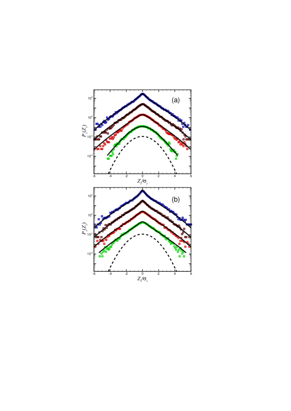
Figure 1: Continuous deformation of the increments’ PDFs in log-linear scale, for the $M=7.1$ earthquake across scales for, from top to bottom, $s=200,\;400,\;600,$ and 800 ms, and (a) far from, and (b) close to, the earthquake. Solid curves are the PDFs based on Eq. (2), while dashed curves are the Gaussian PDF.

To fit the increments’ PDF to Eq. (2), we estimate the variance $\lambda^{2}_{s}(s)$, using the least-squares method, with the error bars estimated by the goodness of the fit method. Deviation of $\lambda^{2}_{s}(s)$ from zero is a possible indicator of non-Gaussian statistics. As shown in Fig. 1, we find an accurate parametrization of the PDFs by $\lambda^{2}_{s}(s)$ for both data sets. Moreover, the PDF of $Z_{s}$ for the data set (I) becomes essentially Gaussian as $s$ increases to 800 ms, whereas it deviates from the Gaussian distribution for the data set (II). The time scale $s=800$ ms for $\lambda_{s}^{2}$ within a moving window was estimated by the plot of $\lambda_{s}^{2}$ vs $s$ for the data set (I) (background fluctuations), and selecting $s$ such that $\lambda_{s}\to 0$ (see also below).

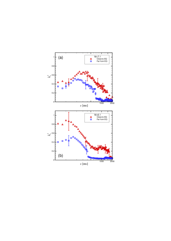
Figure 2: Scale-dependence of $\lambda_{s}^{2}$ vs $\log s$. (a) The $M=7.1$ event, both far from [data set (I)] and close to [data set (II)] the earthquake. For the data set (I) and $s>700$ ms, $\lambda_{s}^{2}\to 0$, implying that the increments’ PDF is Gaussian, whereas for the data set (II) $\lambda_{s}^{2}$ deviates strongly from zero for $700\;{\rm ms}<s<1500$ ms. (b) Same as in (a), but for the $M=6.1$ earthquake. When $\lambda_{s}\to 0$ the error bars are very small, about the same size as the symbols.

The scale-dependence of the parameter $\lambda_{s}^{2}$ of the PDF is shown in Fig. 2. For the data set (I) of the $M=7.1$ earthquake, shown in Fig. 2(a), and times $200\;{\rm ms}<s<500\;{\rm ms}$, a logarithmic decay, $\lambda^{2}_{s}\propto\log s$, is obtained. For the data set (II), the logarithmic regime extends to $300\;{\rm ms}<s<2000\;{\rm ms}$. Figure 2(b) presents similar behavior for the $M=6.1$ earthquake. We note that, for the data set (II) of the $M=6.1$ earthquake, there is a crossover time at which $\lambda_{s}^{2}$ changes from a $\sim\log(s)$ behavior to having a finite value, $\simeq 0.3$.

The importance of the results shown in Fig. 2 is that, they indicate that the increments’ PDFs for $s>2000$ ms and $s>1500$ ms are almost Gaussian ($\lambda_{s}^{2}\to 0$) for the $M=7.1$ and $M=6.1$ earthquakes [for the data set (II)], respectively. Transforming the time scales to length scales via the velocity of the elastic waves in Earth, $\sim 5000$ m/sec, the corresponding length scales are about 10 km and 7.5 km, for the same earthquakes, respectively, implying that larger earthquakes have larger characteristic length scales, and that for the $M=6.1$ event, there is a smaller active part in the fault.

We note that as one moves down the cascade process from the large to small scales, one expects the statistics to increasingly deviate from Gaussianity (see above and Fig. 2), in order to derive Eq. (2). Note that, a non-Gaussian PDF with fat tails on small scales indicates an increased probability of the occurrence of short-time extreme seismic fluctuations.

From the point of view of the increments’ PDF, the non-Gaussian noise with uncorrelated $\omega_{s}$ in the process, $Z_{s}(t)=\zeta_{s}(t)\exp[\omega_{s}(t)]$, and a multifractal formulation are indistinguishable, because their one-point statistics at any given scale may be identical. Thus, to understand the origin of the non-Gaussian fluctuations, we explore the correlation properties of $\omega_{s}$. To do so, we use an alternative method for studying the correlation functions of the local “energy” fluctuations [20]. We define the magnitude of local variance over a scale $s$ by, $\sigma_{s}^{2}(t)_{s}^{-1}\sum^{n_{s}/2}_{k=-n_{s}/2}Z_{s}(t+k\Delta t)^{2}$, and, $\bar{\omega}_{s}(i)=\frac{1}{2}\log\sigma_{s}^{2}(i)$, respectively. Here, $\Delta t$ is the sampling interval and, $n_{s}\equiv s/\Delta t$. The magnitude of the correlation function of $\bar{\omega_{s}}$ is then defined by

$$C^{(s)}(\tau)=\langle[\bar{\omega}_{s}(t)-\langle\bar{\omega}_{s}\rangle][\bar{\omega}_{s}(t+\tau)-\langle\bar{\omega}_{s}\rangle]\rangle\;,$$ (3)

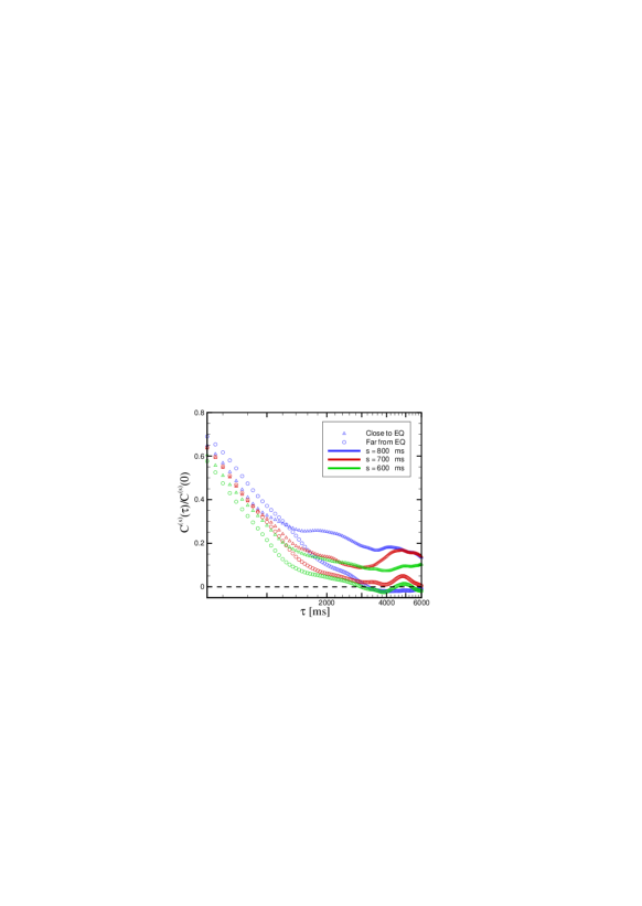
Figure 3: The correlation function $C^{(s)}(\tau)$ for the data set (I) far from, and the set (II) close to, the $M=7.1$ earthquake.

where $\langle\cdot\rangle$ indicates a statistical average. Figure 3 shows the results for the two data sets. The correlation function decays sharply for the data set (I) - far from the earthquakes - whereas it is of long-range type for the set (II) - close to the earthquakes.

We emphasize that for the data set (II), the PDF deviates from being Gaussian even for $s>800$ ms. Although one might argue that the deviations might be due to an underlying Lévy statistics, this possibility is ruled out due to the deduced hierarchical structures that imply that the increments for different scales are not independent; see Fig 3.

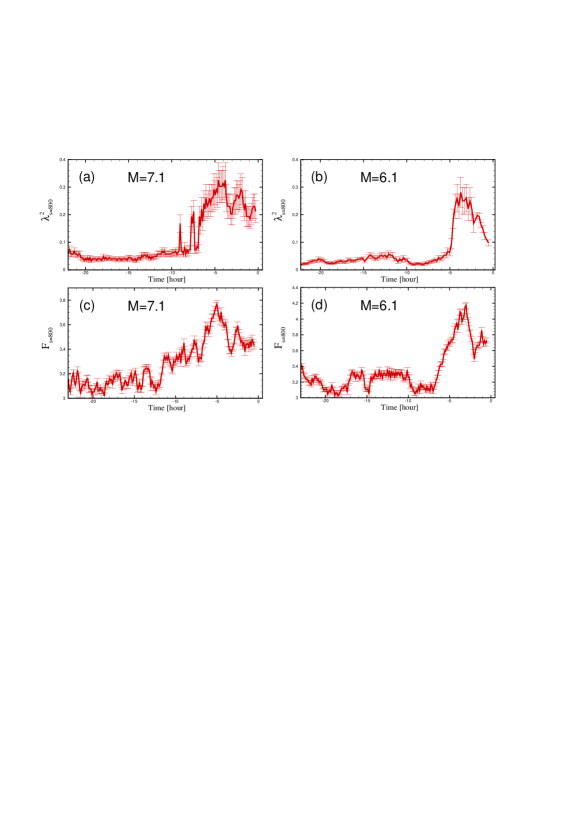
Figure 4: The local temporal dependance of $\lambda^{2}_{s}$ and the flatness for $s=800$ ms, over a one-hour period, for the $M=7.1$ and $M=6.1$ events, indicating a gradual, systematic increase on approaching the earthquakes.

We now show that the analysis may be used as a new precursor for detecting an impending earthquake. A window containing one hour of data is selected and moved with $\Delta t=15$ minutes to determine the temporal dependence of $\lambda_{s}^{2}$. Guided by Fig. 2, the local temporal variations of $\lambda_{s}^{2}$ for $s=800$ ms are investigated. According to Fig. 2, for $s\simeq 800$ ms, the difference between the values of $\lambda^{2}$ is large enough for the background data and the data set near the earthquakes. Hence, such a time scale may be used as the characteristic time for the dynamics of the non-Gaussian indicator $\lambda_{s}^{2}$. Figures 4(a) and 4(b) display a well-pronounced, systematic increase in $\lambda_{s}^{2}$ as the earthquakes are approached. Taking into account the estimated error of $\lambda_{s}^{2}$ for the background fluctuations in Figs. 4, we see that about 7 and 5 hours before the earthquakes values of $\lambda_{s}^{2}$ are larger, by more than two standard deviations, than those for the background.

We note that in defining $\lambda_{s}$, one supposes that the PDF of the increments is log-normal. This may induce errors due to the fact that, one must fit the PDF with a predefined functional form. An unbiased quantity that measures the intermittency and deviation from Gaussian is the flatness, which provides an unbiased estimator of deviations from Gaussianity, without having to adopt a priori any functional form for the PDF. In Figs. 4(c) and 4(d) we present the flatness of the time series in the same windows (see above) for time scale $s\simeq 800$ ms. They show that, consistent with $\lambda_{s}^{2}$, the flatness also yields a clear alert for an impending earthquake.

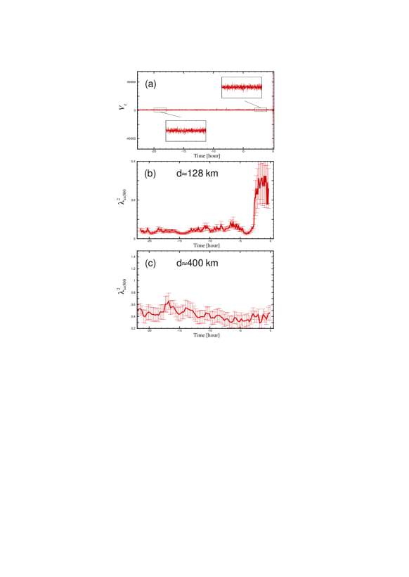
Figure 5: (a) The data for the $M=5.4$ earthquake in California. (b) and (c) Show the local temporal dependance of $\lambda^{2}_{s}$ for $s=500$ ms, collected at stations with a distance $d$ from the epicenter. The station at $d=$ 128 km provides the alert, whereas the second station does not yield any alert.

Due to the localization of elastic waves in Earth, stations that are far from an earthquake epicenter cannot provide any clue to the transition in the shape of the increments’ PDF. We checked this point for several earthquakes. Shown in Fig. 5 are the results for the $M=5.4$ California earthquake, occurred at (40.837 N, 123.499 W). The distance from the epicenter of the station that does provide an alert of about 3 hours for the earthquake is about $\simeq 128$ km, while the second station that does not yield any alert is about $\simeq 400$ km from the epicenter.

We also analyzed several other earthquakes of various magnitudes. We found that for earthquakes with $M\leq 5$ the increase in $\lambda_{s}^{2}$ is not large, even for the data that are collected in stations about 100 km from the epicenters. Moreover, we also analyzed seismic data for large earthquakes in Pakistan and Iran, and found that they exhibit the same types of trends and results, as those presented above, for the time variation of $\lambda_{s}^{2}$ close to the earthquakes. For example, for the $M=7.6$ earthquake that occurred on August 10, 2005, in Pakistan, the transition in the value of $\lambda_{s}^{2}$ occurred about 10 hours before the earthquake, while for the $M=6.3$ earthquake that occurred in northern Iran on May 28, 2004, the transition happened about 4 hours before the earthquake.

In summary, the temporal dependence of the fat tails of the PDF of the increments of the vertical velocity $V_{z}(t)$ of Earth exhibits a gradual, systematic increase in the probability of the appearance of large values on approaching a large or moderate earthquake, which is interpreted as an alert for the earthquake. To estimate the alert time one must, (i) utilize the time series $V_{z}(t)$, collected at broad-band stations near the epicenters. Due to localization of elastic waves in rock [15], data from far away stations cannot provide any clue to the transition in the shape of the increments’ PDF. The station’s distance (300 km) is not universal and depends on the geology, but it is of the correct order of magnitude. (ii) The time scale $s$ for moving $\lambda_{s}^{2}$ (here, 800 ms) is estimated by its plot vs $s$ for data set (I), and a choice of $s$ such that $\lambda^{2}\to 0$. On this scale the difference between $\lambda_{s}^{2}$ for the data sets (I) and (II) will be large enough to obtain a meaningful alert for the earthquake. (iii) One must also estimate $\lambda_{s}^{2}$ or the flatness in some windows (here, 1 hour windows) and move it over the time series, in order to observe its variations with the time.

We thank R. Friedrich, U. Frisch, H. Kantz, and K. R. Sreenivasan for critical reading of the manuscript, as well as J. G. Jim$\acute{e}$nez, T. Matsumoto, M. Mokhtari and S. M. Movahed for useful discussions. M.R.R.T. would like to thank the Alexander von Humboldt Foundation, the Associate program of the Abdus Salam International Center for Theoretical Physics, and the Knowledge Archive funding for financial support. The data for $V_{z}(t)$ were provided by the USGS and the National Geographic Institute of Spain.

• Modelling Critical and Catastrophic Phenomena in Geoscience: A Statistical Physics Approach, edited by P. Bhattacharyya and B. K. Chakrabarti, Lecture Notes in Physics 705 (Springer, Berlin, 2006).

• B. Gutenberg and R. F. Richter, Seismicity of the Earth (Hafner Publishing, New York, 1965).

• T. Utsu, Y. Ogata, and R. S. Matsu’ura, J. Phys. Earth 43, 1 (1995).

• P. Bak and C. Tang, J. Geophys. Res. 94, 15635 (1989).

• M. Sahimi, M. C. Robertoson, and C. G. Sammis, Phys. Rev. Lett. 70, 2186 (1993); H. Nakanishi et al., Phys. I 3, 733 (1993), M. C. Robertson et al., J. Geophys. Res. B 100, 609 (1995).

• S. Hallerberg, E. G. Altmann, D. Holstein, and H. Kantz, Phys. Rev. E 75, 016706 (2007); S. Hallerberg and H. Kantz, ibid. 77, 011108 (2008).

• D. D. Jackson, Proc. Natl. Acad. Sci. USA 93, 3772 (1996).

• M. R. Rahimi Tabar, M. Sahimi, K. Kaviani et al., in Ref. [1], p. 281.

• F. Mormann et al., Clin. Neurophysiol. 116, 569 (2005).

• A. Johansen and D. Sornette, Eur. Phys. J. B 1, 141 (1998).

• N. Vandewalle et al., Eur. Phys. J. B 4, 139 (1998).

• D. Sornette, Proc. Natl. Acad. Sci. USA 99, 2522 (2002).

• E. Larose, L. Margerin, B. A. vanTiggelen, M. Campillo, Phys. Rev. Lett. 93, 048501 (2004); N. M. Shapiro et al., Science 307 (2005).

• F. Shahbazi, A. Bahraminasab, S. M. Vaez Allaei, M. Sahimi, and M. R. Tabar, Phys. Rev. Lett. 94, 165505 (2005); A. Bahraminasab, S. M. Allaei, F. Shahbazi, M. Sahimi, M. D. Niry, M. R. Tabar, Phys. Rev. B 75, 064301 (2007); R. Sepehrinia, A. Bahraminasab, M. Sahimi, M. R. Tabar, ibid. 77, 014203 (2008); S. M. Vaez Allaei, M. Sahimi, and M. R. Rahimi Tabar, J. Stat. Mech. (2008) P03016.

• K. Kiyono et al., Phys. Rev. Lett. 93, 178103 (2004).

• K. Kiyono, Z. R Struzik, N. Aoyagi, F. Togo, Y. Yamamoto, Phys. Rev. Lett. 95, 058101 (2005).

• K. Kiyono, Z. R. Struzik, and Y. Yamamoto, Phys. Rev. Lett. 96, 068701 (2006); Phys. Rev. E 76, 041113 (2007); G. R. Jafari, et al., Int. J. Mod. Phys. C 18, 1689 (2007).

• U. Frisch and D. Sornette, J. Phys. I (France) 7, 1155 (1997).

• J. F. Muzy, J. Delour, and E. Bacry, Eur. Phys. J. B 17 537 (2000).

• A. Arneodo, E. Bacry, S. Manneville, J. F. Muzy, Phys. Rev. Lett. 80, 708 (1998).

• B. Castaing, Y. Gagne, and E. J. Hopfinger, Physica D 46, 177 (1990).

• B. Dubrulle, Phys. Rev. Lett. 73 959 (1994); Z.-S. She and E. C. Waymire, ibid. 74 262 (1995).

• B. Chabaud et al., Phys. Rev. Lett. 73, 3227 (1994).

• H. E. Stanley and V. Plerou, Quant. Fin. 1, 563 (2001).

• S. Ghashghaie, W. Breymann, J. Peinke, P. Talkner, and Y. Dodge, Nature 381, 767 (1996).

• P. A. Varotsos, N. V. Sarlis, H. K. Tanaka, E. S. Skordas, Phys. Rev. E 72, 041103 (2005).

• M. De Menecha and A. L. Stella, Physica A 309, 289 (2002).

• F. Caruso, A. Pluchino, V. Latora, S. Vinciguerra, A. Rapisarda, Phys. Rev. E 75, 055101(R) (2007).