Entropic stochastic resonance: the constructive role of the unevenness

Abstract

We demonstrate the existence of stochastic resonance (SR) in confined systems arising from entropy variations associated to the presence of irregular boundaries. When the motion of a Brownian particle is constrained to a region with uneven boundaries, the presence of a periodic input may give rise to a peak in the spectral amplification factor and therefore to the appearance of the SR phenomenon. We have proved that the amplification factor depends on the shape of the region through which the particle moves and that by adjusting its characteristic geometric parameters one may optimize the response of the system. The situation in which the appearance of such entropic stochastic resonance (ESR) occurs is common for small-scale systems in which confinement and noise play an prominent role. The novel mechanism found could thus constitute an important tool for the characterization of these systems and can put to use for controlling their basic properties.

1 Introduction

A Brownian particle moving in a threshold-like potential landscape and subjected to the influence of a periodic forcing may exhibit a coherent response giving rise to an amplification of the input at a certain optimal value of the noise level. This resonant phenomenon, observed in general in the wide class of periodically modulated noisy systems, was termed stochastic resonance and constituted a paradigm shift in the way we think about noise effects in systems away from equilibrium gammaitoni . In this new paradigm, the presence of noise does not always constitute a nuisance; on the contrary, it may play a constructive role gammaitoni ; bulsaraJS ; PT_SR ; chemphyschem ; vilar_mono ; Lutz99 ; Schmid01 ; BuchSR ; Yasuda08 ; scholarpediaSR ; GoychukSRa ; GoychukSRb .

Up to now, the phenomenon of SR has been observed mainly in systems dominated by the presence of a purely energetic potential or possessing some dynamical threshold gammaitoni . However, when scaling down the size of a system, the free energy rather than the internal energy becomes the most appropriate potential, and there are cases in which changes in the free energy are mainly due to entropy variations GoychukSRa ; hille ; zeolites ; liu ; berzhkovski ; Reguera_PRL ; Burada_PRL . This is what occurs in constrained systems. In the case of a Brownian particle moving in a confined medium, entropy variations contribute to changes in the free energy and may under some circumstances become its leading contribution GoychukSRb ; hille ; Reguera_PRL ; Burada_PRL . We will show in this work that the unevenness may also give rise to a stochastic resonance effect and that this effect can be controlled upon variation of the geometrical parameters, characterizing the shape of the cavity in which the Brownian particle dwells.

Usually, the analysis of SR effects have been performed by means of pertinent Langevin or corresponding Fokker-Planck models hanggithomas ; Risken . In confined systems the presence of boundaries exerts a strong influence in the dynamics and one has to solve the corresponding boundary value problem. This task cannot always be easily achieved. The fact that in many instances boundaries are very intricate enormously complicates the mathematical treatment of the problem to the extent of becoming a Herculean task when the boundaries are extremely irregular Burada_PRE . This feature demands the implementation of different approaches entailing a simplification of the analysis Jacobs ; Zwanzig ; Reguera_PRE . Among them, the Fick-Jacobs equation, based on a coarsening of the description in terms of a single, relevant coordinate degree of freedom, accurately performs this task Reguera_PRL ; Burada_PRL ; Burada_PRE ; Jacobs ; Zwanzig . This methodology will guide us in this article to analyze the appearance of the SR effect in presence of unevenness.

The article is organized in the following way. In Section 2, we introduce a model for Brownian motion in a confined medium. In Section 3, we present a reduction method which simplifies the complex nature of the 3D/2D dynamics giving rise to an effective one-dimensional kinetic description. Section 4 is devoted to evaluate the transition rate from the reduced kinetic description, and the introduction of spectral amplification within the two-state approximation. In Section 5, we present the results showing the ESR phenomenon. The impact of the geometrical shape and confinement on the spectral amplification is discussed in Section 6. Finally, we summarize our main conclusions in Section 7.

2 Confined Brownian motion

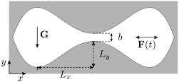
Figure 1: Schematic illustration of the two-dimensional structure confining the motion of the Brownian particles. The symmetric structure is defined by a quartic double well function, cf. Eq. (2), involving the geometrical parameters $L_{x}$, $L_{y}$ and $b$. Brownian particles are driven by a sinusoidal force $\vec{F}(t)$ along the longitudinal direction and a constant force $\vec{G}$ in the orthogonal direction.

The dynamics of a particle in a constrained geometry subjected to a sinusoidal oscillating force $F(t)$ along the axis of the structure and to a constant force $G$ acting along the orthogonal, or transverse, direction can be described by means of the Langevin equation written, in the overdamped limit, as

$$\gamma\,\frac{\mathrm{d}\vec{r}}{\mathrm{d}t}=-G\vec{e_{y}}-F(t)\vec{e_{x}}+\sqrt{\gamma\,k_{\mathrm{B}}T}\,\vec{\xi}(t)\,,$$ (1)

where $\vec{r}$ denotes the position of the particle, $\gamma$ is the friction coefficient, $\vec{e_{x}}$ and $\vec{e_{y}}$ the unit vectors along $x$ and $y$-directions, respectively, and $\vec{\xi}(t)$ is a Gaussian white noise with zero mean which obeys the fluctuation-dissipation relation $\langle\xi_{i}(t)\,\xi_{j}(t^{\prime})\rangle=2\,\delta_{ij}\,\delta(t-t^{\prime})$ for $i,j=x,y$. The explicit form of the longitudinal force is given by $F(t)=F_{0}\sin(\Omega t)$ where $F_{0}$ is the amplitude and $\Omega$ is the angular frequency of the sinusoidal driving.

In the presence of confinement, this equation has to be solved by imposing reflecting (no-flow) boundary conditions at the walls of the structure. For the 2D structure depicted in Fig. 1, the walls are defined by

$$w_{\mathrm{l}}(x) =L_{y}\left(\frac{x}{L_{x}}\right)^{4}-2\,L_{y}\left(\frac{x}{L_{x}}\right)^{2}-\frac{b}{2}\,=-w_{\mathrm{u}}(x)\,,$$ (2)

where $w_{\mathrm{l}}$ and $w_{\mathrm{u}}$ correspond to the lower and upper boundary functions, respectively. The characteristic length $L_{x}$ refers to the distance between the bottleneck and the position of maximal width, $L_{y}$ corresponds to the narrowing of the boundary functions and $b$ to the remaining width at the bottleneck, cf. Fig. 1. Consequently, the local width of the structure reads: $2\,w(x)=w_{\mathrm{u}}(x)-w_{\mathrm{l}}(x)$. This particular choice of the geometry is intended to resemble the classical setup for SR in the context of energetic barriers. In fact, in the limit of a sufficiently large transverse force $G$, the particle is in practice restricted to explore the region very close to the lower boundary of the structure, recovering the effect of an energetic bistable potential. For the sake of a dimensionless description, we measure all lengths in units of $L_{x}$, i.e. ${\tilde{x}}=x/L_{x}$, $\tilde{y}=y/L_{x}$ implying ${\tilde{b}}=b/L_{x}$ and ${\tilde{w}}_{\mathrm{l}}=w_{\mathrm{l}}/L_{x}=-{\tilde{w}}_{\mathrm{u}}$, temperature in units of an arbitrary, but irrelevant reference temperature $T_{\mathrm{R}}$ and time in units of $\tau=\gamma L_{x}^{2}/k_{\mathrm{B}}T_{\mathrm{R}}$, that is, twice the time the particle takes to diffuse a distance $L_{x}$ at temperature $T_{\mathrm{R}}$, i.e. ${\tilde{t}}=t/\tau$ and $\tilde{\Omega}=\Omega\tau$. We scale forces by $F_{\mathrm{R}}=\gamma L_{x}/\tau$, i.e. the orthogonal force reads ${\tilde{G}}=G/F_{\mathrm{R}}$ and the sinusoidal force ${\tilde{F}(\tilde{t})}=F(t)/F_{\mathrm{R}}$. For better legibility, we shall omit the tilde symbols in the following. In dimensionless form the Langevin-equation (1) and the boundary functions (2) read:

$$\frac{\mathrm{d}\vec{r}}{\mathrm{d}t} =-G\vec{e_{y}}-F(t)\vec{e_{x}}+\sqrt{D}\,\vec{\xi}(t)\,,$$ (3)

$$w_{\mathrm{l}}(x) =-w_{\mathrm{u}}(x)=\epsilon x^{4}-2\epsilon x^{2}-b/2\,,$$ (4)

where we defined the aspect ratio $\epsilon=L_{y}/L_{x}$ and the rescaled temperature $D=T/T_{\mathrm{R}}$.

3 Reduction of dimensionality

Since the above mentioned dynamics given by Eq. (3) with the boundary conditions could not be solved analytically, we simplified the problem by assuming equilibration in $y$- direction and thereby reducing the dimensionality of the problem Jacobs ; Zwanzig ; Reguera_PRE ; Percus .

First, we consider the case in the absence of the periodic forcing, i.e. $F(t)=0$. Then, the 2D dynamics is described by the following 2D Smoluchowski equation Risken ; hanggithomas

$$\frac{\partial}{\partial t}P(x,y,t)=D\frac{\partial}{\partial x}e^{-U(x,y)/D}\frac{\partial}{\partial x}e^{U(x,y)/D}P(x,y,t)\,\\ +D\frac{\partial}{\partial y}e^{-U(x,y)/D}\frac{\partial}{\partial y}e^{U(x,y)/D}P(x,y,t)\,,$$ (5)

with reflecting boundary conditions at the confining walls and where the potential function is given by $U(x,y)=G\,y$. Since we are mainly interested in the dynamics in $x$-direction, we introduce the marginal probability density $P(x,t)$ which is obtained by integration over the transverse coordinate:

$$P(x,t)=\int\mathrm{d}y\,P(x,y,t)\,.$$ (6)

On integrating Eq. (5) over the transverse direction, we get

$$\frac{\partial}{\partial t}P(x,t)=\\ D\frac{\partial}{\partial x}\int\,\mathrm{d}y\,\left\{e^{-U(x,y)/D}\frac{\partial}{\partial x}e^{U(x,y)/D}P(x,y,t)\right\}\,.$$ (7)

Assuming local equilibrium in the $y$-direction, we define the $x$-dependent effective energy function $A(x)$ (omitting irrelevant constants) reading

$$e^{-A(x)/D}=\int\mathrm{d}y\,e^{-U(x,y)/D}\,.$$ (8)

Consequently, the conditional local equilibrium probability distribution of $y$ at a given $x$ becomes

$$\rho(y;x)=e^{-U(x,y)/D}\,e^{A(x)/D}\,,$$ (9)

and is normalized for every $x$. As a result, the two dimensional probability distribution can be approximately expressed as

$$P(x,y,t)\cong P(x,t)\rho(y;x)\,,$$ (10)

and the kinetic equation for the marginal probability distribution, cf. Eq. (7), becomes

$$\frac{\partial}{\partial t}P(x,t)\cong D\frac{\partial}{\partial x}e^{-A(x)/D}\frac{\partial}{\partial x}e^{A(x)/D}P(x,t)\,.$$ (11)

In the present case with a constant force $G$ in the negative $y$-direction the potential function $A(x)$ reads, cf. Eq. (8):

$$A(x) =-D\ln\left[\int_{w_{\mathrm{l}}(x)}^{w_{\mathrm{u}}(x)}\,e^{-G\,y/D}\,\mathrm{d}y\right]$$

$$=-D\ln\left[\frac{D}{G}\left(e^{-Gw_{\mathrm{l}}(x)/D}-e^{-Gw_{\mathrm{u}}(x)/D}\right)\right]\,.$$ (12)

Making use of the symmetry of our considered structure, i.e. $w_{\mathrm{u}}(x)=-w_{\mathrm{l}}(x)$ and the definition of the half width function $w(x)=(w_{\mathrm{u}}-w_{\mathrm{l}})/2$, the potential function turns into

$$A(x)=-D\,\ln\left[\frac{2D}{G}\,\sinh\left(\frac{Gw(x)}{D}\right)\,\right]\,.$$ (13)

Eq. (11) can then be rewritten as

$$\frac{\partial P(x,t)}{\partial t}=\frac{\partial}{\partial x}\left\{D\frac{\partial P}{\partial x}\,+A^{\prime}(x)\,P\right\}\,,$$ (14)

with the potential function $A(x)$ given by Eq. (3) (or by Eq. (13) for $w_{\mathrm{l}}(x)=-w_{\mathrm{u}}(x)$) and with the prime referring to the derivative with respect to $x$. In general, after the coarse-graining the diffusion coefficient will depend on the coordinate $x$, but since in our case $|w^{\prime}(x)|\ll 1$, the correction can be safely neglected Burada_PRE ; Zwanzig ; Reguera_PRE ; Percus ; Berezhkovskii2007 .

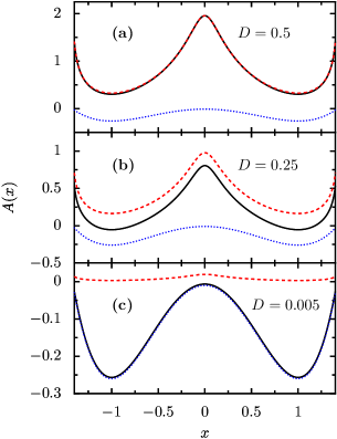
Figure 2: (Color online) The effective 1D potential $A(x)$ is depicted (solid black line) for $G=1$ and for different noise strengths. For comparison the potential functions for the pure energetic case (dotted blue line), i.e. $A(x)=Gw_{\mathrm{l}}(x)$, and for the pure entropic case (dashed red line), i.e. $A(x)=-D\ln[2w(x)]$, are plotted as well.

It is important to highlight that the potential $A(x)$ was not present in the 2D Langevin dynamics, but arises due to the entropic restrictions associated to the confinement. Then, equation (14) describes the motion of a Brownian particle in a free energy potential of entropic nature, as $A(x)$ does not only depend on the energetic contribution of the force $G$, but also on the temperature $D$ and the geometry of the structure in a non-trivial way. For a structure like that depicted in Fig. 1, the free energy $A(x)$ forms a double-well potential, cf. Fig. 2. As the width at the bottleneck of the channel approaches zero, the potential $A(x)$ diverges.

It is worth to analyze the two limiting situations that can be obtained depending on the transverse force $G$.

Energy-dominated situation:

For $G\gg 1$, Eq. (13) yields $A(x)=Gw_{\mathrm{l}}(x)$ (neglecting irrelevant constants) and the 1D kinetic equation (14) becomes the standard Fokker-Planck equation for Brownian motion in a purely energetic potential whose shape resembles the lower boundary of the structure,

$$\frac{\partial P(x,t)}{\partial t}=\frac{\partial}{\partial x}\left\{D\frac{\partial P(x,t)}{\partial x}+Gw_{\mathrm{l}}^{\prime}(x)P(x,t)\right\}\,.$$ (15)

Entropy-dominated situation:

In the opposite limit,
i.e. for $G\ll 1$, the effective potential is dominated by the purely entropic contribution $A(x)=-D\,\ln[2\,w(x)]$ and the kinetic equation turns into the Fick-Jacobs equation Jacobs ,

$$\frac{\partial P(x,t)}{\partial t}=\frac{\partial}{\partial x}\bigg{\{}D\frac{\partial P(x,t)}{\partial x}-D\frac{w^{\prime}(x)}{w(x)}P(x,t)\bigg{\}}\,.$$ (16)

4 Two-State approximation

It is instructive to analyze the occurrence of stochastic resonance in the context of the two-state approximation McNamara . Accordingly, the 1D kinetics given by Eq. (14) can be approximately mapped into a two-state system with the two states corresponding to the two wells of the symmetric effective potential $A(x)$. An estimate for the transition rates could be obtained by applying the Mean-First-Passage-Time (MFPT) approach hanggi .

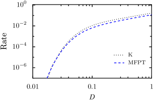
Figure 3: (Color online) The transition rate for the escape from one basin to the other obtained after applying a Two-State approximation of the 1D problem, cf. Eq. (17) and Eq. (21), is depicted as a function of the thermal noise $D$ for $G=1.0$. The 2D structure is defined by the boundary function given in Eq. (4) with $\epsilon=1/4$ and $b=0.02$. Here, the Kramers-Smoluchowski rate ($K$), i.e. $r_{\mathrm{K}}$, converges to the rate given by the inverse mean first passage time (MFPT) in the low noise limit.

4.1 Mean First Passage Time approach

In order to calculate the transition rate from one state to the other, one evaluates the inverse of the MFPT to reach a potential minimum after starting out from the other minimum of the symmetric and bistable potential $A(x)$. Then, the transition rate is given by

$$r_{\mathrm{MFPT}}(D,G)=\frac{1}{T_{1}(-1\to 1)}\,,$$ (17)

where $T_{1}(-1\to 1)$ is the first moment of the first passage time distribution for reaching $x=1$ starting out at $x=-1$. The $n$th moment of the first passage time distribution obeys the following recurrence relation hanggi

$$T_{n}(-1\to 1) :=\langle t^{n}(-1\to 1)\rangle$$

$$=\frac{n}{D}\int_{-1}^{1}\mathrm{d}x\,e^{A(x)/D}\int_{-\infty}^{x}\mathrm{d}y\,e^{-A(y)/D}$$

$$\times\langle t^{n-1}(y\to 1)\rangle$$ (18)

for $n\in\mathbb{N}$ and with $T_{0}(a\rightarrow b)=1$ for arbitrary a and b. Accordingly, within the one dimensional approximation, cf. Eq. (14), the mean first passage time (i.e., $n=1$) for the potential function $A(x)$, cf Eq. (13), reads

$$T_{1} =\frac{1}{D}\int_{-1}^{1}\mathrm{d}x\,e^{A(x)/D}\int_{-x_{\mathrm{l}}}^{x}\mathrm{d}y\,e^{-A(y)/D}$$

$$=\frac{1}{D}\int_{-1}^{1}\mathrm{d}x\,\mathrm{csch}\left(\frac{Gw(x)}{D}\right)\int_{-x_{\mathrm{l}}}^{x}\mathrm{d}y\,\sinh\left(\frac{Gw(y)}{D}\right)\,,$$ (19)

where $x_{\mathrm{l}}$ is the left limiting value at which the boundary function vanishes. Eq. (4.1) can be evaluated using a steepest descent approximation leading to the commonly known Kramers-Smoluchowski rate.

4.2 Kramers-Smoluchowski rate

For a potential $A(x)$ with a barrier height $\Delta A\gg D$ the escape rate of an overdamped Brownian particle from one well to the other in the presence of thermal noise, and in the absence of a force, is given by the Kramers-Smoluchowski rate McNamara ; hanggi ; kramers ; Jung91 , reading in dimensionless units,

$$r_{\mathrm{K}}(D)=\frac{\sqrt{A^{\prime\prime}(x_{\mathrm{min}})|A^{\prime\prime}(x_{\mathrm{max}})|}}{2\pi}\,\exp\left(\frac{-\Delta A}{D}\right)\,,$$ (20)

where $A^{\prime\prime}$ is the second derivative of the effective potential function with respect to $x$, and $x_{\mathrm{max}}$ and $x_{\mathrm{min}}$ indicate the position of the maximum and minimum of the symmetric potential, respectively.

For the potential given by Eq. (13) and the shape defined by Eq. (4), the corresponding Kramers-Smoluchowski rate for transitions from one basin to the other reads Burada_PRL

$$r_{\mathrm{K}}(D)=\frac{G\,\epsilon}{\pi}\,\frac{\sqrt{2\,\sinh\left(\frac{Gb}{D}\right)\,\sinh\left(\frac{G(b+2\epsilon)}{D}\right)}}{{\sinh}^{2}\left(\frac{G(b+2\epsilon)}{2D}\right)}$$ (21)

Note that the Kramers-Smoluchowski approximation yields good results for barrier heights $\Delta A$ much larger than the thermal energy that in the present scaling is given by $D$. In fact, for $\Delta A\gg D$ the Kramers-Smoluchowski rate $r_{\mathrm{K}}$ approximates accurately the rate $r_{\mathrm{MFPT}}$ evaluated numerically from the MFPT expression  (4.1), as depicted in Fig. 3.

5 Role of the transverse force $\vec{G}$

In section 3 we introduced the Fick-Jacobs equation to approximatively describe the Brownian motion in a 2D structure like that depicted in Fig. 1 using a simplified 1D modeling with an effective bistable potential. This potential exhibits a barrier the particle has to overcome noisily in order to make a transition from one well to the other. For a sinusoidal driving force applied in $x$-direction, i.e. $F(t)=F_{0}\,\sin(\Omega t)$, a synchronization effect between the oscillatory forcing and the noise-induced transitions over the entropic potential barrier takes place and was reported previously in Ref. Burada_PRL . Under these circumstances and in the presence of a finite orthogonal, i.e. transverse force $G$, increasing the noise level results in a noise-amplified response signal. The improvement of the response is quantified in the following by the spectral amplification factor $\eta$, which is the ratio of the power stored in the response of the system at the driving frequency $\Omega$ and the power of the sinusoidal driving signal. The occurrence of the Entropic Stochastic Resonance effect manifests in the presence of an optimal dose of noise for which the spectral amplification is maximal Burada_PRL .

5.1 Two-State modeling

It is straight forward to derive an analytic expression for the spectral amplification within a two-state modeling. The sinusoidal driving modulates the transition rates, which are given either by $r_{\mathrm{MFPT}}$ or $r_{\mathrm{K}}$ (cf. Sec. 4). Within a first order perturbation theory in the ratio of driving amplitude $F_{0}$ and noise level $D$, it is possible to find a closed expression for the response of the two-state system and accordingly for the spectral amplification factor that reads gammaitoni ; Jung91 :

$$\eta=\frac{1}{D^{2}}\,\frac{4\,r_{\mathrm{Rate}}^{2}(D)}{4\,r_{\mathrm{Rate}}^{2}(D)+\Omega^{2}}\,,$$ (22)

where $r_{\mathrm{Rate}}$ is the transition rate of the unperturbed two-state system and is given by Eq. (17), or approximately by Eq. (20).

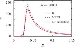
Figure 4: (Color online) A detailed comparison of the behavior of the spectral amplification factor obtained numerically from the 1D modeling (solid line), cf. Eq.(23) and Eq.(25), and within the two-state approximation (Eq.(22)), using either the Kramers-Smoluchowski rate (K) (dotted line) or the rate obtained directly from the mean first passage time (MFPT) (dashed-line). Here, the transverse force is $G=1.0$, and the structure is defined by Eq. (4) with an aspect ratio $\epsilon=1/4$, and a bottleneck width $b=0.02$.

5.2 1D modeling

Avoiding the approximations involved in the two-state modelling, the system’s response could also be obtained directly from the numerical integration of the 1D kinetic equation. In the presence of an oscillating force $F(t)$ in $x-$direction there is an additional contribution to the effective potential in Eq. (14) and the 1D kinetic equation in dimensionless units reads Burada_PRL

$$\frac{\partial P(x,t)}{\partial t}=\frac{\partial}{\partial x}\left\{D\frac{\partial P}{\partial x}+\textbf{(}A^{\prime}(x)-F(t)\textbf{)}\,P\right\}\,.$$ (23)

By spatial discretization, using a Chebyshev collocation method, and employing the method of lines, we reduced the kinetic equation to a system of ordinary differential equations, which was then solved using a backward differentiation formula method nag . As a result, we obtained the time dependent probability distribution $P(x,t)$ and, from that, the time-dependent average position defined as

$$\langle x(t)\rangle=\int x\,P(x,t)\mathrm{d}x\,,$$ (24)

which was computed in the long-time limit. After a Fourier-expansion of $\langle x(t)\rangle$ one finds the amplitude $M_{1}$ of the first harmonic of the system’s response. Hence, the spectral amplification $\eta$ Jung91 for the fundamental oscillation is evaluated as

$$\eta=\left[\frac{M_{1}}{F_{0}}\right]^{2}\,.$$ (25)

The spectral amplification $\eta$ depicts a bell-shaped behavior, cf. Fig. 4, indicating the existence of a Stochastic Resonance effect: there is a maximum of the spectral amplification at an optimal value of noise. The qualitative behavior is captured by the two-state approximation as well. The prediction of the two-state modelling with rates evaluated directly from MFPT is closer to the 1D modelling than those obtained by making use of the Kramers-Smoluchowski approximated rate, as illustrated in Fig. 4. This is due to the fact that the condition $\Delta A\gg D$ is not always fulfilled in this case. In fact for the entropy-dominated situation, $\Delta A$ and $D$ are of the same order of magnitude.

Next we present the results of numerical simulations of the full (2D) problem. By doing so we demonstrate that the ESR effect is robust and not just an artifact of the reduction procedure.

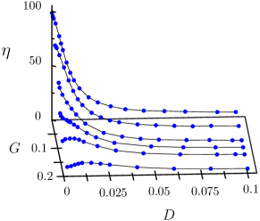
Figure 5: (Color online) The spectral amplification obtained from 2D simulations is depicted as a function of both the transverse force $G$ and the noise strength $D$ for an input signal frequency $\Omega=0.1$ and amplitude $F_{0}=0.1$. The shape of the two-dimensional channel is defined by the dimensionless function $w(x)=-\epsilon x^{4}+2\,\epsilon x^{2}+b/2$ with the aspect ratio $\epsilon=1/4$ and bottleneck width $b=0.02$. The symbols connected by lines correspond to the same $G$-values. In particular, these are $G=0.0,\,0.05,\,0.1,\,0.125,\,0.15$ and $0.2$. In the deterministic limit, i.e $D\to 0$, the spectral amplification reaches a limiting value ($1/\Omega^{2}$) for $G=0$. For $G=0$ the effect of Entropic Stochastic Resonance disappears.

5.3 2D modelling

The accuracy of the reduced one-dimensional kinetic description can be examined by comparing the results with those obtained by Brownian dynamic simulations, performed by integration of the overdamped 2D Langevin equation (1). The simulations were carried out using the standard stochastic Euler-algorithm.

The resulting amplification factor as a function of the value of the transverse force and the noise strength are plotted in Fig. 5. For a finite transverse force $G$ the spectral amplification exhibits a peak at an optimum value of the noise strength which is indicative of the effect of Entropic Stochastic Resonance. However, for vanishing transverse force $G$ the spectral amplification does not exhibit any peak and decays monotonically with increasing noise level, i.e. the ESR - effect is not observed. In the deterministic limit, i.e. $D\to 0$, the spectral amplification reaches the limit value $\eta=1/\Omega^{2}$ for $G=0$, as shown in Fig. 5. We remark that the later is only true when the amplitude of the system’s response, which is the ratio of input signal amplitude to input signal frequency, is smaller than the value $x_{l}$, which is the limiting value at which the boundary function vanishes. It is also worth to point out that starting out from a finite $G$-value the position of the ESR peak shifts towards smaller noise strengths as $G$ decreases while the maximum value increases, cf. Fig. 5. A comparison between the 1D-modelling and the full 2D simulation is depicted in Fig. 6. The 2D simulation results convincingly corroborate the validity of the modelling within the 1D Fick-Jacob approximation, see also below.

Thus, we detect a non-monotonic behavior of the spectral amplification only for finite values of the orthogonal force $G\neq 0$, while for $G=0$ the spectral amplification decays monotonically. In other words, for the dynamics and situation considered in Sec. 2 the occurrence of the ESR-effect requires a non-vanishing orthogonal force $G$ which contributes within the 1D modelling to the effective entropic potential.

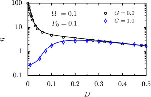
Figure 6: (color online) The dependence of the spectral amplification $\eta$ on noise level $D$, at two different values of the transverse force $G$, at a constant input frequency and amplitude. The symbols correspond to the results of the Langevin simulations for the two-dimensional channel whose shape is defined by $w(x)=-\epsilon x^{4}+2\,\epsilon x^{2}+0.01$ with an aspect ratio $\epsilon=1/4$, whereas the lines are the results of the numerical integration of the 1D kinetic equation (23). In the deterministic limit, i.e $D\to 0$, the spectral amplification reaches the limiting value ($1/\Omega^{2}$) for $G=0$.

6 Role of the shape of the structure

Fig. 6 depicts the main findings for the occurrence of the ESR-effect in an effective bistable configuration with two large basins connected by a small bottleneck, cf. Fig. 1. Namely: (i) the occurrence of the ESR-effect due to the interplay of a finite value of the orthogonal force $G$, and (ii) the ability of the 1D Fick-Jacobs approximation to reproduce very accurately the results of the full 2D problem Burada_PRE ; Burada_PRL .

Figure 7: Schematic illustration of the two-dimensional structure confining the motion of the Brownian particles. The shape defined by the dimensionless function $w(x)=12.5x^{8}-27.5x^{6}+18.21x^{4}-3.92x^{2}-0.01$.

Next, in order to investigate the impact of the shape of the structure on the ESR behavior we have considered yet another channel geometry: It is similar to the one depicted in Fig. 1 but exhibits two intermediate wider bottlenecks which are connected via a much narrower bottleneck, see in Fig. 7. The geometric shape of the structure is defined by the dimensionless width function

$$w(x)=12.5x^{8}-27.5x^{6}+18.21x^{4}-3.92x^{2}-0.01\,.$$ (26)

Following the same analysis performed in Sec. 5, we obtained the spectral amplification within the 1D modelling and compared it with results obtained from 2D numerical simulation of the Langevin equation (3) in the new 2D structure defined by Eq. (26). Again, the effective potential function $A(x)$ obtained from the Fick-Jacobs approximation exhibits a large potential barrier separating the two basins each of which is additionally separated by a smaller potential barrier into two wells. In fact, the construction of the alternative geometric structure was done in such a way to reveal the existence of a main entropic barrier controlling the transitions between the two main basins.

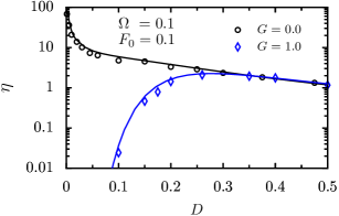
Figure 8: (Color online) The dependence of the spectral amplification $\eta$ on noise level $D$, at two different values of the transverse force $G$, at a constant input frequency and amplitude for the channel illustrated in Fig. 7). The symbols correspond to the results of the Langevin simulations for the two-dimensional structure whose shape is defined by $w(x)=12.5x^{8}-27.5x^{6}+18.21x^{4}-3.92x^{2}-0.01$, whereas the lines are the results of the numerical integration of the 1D kinetic equation (23). Like in Fig. 6, in the deterministic limit ($D\to 0$), the spectral amplification reaches the limiting value ($1/\Omega^{2}$) for $G=0$.

The behavior of spectral amplification as a function of the noise strength for the new channel defined by Eq. 26, and for two different values of the transverse force is depicted in Fig. 8. Interestingly, we can observe the existence of Entropic Stochastic Resonance even in the new structure, when the transverse force is present in the system. Comparing the results of Fig. 8 for the channel depicted in Fig. 7 with those in Fig. 6, one can observe that the ESR peak appears at higher values of the noise strength. In addition, the enhancement of the signal upon increasing the noise is more pronounced in the new structure. These results suggest that by a proper design of the geometry of the channel it would be possible to significantly enhance and optimize the response of a confined system. This would be specially important in biological systems, where the noise (i.e. the temperature) is a variable that can neither be arbitrarily chosen nor eliminated. Finally, it is also worth stressing that the Fick-Jacobs approximation still holds nicely in this case since the 2D numerical simulation results are in very good agreement with those obtained by 1D modelling.

Overall, the results indicate that the existence of a small bottleneck separating two basins and forming an effective entropic potential barrier, leads robustly to the occurrence of an Entropic Stochastic Resonance effect.

7 Conclusions

We have shown that unevenness may be the origin of many resonant phenomena in small-scale systems. The constrained motion of a Brownian particle in a region limited by irregular boundaries impedes the access of the particle to certain regions of space giving rise to entropic effects that can effectively control the dynamics. The interplay between the noise present in the system, the external modulation and the entropic effects results in an entropic stochastic resonance. However, the presence of a transverse force $G$ is crucial to observe this resonant behavior. This ESR is genuine of small scale systems where confinement yields entropic effects. The occurrence of ESR depends on the shape of the channel and can then be controlled by it. Thus understanding the role of noise and confinement in these systems does provide the possibility for a design of stylized channels wherein response and transport become efficiently optimized.

This work has been supported by the DFG via research center, SFB-486, project A10, the Volkswagen Foundation (project I/80424), the German Excellence Initiative via the Nanosystems Initiative Munich (NIM), and the DGCyT of the Spanish government through grant No. FIS2005-01299.

References

- (1) L. Gammaitoni, P. Hänggi, P. Jung, F. Marchesoni, Rev. Mod. Phys. 70, 223 (1998)
- (2) A. Bulsara, P. Hänggi, F. Marchesoni, F. Moss, M. Shlesinger, J. Stat. Phys. 70, 1 (1993)
- (3) A.R. Bulsara, L. Gammaitoni, Phys. Today 49 (3), 39 (1996)
- (4) P. Hänggi, ChemPhysChem 3, 285 (2002)
- (5) J.M.G. Vilar, J.M. Rubí, Phys. Rev. Lett. 77, 2863 (1996); J.M.G. Vilar, J.M. Rubí, Phys. Rev. Lett. 78, 2886 (1997)
- (6) V.S. Anishchenko, A.B. Neiman, F. Moss, L. Schimansky-Geier, Phys. Usp. 42, 7 (1999)
- (7) G. Schmid, I. Goychuk, P. Hänggi, Europhys. Lett. 56, 22 (2001)
- (8) T. Wellens, V. Shatokhin, A. Buchleitner, Rep. Prog. Phys. 67, 45 (2004)
- (9) H. Yasuda, T. Miyaoka, J. Horiguchi, A. Yasuda, P. Hänggi, Y. Yamamoto, Phys. Rev. Lett. 100, 118103 (2008)
- (10) C.R. Nicolis, G. Nicolis, Scholarpedia, 2(11), 1474 (2007)
- (11) I. Goychuk, P. Hänggi, Phys. Rev. Lett. 91, 070601 (2003)
- (12) I. Goychuk, P. Hänggi, J. L. Vega, S. Miret Artes, Phys. Rev. E 71, 061906 (2005)
- (13) B. Hille, Ion Channels of Excitable Membranes (Sinauer, Sunderland, 2001)
- (14) R.M. Barrer, Zeolites an Clay Minerals as Sorbents and Molecular Sieves (Academic Press, London, 1978)
- (15) L. Liu, P. Li, S.A. Asher, Nature 397, 141 (1999)
- (16) A.M. Berezhkovskii, S.M. Bezrukov, Biophys. J. 88, L17(2005)
- (17) D. Reguera, G. Schmid, P.S. Burada, J.M. Rubí, P. Reimann, P. Hänggi, Phys. Rev. Lett. 96, 130603 (2006)
- (18) P.S. Burada, G. Schmid, D. Reguera, M.H. Vainstein, J.M. Rubi, P. Hänggi, Phys. Rev. Lett. 101, 130602 (2008)
- (19) P. Hänggi, H. Thomas, Phys. Rep. 88, 207 (1982)
- (20) H. Risken, The Fokker-Planck equation, 2nd ed. (Springer, Berlin, 1989)
- (21) P.S. Burada, G. Schmid, D. Reguera, J.M. Rubí, P. Hänggi, Phys. Rev. E 75, 051111 (2007); P.S. Burada, G. Schmid, P. Talkner, P. Hänggi, D. Reguera, J.M. Rubí, BioSystems 93, 16 (2008)
- (22) M. H. Jacobs, Diffusion Processes (Springer, New York, 1967)
- (23) R. Zwanzig, J. Phys. Chem. 96, 3926 (1992)
- (24) D. Reguera, J.M. Rubí, Phys. Rev. E 64, 061106 (2001)
- (25) P. Kalinay, J.K. Percus, Phys. Rev. E 74, 041203 (2006)
- (26) A. M. Berezhkovskii, M.A. Pustovoit, S.M. Bezrukov, J. Chem. Phys. 126, 134706 (2007)
- (27) B. McNamara, K. Wiesenfeld, Phys. Rev. A 39, 4854 (1989)
- (28) P. Hänggi, P. Talkner, M. Borkovec, Rev. Mod. Phys. 62, 251 (1990)
- (29) H. Kramers, Physica (Utrecht) 7, 284 (1940)
- (30) P. Jung, P. Hänggi, Phys. Rev. A 44, 8032 (1991); ibid, Europhys. Lett. 8, 505 (1989)
- (31) NAG Fortran Library Manual, Mark 20 (The Numerical Algorithm Group Limited, Oxford, England, 2001)