CERN-PH-TH/2009-028

Estimating relic magnetic fields

from CMB temperature correlations

Massimo Giovannini

Department of Physics, Theory Division, CERN, 1211 Geneva 23, Switzerland
INFN, Section of Milan-Bicocca, 20126 Milan, Italy

Abstract

The temperature and polarization inhomogeneities of the Cosmic Microwave Background might bear the mark of pre-decoupling magnetism. The parameters of a putative magnetized background are hereby estimated from the observed temperature autocorrelation as well as from the measured temperature-polarization cross-correlation.

In recent years the observations of the Cosmic Microwave Background (CMB in what follows) have been translated into a set of constraints on the standard parameters of an underlying $\Lambda$CDM scenario where $\Lambda$ stands for the dark energy component (parametrized in terms of a cosmological constant) and CDM is the acronym of cold dark matter which is the dominant source of non-relativistic matter of the model. More specifically, the five year release of the WMAP data [1] (WMAP 5yr in what follows) can be used to infer the parameters of a putative $\Lambda$CDM paradigm where $\Omega_{X\,0}=\rho_{X0}/\rho_{\mathrm{crit}}$ denotes the (present) energy density of the species $X$ in units of the critical energy density $\rho_{\mathrm{crit}}$. The best-fit values of the $\Omega_{X0}$ as well as of the other parameters of the model can be determined, for instance, from the WMAP 5yr data alone (see also [2] for earlier results) and they are

$$\Omega_{\mathrm{b}0}=0.0441\pm 0.0030,\qquad\Omega_{\mathrm{c}0}=0.214\pm 0.027,\qquad\Omega_{\Lambda 0}=0.742\pm 0.030,$$ (1)

where the subscripts b and c stand, respectively, for baryons and CDM components; Eq. (1) does not exhaust the list of parameters which also include the Hubble constant (i.e. $H_{0}$), the optical depth of reionization (i.e. $\epsilon_{\mathrm{re}}$) and the spectral index of (adiabatic) curvature perturbations (i.e. $n_{\mathrm{s}}$):

$$H_{0}=71.9^{2.6}_{-2.7}\,\mathrm{km/sec}\,\mathrm{Mpc}^{-1},\qquad\epsilon_{\mathrm{re}}=0.087\pm 0.017,\qquad n_{\mathrm{s}}=0.963_{-0.015}^{0.014};$$ (2)

$\epsilon_{\mathrm{re}}$ corresponds, in the framework of the WMAP 5yr data, to a typical redshift $z_{\mathrm{re}}=11\pm 1.4$. In the $\Lambda$CDM paradigm the temperature and polarization inhomogeneities are solely sourced by the fluctuations of the spatial curvature ${\mathcal{R}}$ whose Fourier modes obey

$$\langle{\mathcal{R}}(\vec{k}){\mathcal{R}}(\vec{p})\rangle=\frac{2\pi^{2}}{k^{3}}\delta^{(3)}(\vec{k}+\vec{p}),\qquad{\mathcal{P}}_{{\mathcal{R}}}(k)={\mathcal{A}}_{\mathcal{R}}\biggl{(}\frac{k}{k_{\mathrm{p}}}\biggr{)}^{n_{\mathrm{s}}-1},$$ (3)

where ${\mathcal{A}}_{{\mathcal{R}}}=(2.41\pm 0.11)\times 10^{-9}$ is the amplitude of the curvature power spectrum at the pivot scale $k_{\mathrm{p}}=0.002\,\mathrm{Mpc}^{-1}$. The success of the $\Lambda$CDM paradigm suggests the possibility of constraining also other (non-standard) parameters such as a background of relic gravitons [1], non-adiabatic modes possibly present prior to equality [5] or even a background of relic magnetic fields whose presumed existence is not in contrast with the actual observations of large-scale magnetism in galaxies [6], clusters [7] or even (with mandatory caveats) in superclusters [8]. Can we falsify, at a given confidence level, the hypothesis that large-scale magnetic fields are already present prior to decoupling?

This paper follows a series of investigations [9] where large-scale magnetic fields have been consistently included at all the stages of the Boltzmann hierarchy and within a faithful plasma description incorporating the evolution of the space-time curvature and of its inhomogeneities. For frequencies smaller than the (electron) plasma frequency, the Ohmic current is solenoidal and the electric fields are suppressed by (Coulomb) conductivity: in this regime the effective dynamical variable is the centre of mass velocity of the electron ion fluid (sometimes named, with confusing terminology, the baryon velocity). For frequencies larger than the plasma frequency, the propagation of electromagnetic disturbances follows a two-fluid approach where ions and electrons are treated as independent dynamical entities: Faraday effect induces, in this regime, a B-mode polarization [10] which might be relevant when (and if) compelling experimental determinations of the B-mode autocorrelation will be available.

The temperature autocorrelations (TT spectra in what follows) and the temperature-polarization cross-correlations (TE spectra in what follows) are determined with reasonable accuracy but, so far, there has not been any attempt to extract the magnetic field parameters from the TT and TE angular power spectra. The modest purpose of the present investigation is to fill such a gap by using the WMAP 5yr data release in the light of the minimal version of the magnetized $\Lambda$CDM scenario (m$\Lambda$CDM in what follows) where the initial conditions of the Einstein-Boltzmann hierarchy are assigned in terms of a magnetized adiabatic mode [9] and the (magnetized) TT and TE correlations are determined accordingly. The characteristic parameters of the (minimal) m$\Lambda$CDM scenario are the magnetic spectral index $n_{\mathrm{B}}$ and the (comoving) magnetic field intensity $B_{\mathrm{L}}$ whose associated energy density can be referred to the photon background as $\overline{\Omega}_{\mathrm{BL}}=B_{\mathrm{L}}^{2}/(8\pi\overline{\rho}_{\gamma})$. Dividing $\overline{\Omega}_{\mathrm{BL}}$ by ${\mathcal{A}}_{{\mathcal{R}}}$ we get

$$\frac{\overline{\Omega}_{\mathrm{BL}}}{{\mathcal{A}}_{\mathcal{R}}}=39.56\,\biggl{(}\frac{B_{\mathrm{L}}}{\mathrm{nG}}\biggr{)}^{2}\,\biggl{(}\frac{T_{\gamma 0}}{2.725\,\mathrm{K}}\biggr{)}^{-4}\,\biggl{(}\frac{{\mathcal{A}}_{{\mathcal{R}}}}{2.41\times 10^{-9}}\biggr{)}^{-1},$$ (4)

where $T_{\gamma 0}=2.725\pm 0.001\,\mathrm{K}$ is the temperature of the CMB and the comoving magnetic field $B_{\mathrm{L}}$ is measured in nG (i.e. $1\,\mathrm{nG}=10^{-9}\,\mathrm{Gauss}\equiv 6.924\times 10^{-29}\,\mathrm{GeV}^{2}$). Since the magnetic fields are stochastically distributed, the ensemble average of their Fourier modes obeys:

$$\langle B_{i}(\vec{k})\,B_{j}(\vec{p})\rangle=\frac{2\pi^{2}}{k^{3}}P_{ij}(k){\mathcal{P}}_{\mathrm{B}}(k)\delta^{(3)}(\vec{k}+\vec{p}),\qquad{\mathcal{P}}_{{\mathrm{B}}}(k)={\mathcal{A}}_{\mathrm{B}}\biggl{(}\frac{k}{k_{\mathrm{L}}}\biggr{)}^{n_{\mathrm{B}}-1},$$ (5)

where $P_{ij}(k)=(k^{2}\delta_{ij}-k_{i}k_{j})/k^{2}$; ${\mathcal{A}}_{\mathrm{B}}$ the spectral amplitude of the magnetic field at the pivot scale $k_{\mathrm{L}}=\mathrm{Mpc}^{-1}$ [9, 10]. In the case when $n_{\mathrm{B}}>1$ (i.e. blue magnetic field spectra), ${\mathcal{A}}_{\mathrm{B}}=(2\pi)^{n_{\mathrm{B}}-1}\,B_{\mathrm{L}}^{2}/\Gamma[(n_{\mathrm{B}}-1)/2]$; if $n_{\mathrm{B}}<1$ (i.e. red magnetic field spectra), ${\mathcal{A}}_{\mathrm{B}}=[(1-n_{\mathrm{B}})/2](k_{\mathrm{A}}/k_{\mathrm{L}})^{(1-n_{\mathrm{B}})}B_{\mathrm{L}}^{2}$ where $k_{\mathrm{A}}$ is the infra-red cut-off of the spectrum. In the case of white spectra (i.e. $n_{\mathrm{B}}=1$) the two-point function is logarithmically divergent in real space and this is fully analog to what happens in Eq. (3) when $n_{\mathrm{s}}=1$, i.e. the Harrison-Zeldovich (scale-invariant) spectrum. By selecting $k_{\mathrm{L}}^{-1}$ of the order of the Mpc scale the comoving field $B_{\mathrm{L}}$ represents the (frozen-in) magnetic field intensity at the onset of the gravitational collapse of the protogalaxy [9].

The evolution and regularization of the magnetic fields involve an ultraviolet cut-off $k_{\mathrm{D}}$ (related to the thermal diffusivity scale at last-scattering) as well as an infra-red cut-off $k_{\mathrm{A}}$ related to the (comoving) angular diameter distance at last scattering. The values of $k_{\mathrm{A}}$ and $k_{\mathrm{D}}$ do depend upon the best-fit parameters of Eqs. (1)–(3). The redshift of last scattering $z_{*}$, for typical values of the parameters close to the values of Eqs. (1)–(3), turns out to be:

$$z_{*}=1048[1+f_{1}\omega_{\mathrm{b}}^{-f_{2}}][1+g_{1}\omega_{\mathrm{M}}^{\,\,g_{2}}],\qquad g_{1}=\frac{0.0783\,\omega_{\mathrm{b}}^{-0.238}}{[1+39.5(\omega_{\mathrm{b}})^{0.763}]},\qquad g_{2}=\frac{0.560}{1+21.1\omega_{\mathrm{b}}^{1.81}},$$ (6)

where $\omega_{\mathrm{M}}=\omega_{\mathrm{b}}+\omega_{\mathrm{c}}$ and $\omega_{\mathrm{b}}=h_{0}^{2}\Omega_{\mathrm{b}0}$, $\omega_{\mathrm{c}}=h_{0}^{2}\Omega_{\mathrm{c}0}$; in Eq. (6) $f_{1}=1.24\times 10^{-3}$ and $f_{2}=0.738$. In the case of the parameters of Eqs. (1)–(3), Eq. (6) implies $z_{*}=1090.5$ in excellent agreement with the estimate of the WMAP collaboration [1], i.e. $z_{*}=1090.51\pm 0.95$. From the value of $z_{*}$ it is possible to compute $r_{\mathrm{R}*}=\rho_{\mathrm{R}}(z_{*})/\rho_{\mathrm{M}}(z_{*})=4.15\times 10^{-2}/\omega_{\mathrm{M}}\,(z_{*}/10^{3})$. Recalling that the comoving angular diameter distance can be written as $D_{A}(z_{*})=2d_{\mathrm{A}}(z_{*})/(H_{0}\sqrt{\Omega_{\mathrm{M}0}})$, $k_{\mathrm{A}}(z_{*})$ and $k_{\mathrm{D}}(z_{*})$ are determined in terms of Eqs. (1)–(3)

$$k_{\mathrm{A}}(z_{*})=1/D_{\mathrm{A}}(z_{*}),\qquad\frac{k_{\mathrm{D}}(z_{*})}{k_{\mathrm{A}}(z_{*})}=\frac{2240\,d_{\mathrm{A}}(z_{*})}{\sqrt{\sqrt{r_{\mathrm{R}*}+1}-\sqrt{r_{\mathrm{R}*}}}}\biggl{(}\frac{z_{*}}{10^{3}}\biggr{)}^{5/4}\,\omega_{\mathrm{b}}^{0.24}\omega_{\mathrm{M}}^{-0.11},$$ (7)

where, for the best fit parameters listed in Eqs. (1)–(3), $d_{\mathrm{A}}(z_{*})=0.8569$ leading to $D_{\mathrm{A}}(z_{*})=14110.8\,\mathrm{Mpc}$ in excellent agreement with the WMAP 5yr determination (i.e. $D_{\mathrm{A}}(z_{*})=14115_{-191}^{188}\,\mathrm{Mpc}$) implying $k_{\mathrm{A}}(z_{*})=7.08\times 10^{-5}\,\mathrm{Mpc}^{-1}$.

Throughout the numerical scan of the parameter space the initial conditions of the Boltzmann hierarchy have been given in terms of the magnetized adiabatic mode which has been discussed in [9, 10]. The numerical code employed here is an improved version of the one used in [9, 10] and it is based on Cmbfast [11] (which follows, in turn, Cosmics [12]). Let us now remark that the joined two-dimensional marginalized contours for the various cosmological parameters identified already by the analyses of the WMAP 3yr data [2] are ellispses with an approximate Gaussian dependence on the confidence level as they must be in the Gaussian approximation (see, e.g., already the first paper of Ref. [2] and, in particular, Fig. 10). In the light of this observation it is then plausible to determine the confidence intervals for the $2$ supplementary parameters of the model (i.e. $n_{\mathrm{B}},\,B_{\mathrm{L}}$) by using an appropriate gridding approach while the remaining parameters of Eqs. (1)–(3) are assumed to be known and follow a Gaussian probability density function. This approach has been also followed when discussing, some time ago, the impact of non-adiabatic modes on the WMAP 3yr data (see, e. g., second paper of Ref. [5]). In the numerical fit to the data the shape of the likelihood function can be determined by evaluating the least square estimator

$$\chi^{2}(n_{\mathrm{B}},B_{\mathrm{L}})=\sum_{\ell}\biggl{[}\frac{C_{\ell}^{(\mathrm{obs})}-C_{\ell}(n_{\mathrm{B}},B_{\mathrm{L}})}{\sigma_{\ell}^{(\mathrm{obs})}}\biggr{]}^{2},$$ (8)

where $\sigma_{\ell}^{\mathrm{obs}}$ are the estimated errors from the observations for each multipole and where the functional dependence of $C_{\ell}(n_{\mathrm{B}},B_{\mathrm{L}})$ is given by the underlying theory (i.e. the magnetized $\Lambda$CDM model) which we try to falsify by comparing its predictions to the actual observations. The observed angular power spectra (i.e. $C_{\ell}^{\mathrm{obs}}$) are derived by using the (further) estimators $\hat{C}_{\ell}^{(\mathrm{TT})}$ and $\hat{C}_{\ell}^{(\mathrm{TE})}$, i.e.

$$\hat{C}_{\ell}^{(\mathrm{TT})}=\frac{1}{2\ell+1}\sum_{m=-\ell}^{\ell}|\hat{a}^{(\mathrm{T})}_{\ell\,m}|^{2},\qquad\hat{C}_{\ell}^{(\mathrm{TE})}=\frac{1}{2\ell+1}\sum_{m=-\ell}^{\ell}|\hat{a}^{(\mathrm{T})}_{\ell\,m}\,\hat{a}^{(\mathrm{E})*}_{\ell\,m}|,$$ (9)

whose distribution becomes Gaussian, according to the central limit theorem, when $\ell\to\infty$. The true $a^{(\mathrm{T})}_{\ell\,m}$ and $a^{(\mathrm{E})}$ are not accessible to direct observation, however, their estimates (i.e. $\hat{a}^{(\mathrm{T})}_{\ell\,m}$ and $\hat{a}^{(\mathrm{E})}_{\ell\,m}$) can be directly inferred from the measured temperature and polarization inhomogeneities [1]. The minimization of Eq. (8) is equivalent to the minimization of the lognormal likelihood function ${\mathcal{L}}=-2\,\ln{L}$ where $L$ is given by

$$L(\mathrm{data}|\,n_{\mathrm{B}},\,B_{\mathrm{L}})=L_{\mathrm{max}}e^{-\chi^{2}(n_{\mathrm{B}},B_{\mathrm{L}})/2}.$$ (10)

Thus, the minimization of Eq. (8) is equivalent to the maximization of the likelihood of Eq. (10).

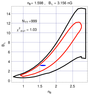
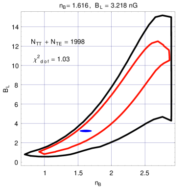
Figure 1: Likelihood contours in the plane $(n_{\mathrm{B}},\,B_{\mathrm{L}})$. In both plots the inner curve corresponds to $\Delta\chi^{2}=2.3$ (i.e. $68.3$% or $1\,\sigma$ of likelihood content) while the outer curve corresponds to $\Delta\chi^{2}=6.17$ (i.e. $95.4\,$% or $2\,\sigma$ of likelihood content).

In Fig. 1 the filled (ellipsoidal) spots in both plots highlight the minimal value of the $\chi^{2}$ (i.e. $\chi^{2}_{\mathrm{min}}$) while the contour plots represent the likelihood contours in the two parameters $n_{\mathrm{B}}$ and $B_{\mathrm{L}}$. In both plots of Fig. 1 the boundaries of the two regions contain $68.3\,$% and $95.4\,$% of likelihood as the values for which the $\chi^{2}$ has increased, respectively, by an amount $\Delta\chi^{2}=2.3$ and $\Delta\chi^{2}=6.17$. In the plot at the left of Fig. 1 the data points correspond to the measured TT correlations contemplating $N_{\mathrm{TT}}=999$ experimental points from $\ell=2$ to $\ell=1000$. In the plot at the right the data points include, both, the TT and TE correlations and the total number of data points increases to $N_{\mathrm{TT}}+N_{\mathrm{TE}}=1998$. The values of $n_{\mathrm{B}}$ and $B_{\mathrm{L}}$ minimizing the $\chi^{2}$ when only the TT correlations are considered turn out to be $n_{\mathrm{B}}=1.598$ and $B_{\mathrm{L}}=3.156\,\mathrm{nG}$ (see Fig. 1 plot at the left); in this case the reduced $\chi^{2}$ is $1.09$. When also the TE correlations are included in the analysis the reduced $\chi^{2}$ diminishes from $1.09$ to $1.03$ and the values of $n_{\mathrm{B}}$ and $B_{\mathrm{L}}$ minimizing the $\chi^{2}$ become $n_{\mathrm{B}}=1.616$ and $B_{\mathrm{L}}=3.218\,\mathrm{nG}$. In the frequentist approach, the boundaries of the confidence regions represent exclusion plots at $68.3\,$% and $95.4\,$% confidence level. In this sense the regions beyond the outer curves in Fig. 1 are excluded to $95$% confidence level.

In Fig. 2 the full line corresponds to the WMAP 5yr best fit of Eqs. (1)–(3). The (hardly distinguishable) dashed lines, in both plots, illustrate the m$\Lambda$CDM result for $(n_{\mathrm{B}}=1.616,\,B_{\mathrm{L}}=3.218\,\mathrm{nG})$ corresponding to $\chi^{2}_{\mathrm{min}}$, as determined from the joined analysis of the TT and TE angular power spectra (see plot at the right in Fig. 1). In both plots of Fig. 1 the (binned) data points are reported .

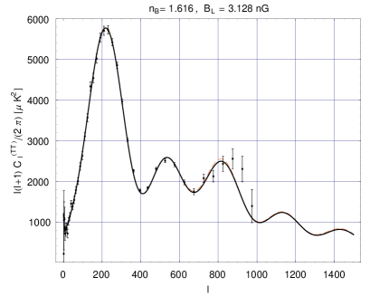
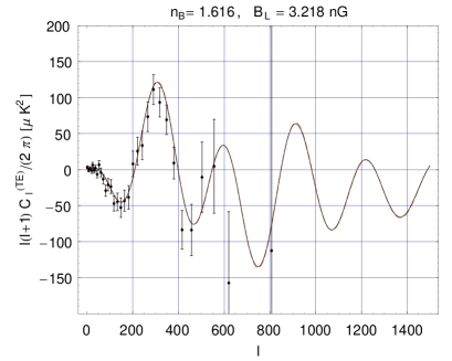
Figure 2: The TT and TE angular power spectra for the best-fit parameters stemming from the right plot of Fig. 1 (dashed line) and from the best fit to the WMAP 5yr data alone (full line). The data points of the WMAP 5yr release are included in their binned form.

The impact of the magnetic field parameters can be appreciated by monitoring the relative ratios of the first three peaks. Using the notation ${\mathcal{G}}_{\ell}=\ell(\ell+1)C_{\ell}/(2\pi)$, the relative heights of the acoustic peaks computed in the case of the best-fit of Fig. 2 are:

$$\overline{H}_{1}=\frac{{\mathcal{G}}_{\ell_{1}}}{{\mathcal{G}}_{\ell=10}}=6.942,\qquad\overline{H}_{2}=\frac{{\mathcal{G}}_{\ell_{2}}}{{\mathcal{G}}_{\ell_{1}}}=0.447,\qquad\overline{H}_{3}=\frac{{\mathcal{G}}_{\ell_{3}}}{{\mathcal{G}}_{\ell_{2}}}=0.981,$$ (11)

where $\ell_{1}=220$, $\ell_{2}=535$ and $\ell_{3}=816$ are, respectively, the locations of the first three acoustic peaks. In the the case of Eqs. (1)–(3) (i.e. in the absence of a magnetized background) the same ratios are, respectively, $\overline{H}_{1}=6.876$, $\overline{H}_{2}=0.447$ and $\overline{H}_{3}=0.963$. In Fig. 3 (plot at the left) the TT power spectra are illustrated with the same value of the spectral index as in Fig. 2 (i.e. $n_{\mathrm{B}}=1.616$) but with a magnetic field intensity $B_{\mathrm{L}}=6$ nG which is more than two $\sigma$ away from $\chi^{2}_{\mathrm{min}}$ (see Fig. 1, plot at the right): as expected, rough inspection of the left plot in Fig. 3, reveals that the m$\Lambda$CDM estimate does not correctly reproduce the data when ($n_{\mathrm{B}}=1.616$, $B_{\mathrm{L}}=6$ nG) especially around the first and third peaks. In the latter case the the relative ratios of the peaks become $(\overline{H}_{1},\overline{H}_{2},\overline{H}_{3})=(7.142,0.444,1.012)$: i.e. $\overline{H}_{1}$ and $\overline{H}_{3}$ exceed the best fit while $\overline{H}_{2}$ is comparatively lower than in Eq. (11). This is a general trend in the excluded region. Consequently, the whole approach of [9] is rather effective in constraining variations of $B_{\mathrm{L}}$ in the nG range. Similarly, by moving the magnetic spectral index in the excluded region of the parameter space the distortions of the peaks jeopardize the goodness of the fit.

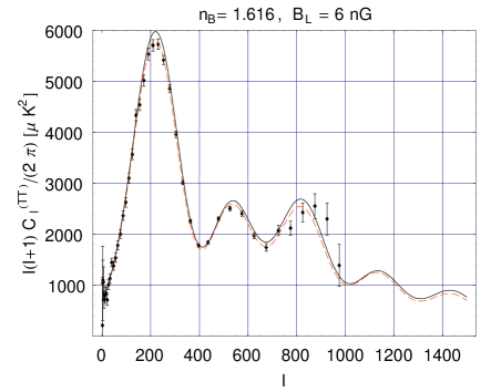
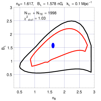
Figure 3: Left plot: the TT power spectra which are more than $2\sigma$ away from the best-fit point (full line) are compared with the best fit of Fig. 2 (dashed line). Right plot: contour plots in the $(n_{\mathrm{B}},B_{\mathrm{L}})$ plane for $k_{\mathrm{L}}=0.1\,\mathrm{Mpc}^{-1}$ (see also Fig. 1 where $k_{\mathrm{L}}=1\,\mathrm{Mpc}^{-1}$).

In Fig. 3 (plot at the right) the magnetic pivot wave-number has been moved from $k_{\mathrm{L}}=1\,\mathrm{Mpc}^{-1}$ to $k_{\mathrm{L}}=0.1\,\mathrm{Mpc}^{-1}$, consistently with the indetermination of the scale of protogalactic collapse. A reduction of the pivot wave-number implies that the magnetic field is regularized over a broader window in real space; hence the allowed amplitude of the putative magnetic field intensity is reduced. In the right plot of Fig. 3 the $\chi^{2}$ is minimized when $n_{\mathrm{B}}=1.617$ (i.e. comparable with the value of $n_{\mathrm{B}}$ deduced in Fig. 2 when $k_{\mathrm{L}}=1\,\mathrm{Mpc}^{-1}$) and, as anticipated, for a smaller magnetic field, i.e. $B_{\mathrm{L}}=1.578\,\mathrm{nG}$. The modification in the pivot wave-number also modifies the shape of the confidence contours (compare, e.g., Fig. 1 and Fig. 3).

The large-scale magnetic field possibly present prior to decoupling have been estimated, for the first time, from the temperature autocorrelations as well as from the cross-correlations between temperature and polarization in the case of the magnetized adiabatic mode [9]. The obtained results prove in explicit terms a guessed degeneracy between the spectral index and the magnetic field intensity. In a frequentistic perspective, beyond the outer contours of Figs. 1 and 3 the parameter space of the (minimal) m$\Lambda$CDM scenario is excluded to $95$% confidence level. Global observables (such as, for instance, the heights and depths of the acoustic oscillations) could be probably used as a normal parameter basis to infer an explicit analytic dependence of the TT and TE correlations upon the parameters of the magnetized background. In this direction work is in progress.

References

- [1] G. Hinshaw et al. [WMAP Collaboration], arXiv:0803.0732 [astro-ph].; J. Dunkley et al. [WMAP Collaboration], arXiv:0803.0586 [astro-ph]; E. Komatsu et al. [WMAP Collaboration], arXiv:0803.0547 [astro-ph].
- [2] D. N. Spergel et al. [WMAP Collaboration], Astrophys. J. Suppl. 170, 377 (2007); L. Page et al. [WMAP Collaboration], Astrophys. J. Suppl. 170, 335 (2007).
- [3] P. Astier et al. [The SNLS Collaboration], Astron. Astrophys. 447, 31 (2006); A. G. Riess et al. [Supernova Search Team Collaboration], Astrophys. J. 607, 665 (2004).
- [4] D. J. Eisenstein et al. [SDSS Collaboration], Astrophys. J. 633, 560 (2005).
- [5] R. Keskitalo, H. Kurki-Suonio, V. Muhonen and J. Valiviita, JCAP 0709, 008 (2007); J. Valiviita and V. Muhonen, Phys. Rev. Lett. 91, 131302 (2003); K. Enqvist, H. Kurki-Suonio and J. Valiviita, Phys. Rev. D 62, 103003 (2000).
- [6] R. Beck, Astron.Nachr. 327, 512 (2006).
- [7] C. Carilli and G. Taylor Ann. Rev. Astron. Astrophys. 40, 319 (2002).
- [8] Y. Xu, et al., Astrophys. J. 637, 19 (2006); M. Giovannini, Int. J. Mod. Phys. D 13, 391 (2004).
- [9] M. Giovannini, Phys. Rev. D 70, 123507 (2004); Phys. Rev. D 73, 101302 (2006); Phys. Rev. D 74, 063002 (2006); PMC Phys. A 1, 5 (2007); Phys. Rev. D 76, 103508 (2007); M. Giovannini and K. Kunze, Phys. Rev. D 78, 023010 (2008).
- [10] M. Giovannini, Phys. Rev. D 56, 3198 (1997); M. Giovannini and K. Kunze, Phys. Rev. D 77, 061301 (2008); ibid. 063003 (2008); arXiv:0812.2804 [astro-ph].
- [11] U. Seljak and M. Zaldarriaga, Astrophys. J. 469, 437 (1996); M. Zaldarriaga, D. N. Spergel and U. Seljak, Astrophys. J. 488, 1 (1997).
- [12] E. Bertschinger, COSMICS arXiv:astro-ph/9506070; C. P. Ma and E. Bertschinger, Astrophys. J. 455, 7 (1995).