The close Be star companion of $\mathrm{\beta}$ Cephei

Abstract

Context. The prototype of the $\mathrm{\beta}$ Cephei class of pulsating stars, $\mathrm{\beta}$ Cep, rotates relatively slowly, and yet displays episodic $\mathrm{H}\alpha$ emission. Such behaviour is typical of a rapidly rotating, classical Be star. For some time this posed a contradiction to our understanding of the Be phenomena as rapid rotation is thought to be a prerequisite for the characteristic emission phases of Be stars. Recent work has demonstrated that the $\mathrm{H}\alpha$ emission is in fact due to a close companion (separation $\mathrm{\approx}0.25\arcsec$) of the star. This resolves the apparent enigma if this close companion is indeed a classical Be star, as has been proposed.

Aims. We aim to test the hypothesis that this close companion is a valid Be star by determining properties such as its spectral type and $v\sin i$.

Methods. We employed the technique of spectroastrometry to investigate the close binary system. Using the spectroastrometric signatures observed, we split the composite binary spectra into its constituent spectra in the B band ($\mathrm{4}200-5000\AA$) and R band ($\mathrm{6}200-7000\AA$).

Results. The spectroastrometrically split spectra allow us to estimate spectral types of the binary components. We find that the primary of the close binary system has a spectral type of B2III and the secondary a spectral type of B5Ve. From the relationship between mass and spectral type, we determine the masses of the binary components to be $\mathrm{M}_{\mathrm{pri}}=12.6\pm 3.2M_{\sun}$ and $\mathrm{M}_{\mathrm{sec}}=4.4\pm 0.7M_{\sun}$ respectively. The spectroastrometric data allow some constraint on the orbit, and we suggest a moderate revision to the previously determined orbit. We confirm that the primary of the system is a slow rotator ($v\sin i$ = $\mathrm{2}9^{+43}_{-29}$ $\mathrm{km\,s^{-1}}$), while the secondary rotates significantly faster, at a $v\sin i$ = $\mathrm{2}30\pm 45$ $\mathrm{km\,s^{-1}}$.

Conclusions. We show that the close companion to the $\mathrm{\beta}$ Cephei primary is certainly a valid classical Be star. It has a spectral type of B5Ve and is a relatively fast rotator. We confirm that the $\mathrm{\beta}$ Cephei system does not contradict our current understanding of classical Be stars.

1 Introduction

The well-studied object $β$ Cephei is a massive, pulsating star with a spectral type of early B (Hoffleit & Warren 1995). The star is a prototype of a class of early B type giants and subgiants that exhibit rapid radial velocity, photometric and line profile variations due to pulsations (Sterken & Jerzykiewicz 1993). $\mathrm{\beta}$ Cep lies at a distance of $d\mathrm{=}182\pm 18$ pc and has a visual magnitude of 3.2 (Perryman & ESA 1997). Donati et al. (2001) estimate that the star has a bolometric magnitude of $L_{bol}=\mathrm{-}5.8\pm 0.2$ and a radius of $R_{*}=\mathrm{6}.5\pm 1.2$$\mathrm{R}_{\sun}$. Evolutionary tracks suggest that the star’s mass is $M_{*}\mathrm{=}12\pm 1$ $\mathrm{M}_{\sun}$ and that its age is approximately 12Myr (Donati et al. 2001). As such it seems to be a fairly typical $\mathrm{\beta}$ Cep star, as might be expected from the prototype of the class (Stankov & Handler 2005).

In fact, $\mathrm{\beta}$ Cep is a tertiary system. A visual companion lies at a distance of 13.4″from the primary (Heintz 1978). The primary also has a closer, spectroscopic companion at a separation of approximately 0.25″(Gezari et al. 1972). Hereafter, we refer to this star as the close companion and the primary of the system as $\mathrm{\beta}$ Cep. Little is known about the close companion. Measurements of the brightness difference between the primary and the close companion range from 5.0 magnitudes to 1.8 magnitudes (Gezari et al. 1972; Balega et al. 2002). Catanzaro (2008) indirectly estimated the $v\sin i$ of the close companion to be $\mathrm{\approx}230$ $\mathrm{km\,s^{-1}}$ and Pigulski & Boratyn (1992) estimated its mass to be $\mathrm{\approx}8M_{\sun}$. However, using the same orbital parameters but with a slightly reduced period Donati et al. (2001) conclude the secondary has a mass of $M_{*}=\mathrm{6}.2\pm 0.3M_{\sun}$.

H$\alpha$ emission emanating from $\beta$ Cep was first reported by Karpov (1932), and has since been found both absent and present with a recurring timescale of approximately a decade (Wilson & Seddon 1956; Kaper & Mathias 1995; Pan’ko & Tarasov 1997; Neiner et al. 2001). Such episodic emission is typical of a classical Be star. However, $\mathrm{\beta}$ Cep is a slow rotator with a rotational period of 12 days and a $v\sin i$ of approximately 25 $\mathrm{km\,s^{-1}}$ (Henrichs et al. 2000; Telting et al. 1997). Be stars are typically rapid rotators rotating at up to 80 % of their break-up velocity (Porter & Rivinius 2003). As this rapid rotation is thought to be integral to the H$\mathrm{\alpha}$ emission of Be stars, the H$\mathrm{\alpha}$ emission of $\mathrm{\beta}$ Cep is not consistent with the classical Be paradigm. Donati et al. (2001) proposed that the Be behaviour of the star is due to a magnetically confined wind leading to shocks in the equatorial region ($\mathrm{\beta}$ Cep does possess an oblique magnetic field). However, if this were the case, the $\mathrm{H}\alpha$ emission would be modulated by the rotation of the star, and it is not (Schnerr et al. 2006). Thus the source of the $\mathrm{H}\alpha$ emission has posed a conundrum to our current understanding of Be stars.

This enigma has been resolved by Schnerr et al. (2006), who used the technique of spectroastrometry to show the $\mathrm{H}\alpha$ emission is in fact due to the close companion to $\beta$ Cep. This companion may well be a classical Be star and if this is the case the contradictory nature of the system to current Be paradigms is negated. Schnerr et al. (2006) used spectra in the R band about H$\mathrm{\alpha}$. Here we use spectroastrometry to probe the blue region of the companion’s spectrum to test the hypothesis that the close companion is a classical Be star.

Spectroastrometry is a technique which utilises the spatial information present in a longslit spectrum. The information is contained in the spatial profile of the spectrum, specifically in the photocentre centroid and the spectral profile’s width. Changes in the flux distribution as a function of wavelength are manifest by changes in the centroid and width of the spectrum. An unresolved binary system with one star dominating the flux at an emission line is revealed by a centroidal displacement towards the dominating star over this line. Conversely, if one star of the system has a strong absorption line in its spectrum the centroid of the spectral profile will shift to the other star over this line. Such signatures can be detected with high precision, of the order of 1 mas or less (Oudmaijer et al. 2008). Therefore this is a powerful technique with which to detect and study close binary systems, as shown by Baines et al. (2006).

The spectroastrometric signature of an unresolved binary system contains information on the distribution of the flux emanating from the system. Thus spectroastrometry can be not only be used to detect binary systems, it can also deconvolve the observed spectrum into the individual spectra of its components. Here we use this technique to disentangle the spectra of the close $\mathrm{\beta}$ Cep binary components to investigate the properties of the close companion.

This paper is structured as follows: in Sect. 2 the details of the observations are presented, in Sect. 3 we present our spectroastrometric results, in Sect. 4 we discuss the spectra splitting methods and in Sect. 5 we present the results of splitting the spectra. A discussion and interpretation of the results follows in Sect. 6 and finally in Sect. 7 we summarise our findings.

2 Observations and data reduction

2.1 Observations

The data presented here were obtained using the 4.2m William Herschel Telescope (WHT) with the Intermediate Dispersion Spectrograph and Imaging System (ISIS) spectrograph. The data were obtained on the 7th of October 2006. Spectra of the $\mathrm{\beta}$ Cep system in the B ($\mathrm{4}200$-$\mathrm{5}000\AA$) and R ($\mathrm{6}200$-$\mathrm{6}900\AA$) bands were taken simultaneously using the dichoric slide of ISIS. The slit width was to set to 5″. The R1200 and B1200 gratings were used and the resolving power of the spectrograph was approximately 3800 (measured from telluric lines). The Marconi2 and EEV12 CCDs were used on the red and blue arm respectively, each with a pixel size of 13.5$\mathrm{\mu m}$. This resulted in angular pixel scales of 0.20″in the blue and 0.22″in the red region. As the average seeing during our observations was 1.27″the spectral profile was well sampled, which is a requirement for accurate spectroastrometry (Bailey 1998).

The data were gathered as part of wider study of binary systems. A wide slit ($\mathrm{5}^{\prime\prime}$) was used to ensure all the light from a given system entered the slit, despite the effect this had on the spectral resolution. Multiple spectra were taken at the following position angles (PA) on the sky: $\mathrm{0}^{\degr}$, $\mathrm{4}2^{\degr}$, $\mathrm{6}8^{\degr}$, $\mathrm{9}0^{\degr}$, $\mathrm{1}80^{\degr}$ and $\mathrm{2}70^{\degr}$. Data were taken at a PA of $\mathrm{4}2^{\degr}$ and $\mathrm{6}8^{\degr}$ as Schnerr et al. (2006) suggested the binary was orientated at $\mathrm{\approx}42^{\degr}$. Dispersion calibration arcs were made using CuNe and CuAr lamps.

2.2 Data reduction

Data reduction was conducted using the Image Reduction and Analysis Facility (IRAF) and routines written in Interactive Data Language (IDL). Flat field and bias frames were combined and the averaged flat field was then normalised. The raw data were then corrected using the averaged bias frame and the normalised average flat frame. Saturated exposures were discarded. The total intensity longslit spectra were then extracted from the corrected data in a standard fashion. Wavelength calibration was conducted using the arc spectra taken after the science observations at a position angle of $\mathrm{2}70^{\degr}$.

Spectroastrometry was performed by fitting Gaussian profiles to the spatial profile of the longslit spectra at each dispersion pixel. Spurious fits (for example due to cosmic rays) were identified and discarded, allowing the routine to fit the spectral profile. This resulted in a positional spectrum – the centroid of the Gaussian as a function of wavelength – and a FWHM (Full-Width-at-Half-Maximum) spectrum – the FWHM as a function of wavelength. The continuum position exhibited a general trend across the CCD chip (of the order of 10 pixels). This was removed by fitting a low order polynomial to the continuum regions of the spectrum. This set the continuum position of the centroid to zero. Spot checks were used to ensure line effects were not fit by the function.

A correction for slight changes in the dispersion was determined by cross correlating individual intensity spectra, and was then applied to the associated intensity, positional and FWHM spectra. This was to ensure slight changes in wavelength (due to flexure of the spectrograph) did not introduce spurious signatures when spectra obtained at differing position angles were combined. All intensity, positional and FWHM spectra at a given position angle were then combined to make an average spectrum for each position angle.

The average positional spectra for anti-parallel position angles were combined to form the average North-South (NS) and East-West (EW) positional spectra, i.e.: ($\mathrm{0}^{\degr}-180^{\degr}$)/2 and ($\mathrm{9}0^{\degr}-270^{\degr}$)/2. This procedure eliminates instrumental artifacts as real signatures rotate by $\mathrm{1}80^{\degr}$ when viewed at the anti-parallel position angle while artifacts remain at a constant orientation. However, in some of the data a signature was noted at only one position angle. Subtraction of the two anti-parallel spectra would not remove this effect but clearly it is also an artifact. Thus all average position spectra were assessed visually to exclude features only present at a single position angle. Signatures in data taken at position angles with no anti-parallel counterpart were judged real if they exhibited qualitative similarity to signatures at a similar position angle that were judged real. The FWHM spectra at opposite position angles were visually inspected to search for artifacts. Features present in data taken at only one position angle were classified as an artifact and discarded. FWHM spectra at anti-parallel position angles were combined to make an average NS or EW FWHM spectrum.

3 Results: The spectroastrometric signatures observed

3.1 The spectrum of $\mathrm{\beta}$ Cep

In Fig. 1 we present the average spectra observed in both the B and R range. H$\mathrm{\alpha}$ can be seen in absorption with a small double peaked emission profile, with the blue peak just rising above the continuum level. The hydrogen Balmer line profiles are also presented in the top panels of Fig. 2. No emission is noticeable in the H$\mathrm{\beta}$ and H$\mathrm{\gamma}$ lines. Besides $\mathrm{H}\alpha$ other prominent lines in the red region are He i at $\mathrm{6}678\AA$ and a Diffuse Interstellar Band (DIB) at $\mathrm{\approx}6280\AA$. In the blue region many more absorption lines are present, most prominent of which are the lines due to H i and He i. The numerous weaker and narrow lines present are primarily due to O ii, Si ii, Si iii and other ionised metals such as C ii and N ii.

Figure 1: The average spectra of $\mathrm{\beta}$ Cep (total light of the binary system) in the blue (upper panel) and the red (up to the telluric lines – lower panel) spectral range.

3.2 The spectroastrometric results

The spectroastrometric signatures of the close $\mathrm{\beta}$ Cep binary system over the three principle hydrogen Balmer lines are presented in Fig. 2. For each line we present: the intensity profile and the centroidal signature and change in the FWHM of the longslit spectra over these lines in the NS and EW directions. The photocentre of the spectral profile shifts to the North and East and the FWHM increases over these lines. This means we clearly detect the close binary system – something not trivial in seeing conditions of greater than 1″. The signature is most prominent over the $\mathrm{H}\alpha$ line while small and consistent features can be noted across H$\mathrm{\beta}$ and $\mathrm{H}\gamma$. The spectroastrometric signature observed over the emission component of the H$\mathrm{\alpha}$ profile implies that the source of the emission lies to the North-East (NE) and the emission profile is intrinsically broader than the absorption profile. This confirms the result of Schnerr et al. (2006), i.e. the H$\mathrm{\alpha}$ emission is emanating from the companion in the NE and not the primary.

Across the $\mathrm{H}\beta$ and H$\mathrm{\gamma}$ lines the positional excursions occur in the same direction as over H$\mathrm{\alpha}$. As these signatures take place across an absorption line this indicates that the South-West (SW) component of the system ’dominates’ the absorption profile. In addition narrow positional excursions to the NE and FWHM increases can be seen over the lines seen alongside H$\mathrm{\gamma}$ (primarily O ii lines). This indicates that these lines are associated with the SW component of the system, the primary. These data highlight the exquisite sensitivity of spectroastrometry to changes in the flux distribution. Changes in the photocentre of the order of 5 mas or less are detected. The noise in the positional spectra is typically of the order of 1 mas.

The ’XY plots’ (NS against EW excursions) of the $\mathrm{\beta}$ Cep system are presented in Fig. 3. The XY plots trace a straight line to the North and East – the direction in which the source of the H$\mathrm{\alpha}$ emission lies. The position angle of the binary is determined from a simple least-squares fit to the data, and is in general consistent across the different lines ($\mathrm{H}\alpha$: $\mathrm{5}1.3\pm 0.7\degr$, $\mathrm{H}\beta$: $\mathrm{6}6.5\pm 4.6\degr$ & $\mathrm{H}\gamma$: $\mathrm{5}8.7\pm 6.7\degr$). However, the H$\mathrm{\beta}$ position angle is not consistent with the H$\mathrm{\alpha}$ data. The H$\mathrm{\beta}$ and H$\mathrm{\gamma}$ lines were associated with much weaker positional excursions and as such these position angles are more uncertain than the position angle derived from the H$\mathrm{\alpha}$ data.

Figure 2: The spectroastrometric signature of the close $\mathrm{\beta}$ Cep binary system across the $\mathrm{H}\alpha$, H$\mathrm{\beta}$ and H$\mathrm{\gamma}$ lines (from left to right). Across each line we present the averaged intensity profile normalised to the continuum, the position of the photocentre with respect to the continuum position in the NS and EW direction and the FWHM of the spectral spatial profile, with respect to the continuum value, in the same directions. In the positional spectra North and East are presented as being in the positive direction (i.e. to the top of the page).

Figure 3: XY plots of the spectroastrometric signature of the close $\mathrm{\beta}$ Cep binary system over the H$\mathrm{\alpha}$, H$\mathrm{\beta}$ and H$\mathrm{\gamma}$ lines. The solid line is a fit to the H$\mathrm{\alpha}$ data, the dotted line is a fit to the H$\mathrm{\beta}$ data and the dashed line a fit to the H$\mathrm{\gamma}$ data. North is to the top of the page and East is to the left.

4 Splitting the spectra

Two approaches were used to split entangled/composite binary spectra. The first approach was pioneered by Bailey (1998). This method utilises the fact that the changes in the flux ratio of a binary system lead to positional displacements of the photocentre. The movement of the photocentre across a given wavelength is proportional to the component separation and the component flux ratio at the particular wavelength. This centroid movement takes place about the continuum position, which is determined by the continuum brightness ratio of the two components. Therefore if the separation and the continuum flux ratio of the two components are known the intensity spectra and positional spectra observed can used to disentangle the individual fluxes of the two components.

The second approach, that of Porter et al. (2004), does not require any prior knowledge of the binary system. This method not only deconvolves spectra, it also estimates the separation of the two binary components. This method is based upon numerical simulations of point source binary systems performed by Porter et al. (2004). Porter et al. (2004) determined the dependence of the spectroastrometric signature of a given binary on the system’s properties. Using the relationships established by these simulations one can use the three spectroastrometric observables (the centroid, total flux and width at a given $\mathrm{\lambda}$), with knowledge of the seeing, to recover the individual fluxes of the binary components. For a full description of the method see Porter et al. (2004).

We have used both methods for two reasons. Firstly there are certain limitations to the method of Porter et al. (2004). We found accurate knowledge of the seeing was essential, something not trivial in this case. To test the reliability of the method of Porter et al. (2004) we applied this method on simulated data. It was found that with accurate knowledge of the seeing this method consistently returned the separation of the two point sources and their respective fluxes, to within an error of $\mathrm{\approx}10\%$ or better. However, when adopting the minimum FWHM as an estimate of the seeing (which is actually an upper limit) the method can under estimate the separation. While we expect this effect to be small we treat our estimate of $\mathrm{\sigma}_{s}$ with caution and use the method of Bailey (1998) as a consistency check.

Secondly, we do not just use the method of Bailey (1998) as although we can find literature values for the difference in brightness of the two components and their separation, none are certain. The difference in magnitude reported ranges from 1.8 to 5.0 (Balega et al. 2002; Gezari et al. 1972) while the separation changes slowly due to the motion of the binary system. The orbit has been determined by Pigulski & Boratyn (1992). However this orbit is not consistent with our results and those of Schnerr et al. (2006) (see Sect. 6.2). Therefore, we do not use the orbital parameters of Pigulski & Boratyn (1992) to estimate the position of the secondary. Thus we used each method as a consistency check upon the other.

4.1 The method of Bailey (1998)

The method of Bailey (1998) uses two spectroastrometric observables (centroidal excursions and the total flux observed) and two inputs (binary projected separation and difference in brightness). Three values for the difference in brightness between the binary components were taken from the literature: 1.82 magnitudes at $\mathrm{\lambda}\approx 8100\AA$, a rough average value of 3.4 magnitudes around $\mathrm{5}500\AA$ and 5 magnitudes at $\mathrm{5}000\AA$ (Balega et al. 2002; Hartkopf et al. 2001; Gezari et al. 1972). Distances in the literature between the primary and the secondary range from $\mathrm{\approx}0.25\arcsec$ to 0.04″. The most recent observation of the system was in 1998, and thus the position of the secondary in 2006 is uncertain.

We used a range of distances (0.05″to 0.25″) with each of the magnitude differences listed above, and evaluated the results based on the following criteria. Any input parameters leading to negative flux in the secondary spectra were immediately disregarded. Also situations where absorption lines in the primary were mirrored by an emission line in the secondary spectra were considered unlikely.

In the red region a brightness difference of 5 magnitudes was discarded as it resulted in secondary spectra with negative flux. A difference in brightness of 3.4 magnitudes was discounted as this led to secondary spectra with He i $6678\AA$ in emission, an uncommon occurrence in field stars. Using $\Delta R$ of 1.8 with a range of separations did not result in a significant constraint upon the separation of the two components. A separation of 0.05″was discarded as this resulted in He i emission in the secondary spectrum. Separations of 0.1″to 0.15″resulted in a secondary spectrum devoid of any He i $\mathrm{6}678\AA$ feature while separations of 0.20″and 0.25″led to a secondary spectra with a He i $\mathrm{6}678\AA$ absorption feature. If the secondary is a mid B type star the presence of He i 6678$\rm\AA$ is to be expected, but the absence of a He i feature is consistent with a late type B star. Both spectral types are possible and thus the binary separation is not constrained beyond the range 0.05″and 0.25″.

In Fig. 4 we present the average red spectra of the close $\mathrm{\beta}$ Cep binary system, split using the method of Bailey (1998), a brightness difference of 1.8 magnitudes and separations of $\mathrm{0}.05^{\prime\prime}$, $\mathrm{0}.15^{\prime\prime}$ and $\mathrm{0}.25^{\prime\prime}$. It is evident that the H$\mathrm{\alpha}$ emission is associated with the secondary. The double peaked H$\mathrm{\alpha}$ emission profile is typical of rapidly rotating classical Be stars.

Figure 4: The red spectrum of the close $\mathrm{\beta}$ Cep binary system, split using the method Bailey (1998), $\mathrm{\Delta}R$ of 1.8 and a range of binary separations: 0.05″(long-dashed line), 0.15″(short-dashed line) and 0.25″(solid line). In the top left the wavelength range is reduced and centred on $\mathrm{H}\alpha$ while in the top right attention is focused upon the He i $\mathrm{6}678.15\AA$ profile.

When splitting the blue spectra differences in brightness between the two binary components of 5.0 and 3.4 were discarded due to similar arguments as presented above. Thus it appears the brightness difference between the two binary components in the B band is approximately 1.8 magnitudes, as in the R band. In Fig. 5 we present the spectra obtained with this value of $\mathrm{\Delta}$B and a separation of 0.20″. The many narrow absorption lines present in the composite spectrum (O ii, Si iii etc.) are clearly associated with the primary spectrum. Also evident is that the He i absorption lines are weaker in the secondary spectrum than in the primary spectrum. The secondary spectra obtained using smaller separations were judged to be of dubious validity as they exhibited many emission features coincident with absorption features in the primary spectrum.

Figure 5: The blue spectrum of the close $\mathrm{\beta}$ Cep binary system, split using the method Bailey (1998), $\mathrm{\Delta}$ B = 1.8 and d = 0.20$\mathrm{{}^{\prime}}^{\prime}$. In the top left the wavelength range is reduced and centred on $\mathrm{H}\gamma$ while in the top right attention is focused upon the H$\mathrm{\beta}$ profile.

4.2 The method of Porter et al (2004)

The model of Porter et al. (2004) is based on a constant convolving function, yet a change in focus along the chip length led to a change in the width of the flux distribution. To negate this difficulty the $\mathrm{\sigma}$ distribution was normalised via a polynomial fit to remove changes not due to the binary system. The mean seeing was estimated from the minimum of the now flattened FWHM spectrum. However, this estimate of the seeing is an upper estimate. Simulating a binary system with a separation of 0.20″and a difference in brightness of 1.8 magnitudes we found the minimum FWHM may over estimate the seeing by 0.02 pixels. Thus we subtracted this from our estimate of the seeing using the FWHM minimum.

In figure 6 we present the red spectrum of the $\mathrm{\beta}$ Cep system split using the method of Porter et al. (2004). The spectrum exhibits a close similarity to the spectrum obtained using the method of Bailey (1998) and similar parameters as those output by the method of Porter et al. (2004).

Figure 6: The red spectrum of the close $\mathrm{\beta}$ Cep binary system, split using the method Porter et al. (2004). In the top left the wavelength range is reduced and centred on $\mathrm{H}\alpha$ while in the top right attention is focused upon the He i $\mathrm{6}678.15\AA$ profile. The determined values for the separation and brightness difference were $d\mathrm{=}0.21\pm 0.07\arcsec$ and $\Delta R\mathrm{=}1.5\pm 0.17$

Applying the method of Porter et al. (2004) to the blue spectra did not result in separated spectra, as the model did not converge upon the most likely separation. This could be due to a lack of prominent features in the position spectra. The precision of the blue position spectra was no worse than that in the red spectra (of the order of 1 mas). However, the positional offsets in the blue region are much smaller than in those in the red region as the flux difference in the blue region is less pronounced than that over the H$\rm\alpha$ line.

5 Results: the separated spectra

5.1 The spectral types of the binary components

The spectral type of $\mathrm{\beta}$ Cep has been estimated to be both B1 and B2 while the luminosity class of the star has been reported to be III, IV and V (Morgan et al. 1943, 1955; Lesh 1968; Morel et al. 2006). These spectral classifications refer to the total light of the system. As we have disentangled the spectra of the binary components we can now spectrally type each component separately. The spectrum of the binary system has also been designated ’e & v’ where e refers to the emission nature and v the variability of the spectrum. We assume the that the primary is responsible for the variability of the spectrum due to its pulsating nature. To determine the spectral type of the binary components we use the spectra that were separated with the method of Bailey (1998), a brightness difference of 1.8 magnitudes and a separation of 0.2$\mathrm{{}^{\prime}}^{\prime}$.

The presence of He i absorption in the red spectrum of the primary indicates a B type star. The equivalent widths of the H$\mathrm{\alpha}$ and He i absorption features suggest that the primary is an early B (1-3) type star, with a luminosity class of IV or III. In the blue region the primary spectrum exhibits prominent H i absorption lines ($\mathrm{H}\beta$ and $\mathrm{H}\gamma$) alongside He i absorption lines, which indicates a B type star. The relatively strong He i lines and comparatively weak H i lines indicate that the primary is an early B type star (i.e. B0 to B2). Additional features in the primary spectrum include absorption lines due to He i, O ii, Si iii, C ii, C iii and N ii, lines which are also suggestive of an early B type star. No He ii lines are present, implying the star has a spectral type later than O9. The ratio of the He i 4471 $\mathrm{\AA}$/Mg ii 4481 $\mathrm{\AA}$ lines indicate the star is an early B type star, most probably B2. To determine the luminosity class of the star the ratios of the O ii 4415$\mathrm{\AA}$ & 4417$\mathrm{\AA}$ to He i 4387$\mathrm{\AA}$ and O ii 4348$\mathrm{\AA}$ to H$\mathrm{\gamma}$ lines were used. The strength of the O ii lines indicates that the primary’s luminosity class is most probably III.

To summarise, the spectral type of the primary was determined to be B2III. The uncertainty associated with this conclusion is approximately one spectral subtype.

The most prominent feature in the red spectrum of the secondary is that of the H$\mathrm{\alpha}$ emission. The H$\mathrm{\alpha}$ emission extends approximately $\mathrm{\pm}400$ $\mathrm{km\,s^{-1}}$ from the rest wavelength of H$\mathrm{\alpha}$, as also found by Schnerr et al. (2006). A Gaussian fit to the $\mathrm{H}\alpha$ emission profile results in a value for the FWHM of the profile of $\mathrm{\approx}$ $\mathrm{500km\,s^{-1}}$. This width is typical of a rapidly rotating Be star. A He i $\mathrm{6}678\AA$ absorption feature is present, although weak, with an equivalent width of $\mathrm{\mathrm{missing}}\approx 0.25\AA$. This places an upper limit on the spectral type of about B4/B5.

The secondary spectrum in the blue does not display the many narrow absorption features due to O ii and Si iii the primary does. Thus there is no reason to suspect it is not a dwarf star. The spectrum of the secondary in the blue region exhibits absorption lines due to H i ($\mathrm{H}\beta$ and $\mathrm{H}\gamma$) and He i (i.e. $\mathrm{4}388,4471\AA$). This is indicative of a B type star. The He i lines are weaker than than those in the spectrum of the primary (equivalent widths are approximately 15% less) which suggests the secondary is of a later spectral type than the primary. This is to be expected as it is less bright. In contrast, the H i lines in the secondary are of a similar strength to those in the primary, indicating an early B type star. However, as the secondary shows emission in H$\mathrm{\alpha}$ it is possible there is some emission in H$\mathrm{\beta}$ and H$\mathrm{\gamma}$ which ’fills in’ the absorption profile of the secondary. Concentrating on the strength of the He i lines, and the ratio of He i/Mg ii (4471/4481$\mathrm{\AA}$) lines, we conclude the most likely spectral type of the secondary is B5.

Therefore the spectral type of the secondary is determined to be B5Ve. The uncertainty in this spectral typing is again approximately one spectral subtype.

In determining the spectral type of the secondary we assume that all the flux observed emanates directly from the star in question and the spectral features observed are purely photospheric in their origin. To asses the possible flux contribution from circumstellar material we use the NIR study of Dougherty et al. (1991). In most cases mid type Be stars were found to have a small V-J excess, the average (V-J) excess of a B5Ve star according to Dougherty et al. (1991) is only $\sim$6% of the stellar continuum. In addition the continuum excess falls off very sharply with decreasing wavelengths. Therefore we expect the continuum excess due to any circumstellar material to be negligible at optical wavelengths. Regarding emission lines there may well be unresolved H i lines in the secondary spectrum therefore we do not rely on the strength of the H i lines to determine the spectral type of the secondary. There may also be some emission component in the He i lines. However, in a study of more than 100 Be stars over a period of 10 years Chauville et al. (2001) did not observe any Be star with net He i 4471$\rm\AA$ emission. Therefore, in light of the above comments, we assume that the He i lines observed are photospheric in origin.

5.2 The mass ratio of the close binary system

Taking the spectral type of the primary to be B2III and that of the secondary to be B5V and using the tabulated values of Landolt et al. (1982) and Harmanec (1988) we obtain values for the masses of the components of the system of $M_{\mathrm{pri}}\mathrm{=}12.6\pm 3.2M_{\sun}$ and $M_{\mathrm{sec}}\mathrm{=}4.4\pm 0.7M_{\sun}$ respectively. Uncertainties were estimated by allowing an uncertainty in the spectral types of one subtype. The mass ratio of the system is determined to be $\mathrm{0}.35\pm 0.15$.

5.3 The $v\sin i$ of the individual binary components

Using the separated spectra the $v\sin i$ values of each component of the binary system can be estimated. A rotational profile was constructed for a variety of $v\sin i$ values: from 1 to 550 $\mathrm{km\,s^{-1}}$ in steps of 1 $\mathrm{km\,s^{-1}}$. The rotation profile was then convolved with synthetic spectra constructed using ATLAS9 and SYNTHE (Kurucz 1993). Following the convolution of the rotational profile and the synthetic spectra the resultant spectra were broadened by convolution with a Gaussian function to match the spectral resolution. The rotationally broadened profile of the He i 4471 $\mathrm{\AA}$ line was then compared with the observed profile using a simple $\mathrm{\chi}^{2}$ test.

For the primary synthetic spectra were constructed using values of $T_{\mathrm{eff}}$ of 23000K, 24000K and 25000K and $\log(g)$ of 3.8. These values were based on the values determined by Catanzaro (2008) and the spectral type determined previously. To simulate the spectrum of the secondary synthetic spectra were constructed using values of $T_{\mathrm{eff}}$ of 14000K, 15000K, 16000K and 17000K and $\log(g)$ of 4.1. These values are based on a B5 type dwarf star on the Main Sequence (Harmanec 1988). The range of temperatures used reflects the uncertainty in the spectral typing. A micro-turbulence of $\mathrm{2}$ $\mathrm{km\,s^{-1}}$ was used in the synthetic spectra generation, and when constructing the rotational profiles a limb-darkening coefficient of 0.6 was assumed.

Figure 7: A comparison between the spectroastrometrically separated He i 4471$\mathrm{\AA}$ profiles and the best fit rotationally broadened synthetic profiles. The solid line represents the He i line of the primary and secondary spectra respectively, the short-long dashed line the best fit primary synthetic spectrum ($T_{\mathrm{eff}}$ 24000K, $\log(g)$ 3.8, $v\sin i$ 29 $\mathrm{km\,s^{-1}}$), the short-dashed line the best fit secondary synthetic spectrum at a $T_{\mathrm{eff}}$ of 15000 K ($\log(g)$ 4.1, $v\sin i$ $\mathrm{1}63$ $\mathrm{km\,s^{-1}}$) and the long dashed line is the best fit secondary synthetic spectrum at a $T_{\mathrm{eff}}$ of 17000 K ($\log(g)$ 4.1, $v\sin i$ $\mathrm{2}30$ $\mathrm{km\,s^{-1}}$).

The best fit $v\sin i$ values obtained are dependent upon the value of $T_{\mathrm{eff}}$ used to generate the synthetic spectrum. This is because the depth of the He I line increases towards earlier types. With the previous spectral typing an error in $T_{\mathrm{eff}}$ of $\mathrm{\approx}1000$K possible. However, the input $T_{\mathrm{eff}}$ does not effect the width of the convolved profile. Thus the most likely value of $T_{\mathrm{eff}}$ is the one for which the rotationally broadened synthetic spectrum matches not only the height but also the width of the observed profile at a given value of $v\sin i$ (i.e. that associated with the smallest $\mathrm{\chi}^{2}$). This effect is illustrated in Fig. 7 by plotting the best fit rotationally broadened profiles at 15000K and 17000K over the secondary profile. The best fit at 15000K fails to fit the width and depth of the observed profile, which was reflected in the large value for the minimum $\mathrm{\chi}^{2}$ at this temperature. The best fit $v\sin i$ values were lower for lower values of $T_{\mathrm{eff}}$ and ranged from $v\sin i\mathrm{=}132$ $\mathrm{k}m\,s^{-1}$ at $T_{\mathrm{eff}}$ of 14000K to $v\sin i\mathrm{=}230$ $\mathrm{k}m\,s^{-1}$ at $T_{\mathrm{eff}}$ of 17000K. The lowest $\mathrm{\chi}^{2}$ values were obtained with a $T_{\mathrm{eff}}$ of 24000K in the case of the primary and 17000K in the case of the secondary. We determine that the primary has a $v\sin i$ of $\mathrm{2}9^{+43}_{-29}$ $\mathrm{km\,s^{-1}}$ and the secondary has a $v\sin i$ of $\mathrm{2}30\pm 45$ $\mathrm{km\,s^{-1}}$. The uncertainties in these values were determined from the change in $v\sin i$ of the synthetic spectra which led to an increase in the $\chi^{2}$ of the fit of 1. We note that the secondary profile was best fit using a B4 star profile ($T_{\mathrm{eff}}$ = 17000K), rather than a B5 profile. This is consistent with an uncertainty of 1 subtype in the spectral type of the secondary.

6 Discussion

6.1 The $v\sin i$ of the individual binary components

The $v\sin i$ of the primary is consistent with literature values of around 25 $\mathrm{km\,s^{-1}}$ (Telting et al. 1997), although it is imprecise. This imprecision is due to the use of a relatively wide slit resulting in an instrumental profile with a FWHM of $\mathrm{\approx}70$ $\mathrm{km\,s^{-1}}$. The $v\sin i$ value for the secondary is similarly imprecise. However, it is clear that the secondary does rotate substantially faster than the primary, in agreement with the estimate of $\mathrm{\approx}230$ $\mathrm{km\,s^{-1}}$ of Catanzaro (2008).

Given the spectral type of the secondary it’s critical velocity is approximately $\mathrm{\approx}430$ $\mathrm{km\,s^{-1}}$ (Townsend et al. 2004). It is suggested that the orbit of the $\mathrm{\beta}$ Cep system is seen almost edge on (Pigulski & Boratyn 1992, see also Sect. 6.2). If the stars rotate in the plane of the orbit, which is not necessarily the case, then the above $v\sin i$ values are the intrinsic rotation velocities of the stars. In this case the rotational velocity of the secondary is 45-65% of its critical velocity. This rotation may not be consistent with the hypothesis that the secondary is a classical Be star.

Whether or not all Be stars rotate at their break-up velocity is currently a matter or some debate, with arguments both for (Townsend et al. 2004) and against (Cranmer 2005) this scenario. However, it is generally accepted that all Be stars rotate at a substantial fraction of their break-up velocity. To prove the secondary is rotating at/near its critical velocity we need an independent determination of its inclination, which is far from trivial. In addition even if $i$ was constrained, this $v\sin i$ measurement would not be conclusive. It has been shown the method used here to determine $v\sin i$ returns a lower limit as it does not account for gravity darkening (Townsend et al. 2004). However, the secondary is shown to be rotating relatively fast, even at the lower limit of $i$ = 90^∘, and it may be rotating at a substantial fraction of its break-up velocity. This is essentially consistent with the finding of Porter (1996) who demonstrated Be stars intrinsically rotate at approximately 70% of their break-up velocity (using a similar technique to estimate $v\sin i$). Therefore it is indeed likely the secondary is a classical Be star.

6.2 The orbit of $\mathrm{\beta}$ Cephei

The orbit of the close companion to $\mathrm{\beta}$ Cep has been determined by Pigulski & Boratyn (1992). However, both the results presented here and by Schnerr et al. (2006) suggest a revision of the orbital parameters is required. According to the orbit of Pigulski & Boratyn (1992) the companion to $\mathrm{\beta}$ Cep should have been to the SW of the primary in 2006. The data presented here, and by Schnerr et al. (2006) are not consistent with this prediction. As the spectroastrometric data proves the H$\mathrm{\alpha}$ emission is emanating from the close companion, the data place the companion to the NE of the primary in 2006.

Here we investigate whether a slight change of orbital parameters can result in an orbit consistent with observations. It was found the data allow a straight line fit, which implies that the system is viewed at a very high inclination, i.e. $\mathrm{\approx}90^{\degr}$. From a least-squared fit to the data we obtain a value for the position angle of the line of nodes to be $\mathrm{2}28.6\pm 1.4^{\degr}$. We took the date of 1914.6 as our reference periastron, as did Pigulski & Boratyn (1992). For the period of the orbit we considered the suggestion of Hadrava & Harmanec (1996) that the system was approaching periastron in 1996. This period of 81.4 years differs from the value used by Pigulski & Boratyn (1992) but is within $\mathrm{3}\sigma$ of their value. The semi-major axis of the orbit was estimated via Kepler’s third law, the above period and the total mass of the system. With the data at our disposal constraining e and $\mathrm{\omega}$ is difficult. We set e at 0.6 and investigated what value of $\mathrm{\omega}$ was required to fit the observational data, given the parameters determined above. We found a value of $\mathrm{\omega}$ of $\mathrm{2}0.0^{\degr}$ fit the data well (see Fig. 8).

The final orbital parameters used were: $\mathrm{P}_{orb}=81.4yr$, $\mathrm{e}=0.60$, $\mathrm{T}_{0}=1914.6$, $\mathrm{\Omega}=228.6^{\degr}$, $\mathrm{i}=90.0^{\degr}$, $\mathrm{a}=0.25^{\prime\prime}$ and $\omega=20^{\degr}$. Most parameters are within 3$\mathrm{\sigma}$ of the values of (Pigulski & Boratyn 1992). The orbit is consistent with previous speckle interferometric observations of the system and our spectroastrometrically determined position of the secondary. Admittedly, systems are rarely observed at an inclination of exactly $\mathrm{9}0^{\degr}$. Changing the inclination by up to a few degrees does little to qualitatively change the picture. Provided $\mathrm{\Omega}$ is revised in light of any inclination changes, a consistent fit to the data is achieved when $i$ is changed by a few degrees (see Fig 8). We stress such an orbit is only illustrative, and more observations are needed to fully constrain all the orbital parameters. However, we successfully demonstrate a slight revision of the orbital parameters of Pigulski & Boratyn (1992) is all that is required to obtain an orbit consistent with observations.

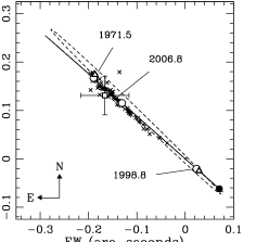
Figure 8: A possible relative orbit of the companion of the close $\mathrm{\beta}$ Ceph system about the primary. Speckle interferometric data have been taken from Pigulski & Boratyn (1992) and Hartkopf et al. (2001), and are marked by crosses. The open square point represents the position of the companion from our spectroastrometric data, the line indicates the orbital path. We compare specific orbital predictions and data points at three epochs, 1971.5, 1998.8 and 2006.8. We denote these data points by open triangles (a square in the case of 2006.8) and orbital predictions by open circles. The primary is situated at 0,0 and the filled circle marks the position of periastron. The dashed line shows the orbital path when $i$ is changed by $\mathrm{-}2^{\degr}$ and $\mathrm{\Omega}$ is changed by $\mathrm{-}3^{\degr}$. The average uncertainty in the data was approximately 0.015$\mathrm{{}^{\prime}}^{\prime}$ in each direction.

7 Conclusions

In this paper we have studied the close binary system of $\mathrm{\beta}$ Cep utilising the novel approach of splitting the binary spectra using spectroastrometry. Disentangling the composite binary spectrum allows us to determine key properties of each component. We find that the $\mathrm{H}\alpha$ emission of the system is due to the close secondary, as shown by Schnerr et al. (2006). Splitting the convolved spectrum and assessing the spectral type of each component we find that the companion is a dwarf star with a spectral type of B5. We also find it may rotate at a substantial fraction of its critical velocity, with a lower limit of $v\sin i$ = 230 $\mathrm{km\,s^{-1}}$ corresponding to $V_{\mathrm{r}}/V_{\mathrm{crit}}$ of 53%.

The secondary’s estimated mass and $v\sin i$ fall within the range of typical values for classical Be stars. Thus we consider it highly likely the secondary is indeed such a star. Therefore we have not only confirmed the result of Schnerr et al. (2006) but we validate their suggestion that the secondary could be a classical Be star. In which case the H$\mathrm{\alpha}$ emission is thought to be due to gaseous equatorial material ejected from the star by a combination of rapid rotation and some other phenomena, e.g. non-radial pulsation (Porter & Rivinius 2003). As the H$\mathrm{\alpha}$ emission is shown to originate from a star where the standard Be paradigm applies the $\mathrm{\beta}$ Cep system does not pose any contradictions to the current understanding of either $\mathrm{\beta}$ Cep stars or classical Be stars.