Efficient pseudo-global fitting for helioseismic data

Abstract

Mode fitting or “peak-bagging” is an important procedure in helioseismology allowing one to determine the various mode parameters of solar oscillations. Here we describe a way of reducing the systematic bias in the fits of certain mode parameters that are seen when using “local” fitting techniques to analyse the sun-as-a-star p-mode power spectrum. To do this we have developed a new “pseudo-global” fitting algorithm designed to gain the advantages of fitting the entire power spectrum, but without the problems involved in fitting a model incorporating many hundreds of parameters.

We have performed a comparative analysis between the local and pseudo-global peak-bagging techniques by fitting the “limit” profiles of simulated helioseismic data. Results show that for asymmetric modes the traditional fitting technique returns systematically biased estimates of the central frequency parameter. This bias is significantly reduced when employing the pseudo-global routine. Similarly, we show that estimates of the background returned from the pseudo-global routine match the input values much more closely than the estimates from the local fitting method.

We have also used the two fitting techniques to analyse a set of real solar data collected by the Global Oscillations at Low Frequencies (GOLF) instrument on board the ESA/NASA Solar and Heliospheric Observatory (SOHO) spacecraft. Similar differences between the estimated frequencies returned by the two techniques are seen when fitting both the real and simulated data. We show that the background fits returned by the pseudo-global routine more closely match the estimate of the background one can infer from interpolating between fits to the high and low frequency ends of the p-mode power spectrum.

1 Introduction

Determining the parameter values of the resonant modes of oscillation of the Sun is an important process in helioseismology. Mode frequencies, rotational splittings, lifetimes and amplitudes can all be used to help identify the conditions of the solar interior. For example, by employing inversion techniques the mode frequencies can be used to constrain estimates of the sound speed and density in the solar interior, while the rotational splitting parameter can determine the internal rotation rate. The mode linewidths and amplitudes may be used in order to better understand possible models of convection within the outer layers of the solar interior.

Over the years the quality of helioseismic data has improved significantly due to the length of data sets increasing, signal-to-noise ratios being improved and more continuous observations being made, both from ground-based networks and space-borne missions. This has led to the parameter values being constrained with increasingly greater precision which in turn has led to better constraints on our understating of the solar interior.

As the precision of the parameter estimates increases so more subtle characteristics of the p-mode power spectrum are being uncovered. An example of this is the discovery that the resonant mode peaks that make up the p-mode spectrum are actually slightly asymmetric (e.g., Duvall et al. 1993; Chaplin et al. 1999). This supported prior theoretical predictions (e.g., Gabriel 1992, 1995b) and added to the evidence that acoustic waves are generated within a well-localized region of the solar interior and are possibly correlated with the background generated by solar granulation (Nigam & Kosovichev, 1998; Toutain et al., 2006).

In order to analyse such subtle effects, very accurate and robust parameter estimates are needed. Any bias in the returned parameters can lead to confusion about which aspects of the mode characteristics have true physical significance. Additionally, quoting very precise estimates of the mode parameters without also reducing, or at least understanding, possible systematic errors may lead to significant errors in the solar parameters derived through inversion techniques.

Methods of determining mode parameters are often referred to as “peak-bagging” techniques. For low-degree (low-$\ell$) Sun-as-a-star observations (i.e., observations where the collected light has been integrated over the entire solar surface), a traditional method of peak-bagging involves dividing the p-mode power spectrum into a series of “fitting windows” centered on the $\ell$ = 0/2 and 1/3 pairs. The modes are then fitted, pair by pair, to determine how the mode parameters depend on both frequency (overtone number) and angular degree without the need to fit the entire spectrum simultaneously.

The main advantage of a traditional “pair-by-pair” fitting method (hereafter abbreviated PPM) is its computational efficiency, since the number of parameters being varied remains quite small and only a fraction of the full p-mode spectrum is fitted at any one time. However, there is a cost for this efficiency since the model used to fit the data encompasses only those modes whose central frequencies fall within the fitting window. Therefore, any power from modes whose central frequencies lie outside this region will not be accounted for. This imperfect match between the fitting model and the underlying profile of the data may lead to significant biases in some of the fitted parameters.

Global fitting approaches that involve fitting the entire spectrum simultaneously would obviously resolve this issue. However, these have not been regularly employed due to the large number of parameters involved in the fitting model. This leads to both long computing times (especially when fitting long multi-year data sets) and an increased possibility of premature convergence.

In Fletcher et al. (2008) (hereafter referred to as Paper I) we described a modified peak-bagging process which retained the simplicity and efficiency of the PPM but gained the benefits of a global fitting approach. We refer to this method as a “pseudo-global” method (hereafter abbreviated PGM). Simulated data with symmetric mode peaks were used in Paper I and while the PGM returned less biased estimates for the background, widths and heights, the fitted frequencies were found to be unbiased whichever fitting technique was employed. However, recent work has shown that if the modes are asymmetric then the PPM method may also return biased estimates of the frequencies (see Jiménez-Reyes et al. 2008).

With this is mind, we have employed a more sophisticated simulator that creates artificial spectra with asymmetric modes. We have also modified the PGM in order to correctly account for this added complexity. Both the PPM and PGM have been tested using simulated data and then applied to a set of real data collected by the Global Oscillations at Low Frequencies (GOLF) instrument on board the Solar and Heliospheric Observatory (SOHO) spacecraft (see Gabriel 1995a).

The remainder of this paper is presented in the following order. The calibration of the GOLF data and the generation of the simulated data are described in section 2. In section 3 we re-cap the PPM and explain in detail the algorithm for the new PGM. Finally, in section 4 we give the results of the fits to both the simulated and real data. In this paper we concentrate solely on the fits to the frequency, asymmetry and background parameters.

2 Data

We present the results of testing our new PGM on both simulated and real GOLF data and compare the results with those returned when using the PPM. GOLF data were chosen over other real data because there are relatively long stretches of observations where the duty-cycle is close to one-hundred percent. This removes any added complications involved in accounting for an extended window function (e.g., diurnal gaps in the case of ground based observations) and hence keeps things simple for this initial test of the PGM.

The GOLF time series used was a 796-day set collected between April 1996 and June 1998. The time series was calibrated according to the method described in García et al. (2005), with the data from the two detectors on board the GOLF instrument being summed in order to reduce counting noise. This 796-day set was the first extended time series obtained by the GOLF instrument and was collected by observing intensity changes in the blue-wing of the chosen absorption line. The duty cycle for this period was over 99 per-cent and is thus ideal for testing the modified fitting code in the presence of very little contamination from window-function effects.

In Paper I Monte Carlo simulations were used to test the reliability of the fitting procedures. This was done by comparing the average of the fitted parameters for multiple independent realizations of simulated data with the known input values used to generate the data.

Here we take a more efficient approach by creating and fitting “limit” spectra of the simulated data (i.e., the spectrum one would obtain in the limit of summing an infinite number of independently generated spectra). Toutain et al. (2005) showed that comparing the known input parameters with those returned by fitting the limit spectrum gives a direct estimate of the bias without the need to fit many independent realizations of the simulated data. This obviously leads to a dramatic reduction in the computing time needed to perform such comparative tests. The one disadvantage of this method is that it provides only a single value, and its associated uncertainty, for each fitted parameter. Hence, it is not possible to analyse the distribution of the fitted values as is often done with a full Monte Carlo treatment. This means, for example, that checks to make sure that the fitted values are distributed normally (an assumption made when determining the formal uncertainties) cannot be performed.

In Paper I the simulated data were created using the first-generation solarFLAG simulator (see Chaplin et al. 1997, 2006). The second-generation simulator is considerably more sophisticated and was developed in order to incorporate asymmetry in the mode peaks of the power spectrum. This is achieved by introducing correlations between the excitations of overtones with the same degree and azimuthal order, $m$, and by correlating the excitations with the background. A full description of how this simulator generates a realistic stochastically driven artificial data set and the method of creating the corresponding underlying limit profile can both be found in Chaplin et al. (2008)

In order to match the GOLF data the simulated limit spectra had frequency resolutions and ranges corresponding to a time series of 796 days with a regular 40-s cadence. A full set of low-$\ell$ modes was included in the simulations with a frequency range 1000 $\leq\nu\leq$ 5000 $\mu$Hz and with angular degrees 0 $\leq\ell\leq$ 5. The input mode parameters were chosen based on both information from standard solar models (e.g., see Bahcall et al. 2005) and analysis of GOLF and Birmingham Solar Oscillations Network (BiSON) data.

Two sources of background need to be considered. The first of these is a granulation-like component that mimics the solar velocity continuum. The power spectral density, $n$, as a function of frequency, $\nu$, may be described by a single-term power-law model (Harvey, 1985), i.e.,

$$n(\nu)=\frac{2\sigma^{2}\tau}{1+(2\pi\nu\tau)^{2}}$$ (1)

where $\tau$ and $\sigma$ represent the time constant and standard deviation respectively of the granulation signal. The value of these constants were chosen so as to match the background profile of the real GOLF data as closely as possible. Secondly, white noise with a Gaussian distribution is added to simulate the uncertainty in the velocity measurements caused by photon shot noise.

For the purposes of this paper correlations with the background were handled in two different ways. For one limit spectrum the excitation profiles were correlated directly with the granulation-like background, and in the other, the excitation profiles were correlated with a flat background function and an uncorrelated granulation-like background was added in later. The reason for this was to investigate different sources of asymmetry of the mode peaks. If asymmetry in the real data is caused (at least in part) by correlation between the background and the excitations then the first case should provide the best model of this. Whereas, if the asymmetry is generated in other ways, then the flat background correlated data may provide a better analogue of the real p-mode spectrum. Of course it is most likely that the asymmetry is actually caused by a combination of effects.

3 Fitting Techniques

In this section we describe in detail the PGM routine. The PPM has already been well documented elsewhere (e.g., see Chaplin et al. 1999), but as it makes up the first step in employing the PGM we first highlight a number of specific points where its application may differ from that in the literature.

For the PPM power spectra are split into a series of fitting windows centered on both $\ell$=0/2 and $\ell$=1/3 pairs. Within each fitting window mode peaks are modeled using an asymmetric Lorentzian profile of the form:

$$P(\nu)=A\frac{1+2bx}{1+x^{2}}$$ (2)

where $x=(\nu-\nu_{0})/\Gamma$, and $\nu_{0}$, $\Gamma$, $A$ and $b$ are the mode central frequency, linewidth, amplitude and asymmetry respectively. Equation 2 is a “truncated” form (i.e the non-linear terms have been removed from the numerator) of the commonly employed asymmetric expression of Nigam & Kosovichev (1998). The reason for using this truncated form is to have an expression that remains physically reasonable far away from the central frequency of the mode, which, as will be explained shortly, is an important factor for the PGM. This truncated expression also has a physical significance as it matches the profile one derives assuming that asymmetry is based solely on correlations with a flat background (see Toutain et al. 2006).

The model was fitted to the data using an appropriate maximum-likelihood estimator (Anderson et al., 1990). All visible modes within the frequency ranges 1300 $\leq\nu\leq$ 4600 $\mu$Hz and with angular degree 0 $\leq\ell\leq$ 3 were included. For much of the frequency range the weak $\ell$=4 and 5 modes fall within the range of the even-$\ell$ fitting windows. Therefore, in the region of the spectrum where the modes are strongest, the fitting model also included parameters for the $\ell$ = 4 and 5 modes. It has previously been shown that, despite their low visibility, if the $\ell$ = 4 and 5 modes are not accounted for they can often impact on the fitted parameters of the stronger modes (see Chaplin et al. 2006; Fletcher 2007; Jiménez-Reyes et al. 2008). The even-$\ell$ windows were set at a size in frequency of 65.1 $\mu$Hz when the $\ell$ = 4 and 5 modes were included and at 44.2 $\mu$Hz when they were not (i.e., at low and high frequencies were the $\ell$ = 4 and 5 modes have extremely low amplitudes). The odd-$\ell$ windows had a size of 53.6 $\mu$Hz in frequency. The mode and background parameters described in Paper I were varied iteratively until they converged upon their best-fitting values.

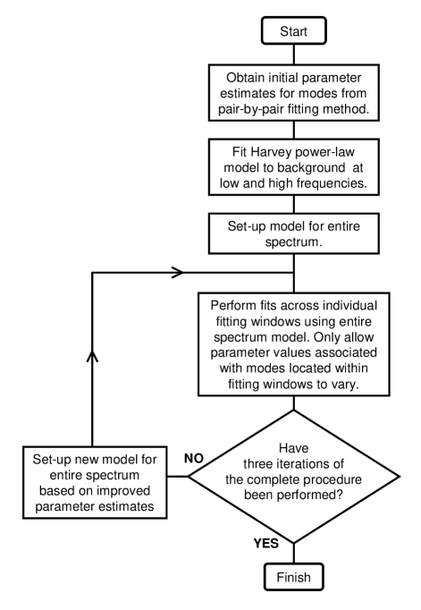
Figure 1: Step-by-step flow diagram representing the PGM fitting algorithm.

We now go on to describe the additional steps needed for the PGM, a step-by-step flow diagram of which is given in Fig. 1. The optimisation is still carried out in fitting windows with only the parameters of the modes that lie within these regions being allowed to vary. Now, however, the starting model for the fit is generated for the entire spectrum, derived from the results of an initial run of the PPM method. In this way we are accounting for any extra power arising from the wings of modes whose central frequencies lie outside the fitting window but are still optimising only a relatively small number of parameters at any one time.

There are three refinements made to the PGM used here compared to the method outlined in Paper I. The first is how we deal with asymmetries. In Paper I the simulated data contained only symmetric modes and so asymmetries were set to zero when forming the initial estimate of the full spectrum model (i.e., the impact of modes lying outside the fitting windows was based on symmetric profiles). In this work the asymmetries returned by the PPM were retained and the initial estimate of the full spectrum model was built from asymmetric modes described by Equation 2. The fact that non-zero asymmetries are used in creating the full spectrum model for the PGM is the reason why an expression such as Equation 2, which remains physically reasonable well away from the central frequencies of the modes, is needed.

The same parameters were varied in the PGM stage as were fitted in the PPM stage. However, in order to reduce the complexity of the code the sizes of the fitting windows were increased to include both an even-$\ell$ and an odd-$\ell$ mode pair (and consequently the corresponding $\ell$ = 4 and 5 modes as well). A window size of 130.1 $\mu$Hz was chosen to cover this range of modes. Since more modes were being fitted within each window, a larger number of fitting parameters was needed, however the extra computing time needed because of this is partially offset by needing fewer actual fitting windows to cover the whole spectrum.

The increased window size also meant it became more important to take account of the non-white background profile. In Paper I, a varying background that roughly mimics the granulation profile seen in real data was achieved by fitting a background parameter divided by the frequency. This time a different approach was employed. Before fitting the modes, the background was fitted at low and high frequencies, well away from the regime of the resonant modes. This fit was performed using the Harvey (1985) power-law model with an additional constant offset term to account for photon shot noise as described in $\S$ 2. From this fit the background was interpolated over the entire spectrum. Therefore, during the mode fitting stage, the background will have a non-white form as described by the fitted Harvey Model. However, in order to reduce the number of parameters only the constant offset term was allowed to vary during the mode fitting stage.

The final difference between the PGM given here and that introduced in Paper I comes in performing an extra iterative process in order to further refine the parameter estimates. By employing the PGM a more accurate set of parameters is returned compared with those estimated from the PPM. This new set of parameters was then used to set-up a more accurate full spectrum model. The entire PGM process can then be performed again to produce a further set of parameters. Tests with simulated data have shown that performing more than three iterations of this process does not bring any further significant changes in the new parameter set compared with the previous one (the difference between the fitted parameters returned from the third iteration compared with those from the second was almost always less that 0.1 sigma). Based on this we chose to perform only three iterations of the procedure in all our fits to the simulated and real data.

In terms of efficiency, the time taken to complete one complete iteration for the entire spectrum using the PGM is about three times longer than that of the PPM. Assuming three additional complete iterations are needed to produce the best fitting parameters, the overall computing time will be of the order of 10 to 15 times longer. Nevertheless, it still takes significantly less time than that which would be needed to perform a full global spectrum fit.

4 Results

The main goal of this work is to develop a better, but still computationally efficient, peak-bagging technique for real helioseismic data, and thus enable more accurate inferences about the Sun. However, in order to validate the new method, we first give the results of tests carried out on simulated data.

4.1 Simulated Data

The PPM and PGM outlined in this paper were used to fit two simulated 796-day limit spectra with GOLF-like background characteristics. It should be noted that in all the plots that follow we only give the results up to around 4000 $\mu$Hz. While we do fit at higher frequencies the parameter estimates for these modes tend to have very large uncertainties due to their short lifetimes (i.e., large linewidths). Hence, above 4000 $\mu$Hz, any improvement in the accuracy of the fits due to using the PGM is unlikely to be significant.

Fig. 2 shows the fitted estimates returned for the central frequency parameter, $\nu_{nl}$. In order to give a direct measurement of the significance of any bias in the results we have plotted the difference between the fitted values and the known input values (in the sense fitted - input) and divided by the estimated uncertainties, $\sigma_{\nu_{nl}}$. The uncertainties were calculated by taking the square root of the diagonal elements of the inverted Hessian fitting matrix. In this figure, and those that follow, different symbols have been used for different $\ell$, and open and solid symbols have been used for the PPM and PGM results respectively. Also, for the figures showing simulated data (Figs. 2 to 4) we have given plots for both the flat correlated background data (left panel) and the granulation-like correlated background data (right panel).

In both panels the plots show that there is a clear systematic bias seen in the fitted frequencies returned by the PPM. This result can be explained by the fact that asymmetric modes lying outside a particular fitting window will introduce a different level of excess power at the low frequency end of the fitting window compared with the high frequency end. Since this is not accounted for by the PPM, the fitted asymmetries will be biased and consequently affect the fitted frequencies.

The fact that fitting symmetric Lorentzian models to asymmetric modes leads to biased frequencies is well known in the literature (e.g., see Chaplin et al. 1999; Antia & Basu 1999) and so it is not surprising that inaccurate asymmetries will also lead to biased frequencies. A similar bias was seen in the frequency estimates returned in a solarFLAG “hare-and hounds” exercise when asymmetric modes were fitted, as reported in Jiménez-Reyes et al. (2008). However, in Paper I, where symmetric modes were fitted, it was shown that the PPM returned robust estimates of the frequencies. This adds further evidence that it is the inaccuracy in the asymmetries returned by the PPM that results in the biased frequencies.

Fig. 2 also shows that the bias in the frequencies returned by the PGM is significantly reduced. This is a result of the bias in the asymmetries being reduced by accounting for the offset excess power. The small amount of bias that still remains in the fitted frequencies returned by the PGM is strongly dependent on the angular degree of the modes. This is due to the fact that only a single asymmetry parameter was fitted to all the modes within a fitting window, whereas the input asymmetries actually differ slightly from mode to mode. Finally, a comparison of the two panels in Fig. 2 shows that the frequency estimates are very similar whichever background type is used.

The expected bias in the asymmetry parameter returned from the PPM is shown in Fig. 3. Again the results are plotted as the difference between the fitted and input values and divided by the uncertainties. As the asymmetries are assumed to be constant across all modes within each fitting window, we only plot one value per window. In the case of the PPM we have separate results for the $\ell$ = odd and even mode pairs, while for the PGM, where the fitting windows were increased to encompass both pairs, we only plot a single value.

A clear improvement in the fitted asymmetries returned from the PGM can be seen. For the PPM the fitted asymmetries are significantly greater than the input values by as much as 3 sigma. Since the asymmetries are negative, this actually means the PPM returns less negative values. In effect this means that the magnitudes of the fitted asymmetries are smaller than the magnitude of the input values. For the PGM any bias is consistently less than 1 sigma. Again, the results are very similar for both the flat background correlated data and the granulation-like background correlated data.

Fig. 4 shows the fitted backgrounds. Results are again shown for both the flat background correlated spectrum and the granulation-like background correlated spectrum. In these plots, in addition to showing the fits from both fitting strategies described in this paper, we also include the results of fitting the less sophisticated PGM outlined in Paper I (hereafter abbreviated OPGM).

The plots show how the background fits from the PPM overestimate the true background to a large extent. The OPGM improves upon this, but, due to not allowing for the asymmetric nature of the modes lying outside the fitting windows, a significant bias still remains. Only when using the PGM outlined in this paper are estimates much closer to the input background.

When fitting the flat background correlated spectrum, the PGM reproduces the input background very well (given by the smooth dashed lines in the plots). In the case where the input parameters are unknown, one can still make an estimate of the background in the vicinity of the modes by fitting a sensible model to low and high frequencies and interpolating (this interpolated background is given by a smooth dotted line in the plots). When a one-component Harvey model with a constant offset term to account for photon shot-noise was used to fit the flat background correlated data in this way, a very close estimate of the input was obtained.

In contrast, when the excitation functions were correlated with a granulation-like background, background fits from the PGM, while still reproducing the interpolated background well, significantly overestimated the true background. This is because the excitation function of the modes is correlated with a non-white frequency response, and as such the mode profile will increase towards low frequencies in the same manner as the background profile. This introduces an extra “pedestal” of power into the spectrum which is not accounted for by the fitting model. This pedestal also adds to the background power at low frequencies and as such will impact the interpolated background value as well.

4.2 Real Data

The PPM and PGM were also used to fit a real set of GOLF data. Although in this case we cannot test the fitted values against known input parameters, we can plot the differences between the results from the two fitting methods. This is shown for the fitted frequencies in the left panel of Fig. 5 (in the sense PGM minus PPM). We have again divided the differences by the (combined) formal uncertainties, in order to show more clearly the significance of the differences.

The plot shows that the fitted frequencies are higher when using the PGM. Also the differences appear to be largest for $\ell$ = 1 modes and smallest for $\ell$ = 3 modes. This matches what was seen when fitting the simulated limit spectrum as shown in the right panel of Fig. 5 where we have replotted the simulated results as PGM minus PPM. As with the simulated data it is likely that the different frequency estimates are a consequence of the two techniques returning different asymmetries.

Fig. 6 shows the difference in fits for the asymmetry parameter. Again we see a bias between the results returned by the PGM compared with those from the PPM. The estimates from the PGM are systematically and significantly more negative. This again matches what was seen when fitting the simulated limit spectrum as shown in the right panel of Fig. 6 where, as per the frequency plots, we have replotted the simulated data in the form PGM minus PPM.

Finally, Fig 7 shows a plot of the fitted backgrounds. We again include fits returned from the less sophisticated PGM described in Paper I. As mentioned in section 4.1 we can compare the fitted backgrounds with the background interpolated from fitting at low and high frequencies.

The fits from the PGM outlined in this paper clearly match the interpolated background better than the other two methods. However, the match is not perfect. Between about 2200 - 3100 $\mu$Hz the fitted backgrounds significantly underestimate the interpolated background wheras above 3500 $\mu$Hz there is an overestimation. The most likely source of error is in modeling the mode asymmetry, since incorrectly fitted asymmetries can have an effect on the background as seen in Fig 7.

5 Summary

We have further developed a new “pseudo-global” fitting method (PGM) designed to gain the advantages of fitting simultaneously the entire Sun-as-a-star p-mode spectrum while retaining computational efficiency. By fitting the limit spectra of simulated data it was shown that this new method enabled more accurate estimates of mode frequencies and asymmetries to be returned when compared with the estimates from a solely “local” pair-by-pair fitting method (PPM).

When fitting a real set of GOLF data it was shown that there was a systematic difference between the fitted asymmetries, and consequently the fitted frequencies, returned by the PPM and PGM. It will be the subject of further work to test whether or not such systematic biases in the frequency estimates of the low-degree modes have any significant effect on inversions to infer the solar structure. Even so, from the simulated data, we would expect that the bias in the fitted frequencies returned from the PGM to be very small. As such we think it would be of benefit to employ the PGM in future analysis of Sun-as-a-star data.

Fits to the simulated data showed that, in the case of the excitation profiles of the modes being correlated with a flat background, the new PGM returned estimates of the background very close to the input values. It is also possible to estimate the background by fitting an appropriate model at low and high frequencies and then interpolating for the frequency range where the resonant modes occur. For the flat background correlated data this “interpolated” value was also shown to match the input values reasonably well. However, in the case of the excitation profiles being correlated with a granulation-like background, both the fitted values and the interpolated values overestimated the true background.

In the real GOLF data the PGM gave estimates of the background that matched much more closely the interpolated background than those from the PPM. However, although the simulated data showed there is a difference in the returned backgrounds for the two different source types used, this only shows up in comparison with the input background. As this is unknown for the real data we cannot easily distinguish whether the modes are excited via correlations with a flat background, correlations with a granulation-like background or some mixture of the two. This also means we cannot be sure whether the asymmetric profile as used in this paper (i.e., asymmetry produced solely via correlation between the modes and the background) is physically a good match for the real modes. However, the small but significant differences between the fitted background compared with the interpolated background in the regions 2200 - 3100 $\mu$Hz and above 3500 $\mu$Hz suggest we do not yet have a perfect understanding of how the modes are generated. This could be due to a lack of understanding of how the granulation-like noise behaves in the vicinity of the modes or an incomplete understanding of how asymmetric modes are generated.

At the time of writing, the PGM had been successfully adapted in order to fit gapped data. We therefore intend to employ the technique to fit BiSON data where the time series length available is of the order of 30 years.

Figure 2: Differences between the fitted and input frequencies (in the sense fitted minus input) divided by the formal uncertainties when fitting simulated limit spectra. The results for the limit spectrum created by correlating the modes with a flat background are shown in the left panel while the results for the limit spectrum created by correlating the modes with a granulation-like background are shown in the right panel. Open symbols give the estimates returned by the PPM while solid symbols give estimates returned by the PGM. Diamonds signify $\ell$ = 0 modes, triangles $\ell$ = 1, squares $\ell$ = 2 and circles $\ell$ = 3. The solid and dotted lines give the differences averaged over four consecutive modes in frequency (i.e., one mode each of $\ell$ = 0, 1, 2 and 3).

Figure 3: Differences between the fitted and input asymmetries (in the sense fitted minus input) divided by the formal uncertainties when fitting simulated limit spectra. The results for the limit spectrum created by correlating the modes with a flat background are shown in the left panel while the results for the limit spectrum created by correlating the modes with a granulation-like background are shown in the right panel. Open symbols give the results returned by the PPM with diamonds giving the estimates from $\ell$ = even windows and triangles $\ell$ = odd windows. Solid symbols give the results from the PGM across each extended fitting window (see text).

Figure 4: Estimated backgrounds when fitting simulated limit spectra. The results for the limit spectrum created by correlating the modes with a flat background are shown in the left panel while the results for the limit spectrum created by correlating the modes with a granulation-like background are shown in the right panel. Open symbols give the results returned by the PPM, bold open symbols give the results from the PGM outlined in Paper I, and solid symbols give the results from the PGM outlined in this paper. Estimates of the background at $\ell$ = 0 frequencies are given by diamonds and at $\ell$ = 1 frequencies by triangles. The dashed lines give the real input backgrounds and the dotted lines give the interpolated backgrounds.

Figure 5: Left panel: Differences between the fitted frequencies returned by the PPM and PGM routines (in the sense PGM minus PPM) divided by the combined formal uncertainties when fitting a spectrum made from a real 796-day time series of GOLF observations. Right panel: The same as in the left panel but for the simulated granulation-like noise excited data. Diamonds signify $\ell$ = 0 modes, triangles $\ell$ = 1, squares $\ell$ = 2 and circles $\ell$ = 3. The solid line gives the differences averaged over four consecutive modes in frequency (i.e., one mode each of $\ell$ = 0, 1, 2 and 3).

Figure 6: Left panel: Differences between the fitted asymmetries returned by the PPM and PGM routines (in the sense PGM minus PPM) divided by the combined formal uncertainties when fitting a spectrum made from a real 796-day time series of GOLF observations. Right panel: The same as in the left panel but for the simulated granulation-like noise excited data. Diamonds signify the differences between asymmetry fits in the $\ell$ = even windows compared with the PGM fits and triangles signify the differences between asymmetry fits in the $\ell$ = odd windows and the PGM fits. A dotted line joins the points to aid the eye.

Figure 7: Estimated backgrounds when fitting a spectrum made from a real 796-day time series of GOLF observations. Open symbols give the results returned by the PPM, bold open symbols give the results from the PGM outlined in Paper I, and solid symbols give the results from the PGM outlined in this paper. Estimates of the background at $\ell$ = 0 frequencies are given by diamonds and at $\ell$ = 1 frequencies by triangles. The dotted line gives the interpolated background.

References

- Anderson et al. (1990) Anderson, E. R., Duvall, Jr., T. L., & Jefferies, S. M. 1990, ApJ, 364, 699
- Antia & Basu (1999) Antia, H. M., & Basu, S. 1999, ApJ, 519, 400
- Bahcall et al. (2005) Bahcall, J. N., Serenelli, A. M., & Basu, S. 2005, ApJ, 621, L85
- Chaplin et al. (2006) Chaplin, W. J., Appourchaux, T., Baudin, F., Boumier, P., Elsworth, Y., Fletcher, S. T., Fossat, E., García, R. A., Isaak, G. R., Jiménez, A., Jiménez-Reyes, S. J., Lazrek, M., Leibacher, J. W., Lochard, J., New, R., Pallé, P., Régulo, C., Salabert, D., Seghouani, N., Toutain, T., & Wachter, R. 2006, MNRAS, 369, 985
- Chaplin et al. (2008) Chaplin, W. J., Elsworth, Y., Fletcher, S. T., New, R., & Toutain, T. 2008, MNRAS, 389, 1780
- Chaplin et al. (1997) Chaplin, W. J., Elsworth, Y., Howe, R., Isaak, G. R., McLeod, C. P., Miller, B. A., & New, R. 1997, MNRAS, 287, 51
- Chaplin et al. (1999) Chaplin, W. J., Elsworth, Y., Isaak, G. R., Miller, B. A., & New, R. 1999, MNRAS, 308, 424
- Duvall et al. (1993) Duvall, Jr., T. L., Jefferies, S. M., Harvey, J. W., Osaki, Y., & Pomerantz, M. A. 1993, ApJ, 410, 829
- Fletcher (2007) Fletcher, S. T. 2007, Ph.D. Thesis
- Fletcher et al. (2008) Fletcher, S. T., Chaplin, W. J., Elsworth, Y., & New, R. 2008, AN, 329, 447
- Gabriel (1995a) Gabriel, A. H. 1995a, SolPhys, 162, 61
- Gabriel (1992) Gabriel, M. 1992, A&A, 265, 771
- Gabriel (1995b) —. 1995b, A&A, 302, 271
- García et al. (2005) García, R. A., Turck-Chièze, S., Boumier, P., Robillot, J. M., Bertello, L., Charra, J., Dzitko, H., Gabriel, A. H., Jiménez-Reyes, S. J., Pallé, P. L., Renaud, C., Roca Cortés, T., & Ulrich, R. K. 2005, A&A, 442, 385
- Harvey (1985) Harvey, J. 1985, in ESA SP-235: Future Missions in Solar, Heliospheric and Space Plasma Physics, ed. E. Rolfe & B. Battrick, 199–208
- Jiménez-Reyes et al. (2008) Jiménez-Reyes, S. J., Chaplin, W. J., García, R. A., Appourchaux, T., Baudin, F., Boumier, P., Elsworth, Y., Fletcher, S. T., Lazrek, M., Leibacher, J. W., Lochard, J., New, R., Régulo, C., Salabert, D., Toutain, T., Verner, G. A., & Wachter, R. 2008, MNRAS, 389, 1780
- Nigam & Kosovichev (1998) Nigam, R., & Kosovichev, A. G. 1998, ApJ, 505, L51
- Toutain et al. (2005) Toutain, T., Elsworth, Y., & Chaplin, W. J. 2005, A&A, 433, 713
- Toutain et al. (2006) —. 2006, MNRAS, 371, 1731