Lyman Break Galaxies at $z\approx 1.8-2.8$: GALEX/NUV Imaging of the Subaru Deep Field

Abstract

A photometric sample of $\sim$7100 $V<25.3$ Lyman break galaxies (LBGs) has been selected by combining Subaru/Suprime-Cam $BV$$R_{\rm C}$$i$′$z$′ optical data with deep GALEX/NUV imaging of the Subaru Deep Field. Follow-up spectroscopy confirmed 24 LBGs at $1.5\lesssim z\lesssim 2.7$. Among the optical spectra, 12 have Ly$\alpha$ emission with rest-frame equivalent widths of $\approx 5-60$Å. The success rate for identifying LBGs as NUV-dropouts at $1.5<z<2.7$ is 86%. The rest-frame UV (1700Å) luminosity function (LF) is constructed from the photometric sample with corrections for stellar contamination and $z<1.5$ interlopers (lower limits). The LF is $1.7\pm 0.1$ ($1.4\pm 0.1$ with a hard upper limit on stellar contamination) times higher than those of $z\sim 2$ BXs and $z\sim 3$ LBGs. Three explanations were considered, and it is argued that significantly underestimating low-$z$ contamination or effective comoving volume is unlikely: the former would be inconsistent with the spectroscopic sample at 93% confidence, and the second explanation would not resolve the discrepancy. The third scenario is that different photometric selection of the samples yields non-identical galaxy populations, such that some BX galaxies are LBGs and vice versa. This argument is supported by a higher surface density of LBGs at all magnitudes while the redshift distribution of the two populations is nearly identical. This study, when combined with other star-formation rate (SFR) density UV measurements from LBG surveys, indicates that there is a rise in the SFR density: a factor of $3-6$ ($3-10$) increase from $z\sim 5$ ($z\sim 6$) to $z\sim 2$, followed by a decrease to $z\sim 0$. This result, along with past sub-mm studies that find a peak at $z\sim 2$ in their redshift distribution, suggest that $z\sim 2$ is the epoch of peak star-formation. Additional spectroscopy is required to characterize the complete shape of the $z\sim 2$ LBG UV LF via measurements of AGN, stellar, and low-$z$ contamination and accurate distances.

1. INTRODUCTION

Over the past decade, the number of Lyman break galaxies (LBGs; for a review, see Giavalisco, 2002) identified at $z\sim 3-6$ has grown rapidly from deep, wide-field optical imaging surveys (e.g., Steidel et al., 1999; Bouwens et al., 2006; Yoshida et al., 2006). Follow-up spectroscopy on large telescopes has shown that this method (called the Lyman break technique or the “drop-out” method) is efficient at identifying high-$z$ star-forming galaxies. Furthermore, these studies have measured the cosmic star-formation history (SFH) at $z>3$, which is key for understanding galaxy evolution. It indicates that the star-formation rate (SFR) density is 10 or more times higher in the past than at $z\sim 0$.
Extending the Lyman break technique to $z<3$ requires deep, wide-field UV imaging from space, which is difficult. In addition, [O II] (the bluest optical nebular emission line) is redshifted into the near-infrared (NIR) for $z\gtrsim 1.5$ where high background and lower sensitivity limit surveys to small samples (e.g., Malkan et al., 1996; Moorwood et al., 2000; van der Werf et al., 2000; Erb et al., 2003). The combination of these observational limitations has made it difficult to probe $z\approx 1.5-2.5$.
One solution to the problem is the ‘BX’ method developed by Adelberger et al. (2004). This technique identifies blue galaxies that are detected in $U$, but show a moderately red $U-G$ color when the Lyman continuum break begins to enter into the $U$-band at $z\sim 2$.
Other methods have used NIR imaging to identify galaxies at $z=1-3$ via the Balmer/4000Å break. For example, selection of objects with $J-K>2.3$ (Vega) has yielded “distant red galaxies” at $z\sim 2-3$ (van Dokkum et al., 2004), and the ‘BzK’ method has found passive and star-forming (dusty and less dusty) galaxies at $z\approx 1.5-2.5$ (Daddi et al., 2004; Hayashi et al., 2007). The completeness of these methods is not as well understood as UV-selected techniques, since limited spectra have been obtained.
In this paper, the Lyman break technique is extended down to $z\sim 1.8$ with wide-field, deep NUV imaging of the Subaru Deep Field (SDF) with the Galaxy Evolution Explorer (GALEX; Martin et al., 2005). This survey has the advantage of sampling a large contiguous area, which allows for large scale structure studies (to be discussed in future work), an accurate measurement of a large portion of the luminosity function, and determining if the SFH peaks at $z\sim 2$.
In § 2, the photometric and spectroscopic observations are described. Section 3 presents the color selection criteria to produce a photometric sample of NUV-dropouts, which are objects undetected or very faint in the NUV, but present in the optical. The removal of foreground stars and low-$z$ galaxy contaminants, and the sample completeness are discussed in § 4. In § 5, the observed UV luminosity function (LF) is constructed from $\sim$7100 NUV-dropouts in the SDF, and the comoving star-formation rate (SFR) density at $z=1.8-2.8$ is determined. Comparisons of these results with previous surveys are described in § 6, and a discussion is provided in § 7. The appendix includes a description of objects with unusual spectral properties. A flat cosmology with [$\Omega_{\Lambda}$, $\Omega_{M}$, $h_{70}$] = [0.7, 0.3, 1.0] is adopted for consistency with recent LBG studies. All magnitudes are reported on the AB system (Oke, 1974).

2. OBSERVATIONS

This section describes the deep NUV data obtained (§ 2.1), followed by the spectroscopic observations (§ 2.2 and 2.4) from Keck, Subaru, and MMT (Multiple Mirror Telescope). An objective method for obtaining redshifts, cross-correlating spectra with templates, is presented (§ 2.3) and confirms that most NUV-dropouts are at $z\sim 2$. These spectra are later used in § 3.2 to define the final empirical selection criteria for $z\sim 2$ LBGs. A summary of the success rate for finding $z\sim 2$ galaxies as NUV-dropouts is included.

2.1. GALEX/NUV Imaging of the SDF

The SDF (Kashikawa et al., 2004), centered at $\alpha$(J2000) = 13^h24^m38$\fs$9, $\delta$(J2000) = +27°29′25$\farcs$9, is a deep wide-field (857.5 arcmin²) extragalactic survey with optical data obtained from Suprime-Cam (Miyazaki et al., 2002), the prime-focus camera mounted on the Subaru Telescope (Iye et al., 2004). It was imaged with GALEX in the NUV ($1750-2750$Å) between 2005 March 10 and 2007 May 29 (GI1-065) with a total integration time of 138176 seconds. A total of 37802 objects are detected in the full NUV image down to a depth of $\approx$27.0 mag (3$\sigma$, 7.5″ diameter aperture). The GALEX-SDF photometric catalog will be presented in future work. For now, objects undetected or faint ($NUV>25.5$) in the NUV are discussed.
The NUV image did not require mosaicking to cover the SDF, since the GALEX field-of-view (FOV) is larger and the center of the SDF is located at (+3.87′, +3.72″) from the center of the NUV image. The NUV spatial resolution (FWHM) is 5.25″, and was found to vary by no more than 6% across the region of interest (Morrissey et al., 2007).

2.2. Follow-up Spectroscopy

2.2.1 Keck/LRIS

When objects for Keck spectroscopy were selected, the NUV observations had accumulated 79598 seconds. Although the selection criteria and photometric catalog are revised later in this paper, a brief description of the original selection is provided, since it is the basis for the Keck sample. An initial NUV-dropout catalog (hereafter ver. 1) of sources with $NUV-B>1.5$ and $B-V<0.5$ was obtained. No aperture correction was applied to the 7.5″ aperture NUV flux and the 2″ aperture was used for optical photometry. These differ from the final selection discussed in § 3.2. The NUV 3$\sigma$ limiting magnitude for the ver. 1 catalog is 27.0 within a 3.39″ radius aperture. Postage stamps (see Figure 1) were examined for follow-up targets to ensure that they are indeed NUV-dropouts.

Figure 1.— Postage stamps for some NUV-dropouts targeted with LRIS. From left to right is NUV, $B$, and $V$. Each image is 24″ on a side and reveals that optical sources do not have a NUV counterpart. Photometric and spectroscopic information are provided in Table 1.

The Keck Low Resolution Imaging and Spectrograph (LRIS; Oke et al., 1995) was used to target candidate LBGs in multi-slit mode on 2007 January 23$-$25. The total integration times were either 3400, 3600, or 4833 seconds, and 36 NUV-dropouts were targeted within 3 slitmasks. A dichroic beam splitter was used with the 600 lines mm^-1 grism blazed at 4000Å and the 400 lines mm^-1 grating blazed at 8500Å, yielding blue (red) spectral coverage of $3500-5300$Å ($6600-9000$Å), although the coverages varied with location along the dispersion axis. The slits were 4″ to 8″ in length and 1″ in width, yielding spectral resolution of $\approx$0.9Å at 4300Å and $\approx$1.2Å at 8000Å.
Standard methods for reducing optical spectra were followed in PyRAF where an IRAF script, developed by K. Adelberger to reduce LRIS data, was used. When reducing the blue spectra, dome flat-fields were not used due to the known LRIS ghosting problem. Other LRIS users have avoided flat-fielding their blue spectra, since the CCD response is mostly flat (D. Stern, priv. comm).
HgNe arc-lamps were used for wavelength calibration of the blue side while OH sky-lines were used for the red side. Typical wavelength RMS was less than 0.1Å. For flux calibration, long-slit spectra of BD+26 2606 (Oke & Gunn, 1983) were obtained following the last observation for each night.
In the first mask, three of five alignment stars had coordinates that were randomly off by as much as 1″ from the true coordinates. These stars were taken from the USNO catalog, where as the better alignment stars were from the 2MASS catalog with a few tenths of an arcsecond offsets. This hindered accurate alignment, and resulted in a lower success rate of detection: the first mask had 7 of 12 NUV-dropouts that were not identified, while the other two masks had 2/10 and 3/14.

2.2.2 MMT/Hectospec

Spectra of NUV-dropouts from the final photometric catalog were obtained with the multifiber optical spectrograph Hectospec (Fabricant et al., 2005) on the 6.5m MMT on 2008 March 13 and April 10, 11, and 14. Compared to Keck/LRIS, MMT/Hectospec has a smaller collecting area and lower throughput in the blue, so fewer detections were anticipated. Therefore, observations were restricted to bright ($V_{\texttt{auto}}=22.0-23.0$) sources, which used 21 of 943 fibers from four configurations. Each source was observed in four, six, or seven 20-minute exposures using the 270 mm^-1 grating. This yielded a spectral coverage of $4000-9000$Å with 6Å resolution. The spectra were wavelength calibrated, and sky-subtracted using the standard Hectospec reduction pipeline (Fabricant et al., 2005). A more detailed discussion of these observations is deferred to a forthcoming paper (Ly et al. 2008, in prep.).

2.3. Spectroscopic Identification of Sources

The IRAF task, xcsao from the rvsao package (Kurtz & Mink, 1998, ver. 2.5.0), was used to cross-correlate with six UV spectral templates of LBGs. For cases with Ly$\alpha$ in emission, the composite of 811 LBGs from Shapley et al. (2003) and the two top quartile bins (in Ly$\alpha$ equivalent width) of Steidel et al. (2003) were used. For sources lacking Ly$\alpha$ emission (i.e., pure absorption-line systems), the spectra of MS 1512-cB58 (hereafter ‘cB58’) from Pettini et al. (2000), and the two lowest quartile bins of Steidel et al. (2003) were used.
When no blue features were present, the red end of the spectrum was examined. An object could still be at $z>1.5$, but at a low enough redshift for Ly$\alpha$ to be shortward of the spectral window. In this case, rest-frame NUV features, such as Fe II and Mg II, are available. Savaglio et al. (2004) provided a composite rest-frame NUV spectrum of 13 star-forming galaxies at $1.3<z<2$. For objects below $z\approx 1.5$, optical features are available to determine redshift. The composite SDSS spectra ($3500-7000$Å coverage) from Yip et al. (2004) and those provided with rvsao ($3000-7000$Å) are used for low-$z$ cases. Note that in computing redshifts, several different initial guesses were made to determine the global peak of the cross-correlation. In most cases, the solutions converged to the same redshift when the initial guesses are very different. The exceptions are classified as ‘ambiguous’.
Where spectra had poor S/N, although a redshift was obtained for the source, the reliability of identification (as given by xcsao’s $R$-value) was low ($R=2-3$). An objective test, which was performed to determine what $R$-values are reliable, was to remove the Ly$\alpha$ emission from those spectra and templates, and then re-run xcsao to see what $R$-values are obtained based on absorption line features in the spectra. Among 10 cases (from LRIS spectroscopy), 6 were reconfirmed at a similar redshift ($\Delta z=2.4\times 10^{-4}-1.5\times 10^{-3}$) with $R$-values of 2.30$-$7.07. This test indicates that a threshold of $R=2.5$ is reasonable for defining whether the redshift of a source (lacking emission lines) was determined. This cut is further supported by Kurtz & Mink (1998), who found that the success of determining redshifts at $R=2.5-3$ is $\sim$90%. However, to obtain more reliable redshifts, a more stricter $R=3.0$ threshold is adopted. If a $R=2.5$ threshold is adopted, then seven sources with $R=2.5-3$ (ID 86765, 92942, 96927, 153628, 169090, 190498, and 190947) are re-classified as ‘identified’. These redshifts are marginally significant: a few to several absorption features coincide with the expected UV lines for the best-fit redshifts of $\sim$2, but a few additional absorption lines are not evident in the low S/N data. Statistics presented below are provided for both adopted $R$-value cuts.
While some sources are classified ambiguous, it is likely that they could be at high-$z$. For example, 185177 (classified as ambiguous) could be a LBG, since it shows a weak emission line at $\sim$4500Å ($z\sim 2.7$ if Ly$\alpha$) and a few absorption lines. This source, statistics ($\sim$50% successful identification for $R=2.0-2.5$) from Kurtz & Mink (1998), and NUV-78625 (with $R=2.3$ but identified ‘by eye’ to be a $z\approx 1.6$ AGN) suggest that while a cut is placed at $R=2.5$ or $R=3.0$, it could be that some solutions with $R=2.0-3.0$ are correctly identified. An $R=3.0$ ($R=2.5$) typically corresponds to a peak of $\sim$0.25 ($\sim$0.2) in the cross correlation spectra, which is typically 3$\sigma$ ($2-3\sigma$) above the RMS in the cross-correlation (see Figure 2).

Figure 2.— Cross-correlation spectra for targets that yielded $R=2.5-3.2$ without an emission line. From top to bottom shows NUV-dropout ID 182284, 186254, 96927, and 92942. The top two have $R$-values of $\gtrsim 3.1$ and are identified as LBGs while the latter two have $R=2.6-3.0$ and are classified as ambiguous. The peak near the center of the plots represents the strongest peak in the cross-correlation.

2.3.1 LRIS Results

12 (14 with $R\geq 2.5$) LBGs are found at $1.7\lesssim z\lesssim 2.7$ out of 36 attempts. Among those, 10 show Ly$\alpha$ in emission, while 2 (4 with $R\geq 2.5$) are identified purely by UV absorption lines. Their spectra are shown in Figures LABEL:spec1 and LABEL:spec2, and Table 1 summarizes their photometric and spectroscopic properties. Contamination was found from 3 stars and 5 (7 with $R\geq 2.5$) low-$z$ galaxies (shown in Figure LABEL:spec3), corresponding to a 60% success rate (58% if $R>2.5$ is adopted). Four sources showed a single emission line, which is believed to be [O II] at $z\sim 1-1.5$, one source showed [O II], H$\beta$, and [O III] at $z\sim 0.7$, and two sources with absorption lines have $R\sim 2.5$ results with $z\sim 0.1$ and $\sim 0.5$ (these would be “ambiguous” with the $R\geq 3.0$ criterion). The success of identifying $z\sim 2$ LBGs improves with different color selection criteria that remove most interlopers (see § 3.2).
Of the remaining 16 spectra (12 with $R>2.5$ cut), 8 (4 with $R>2.5$ cut) were detected, but the S/N of the spectra was too low, and the other 8 were undetected. These objects were unsuccessful due to the short integration time of about one hour and their faintness (average $V$ magnitude of 24.2).
It is worthwhile to indicate that the fraction of LRIS spectra with Ly$\alpha$ emission is high (83%). In comparison, Shapley et al. (2003) reported that 68% of their $z\sim 3$ spectroscopic sample contained Ly$\alpha$ in emission. If the fraction of LBGs with Ly$\alpha$ emission does not increase from $z\sim 3$ to $z\sim 2$, it would imply that 5 $z\sim 2$ galaxies would not show Ly$\alpha$ in emission. Considering the difficulties with detecting Ly$\alpha$ in absorption with relatively short integration times, the above 83% is not surprising, and suggests that most of the $z>1.5$ ambiguous LRIS redshifts listed in Table 1 are correct.

2.3.2 Hectospec Results

Among 21 spectra, 7 objects (2 are AGNs) are identified ($R>3.0$; 9 if $R>2.5$) at $z>1.5$, 2 objects are stars, 1 (2 with $R>2.5$) is a $z<1.5$ interloper, and 11 are ambiguous (8 if $R>2.5$ is adopted). These MMT spectra are shown in Figures LABEL:spec4$-$LABEL:spec6, and their properties are listed in Table 1.
The spectrum of a $R_{\rm C}$$\sim$ 22 $z\sim 1.6$ LBG detected the Fe II and Mg II absorption lines, which indicates that MMT is sensitive enough to detect luminous LBGs. In fact, since the surface density of bright LBGs is low, slitmask instruments are not ideal for the bright end. However, the entire SDF can be observed with Hectospec, so all $\sim$150 $V_{\texttt{auto}}<23.0$ objects can be simultaneously observed.

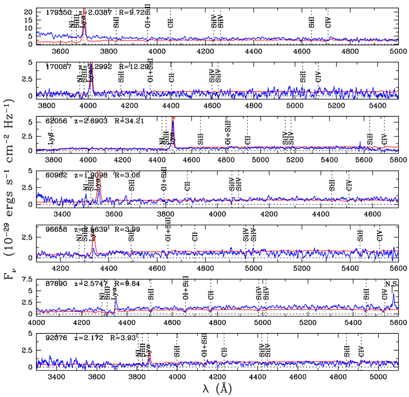
Figure 3.— LRIS spectra of confirmed NUV-dropouts from the ver. 1 catalog with known redshifts. Most of the LBGs with Ly$\alpha$ emission are shown here with the remaining in Figure LABEL:spec2. Overlayed on these spectra is the composite template (shown as grey) with the highest $R$-value (see Table 1) from cross-correlation. Note that these overlayed templates are intended to show the location of spectral features, and is not meant to compare the flux and/or the spectral index differences between the spectra and the templates. The ID number, redshifts, and $R$-values are shown in the upper left-hand corner of each panel. spec1

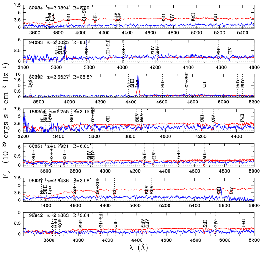
Figure 4.— Same as Figure LABEL:spec1, but some spectra do not have Ly$\alpha$ emission. The strong line seen in the spectrum of 96927 at $\sim$5570Å is a sky subtraction artifact, and cosmic rays are seen in the spectra of 94093 (at 3780Å), 186254 (at 3325Å), and 92942 (at 3990Å). These features are removed in the cross-correlation process. spec2

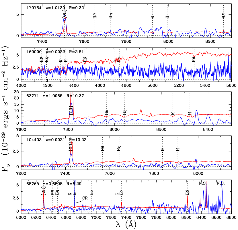
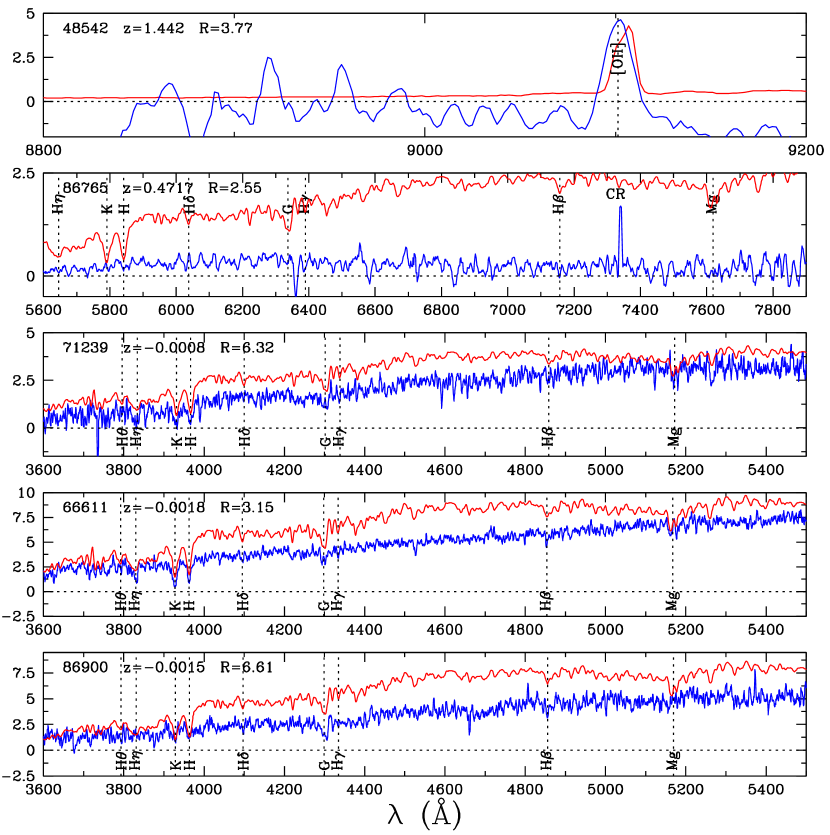
Figure 5.— Same as Figures LABEL:spec1 and LABEL:spec2, but this shows the $z<1.5$ interlopers and galactic stars. spec3

Figure 6.— Same as Figures LABEL:spec1 and LABEL:spec2, but these are Hectospec observations of LBGs in the final photometric catalog. The cross-correlation template and the typical sky spectrum are shown above and below the spectrum of the source, respectively. spec4

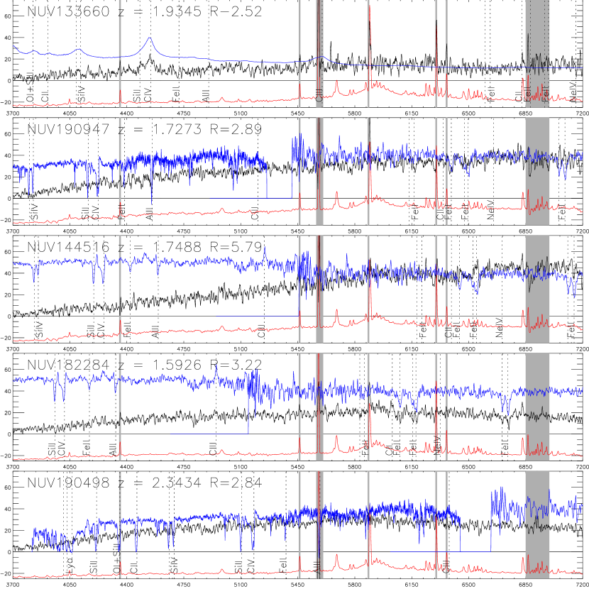
Figure 7.— Same as Figure LABEL:spec4. spec5

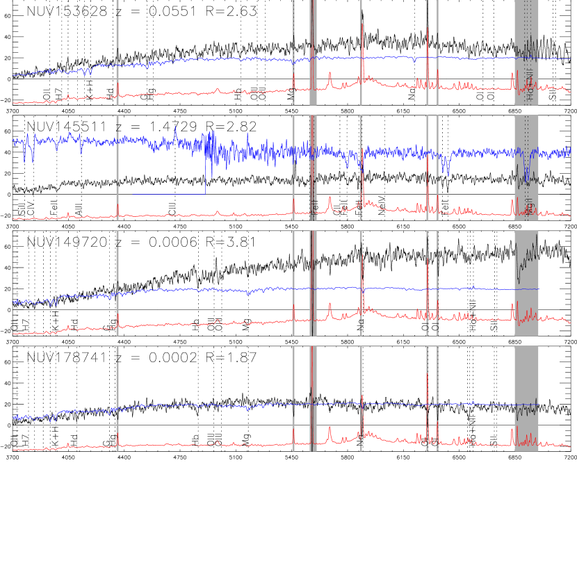
Figure 8.— Same as Figures LABEL:spec4 and LABEL:spec5, but this shows the low-$z$ interlopers and galactic stars spec6

2.4. Additional Spectra with Subaru/MOIRCS

The BzK technique, which identifies galaxies with a wide range (old and young, dusty and unreddened) of properties, could include objects that would also be classified as NUV-dropouts. As a check, cross-matching of spectroscopically identified star-forming BzK’s with the GALEX-SDF photometric catalog was performed. Spectra of BzKs were obtained on 2007 May 3$-$4 with Subaru using the Multi-Object Infrared Camera and Spectrograph (MOIRCS; Ichikawa et al., 2006). 44 sources were targeted and 15 were identified by the presence of H$\alpha$ and [N II] or [O II], [O III] and H$\beta$ emission. One of the 15 was not in the $B$-band catalog. Among the 14 objects, 7 are also classified as NUV-dropouts and were not previously identified (i.e., LRIS or Hectospec targets). This included 5 galaxies at $z>1.5$ and 2 at $z=1-1.5$. Their properties are included in Table 1. Among the 7 BzKs that did not meet the NUV-dropout criteria, 2 are below $z=1.5$ and the other five are at high-$z$. For two of the high-$z$ BzKs, one was below the $NUV-B=1.75$ cut because it is faint ($V>25.3$), thus not considered a NUV-dropout, and the other missed the $B-V=0.5$ selection by having $B-V=0.53$. The other three sources have low-$z$ neighboring sources that are detected in the NUV, which influences the NUV photometry to be brighter. The cause of confusion is due to the poor resolution of GALEX, which is discussed further in § 4.3. The details of these observations and their results are deferred to Hayashi et al. (2008).

2.5. Summary of Observations

In order to probe $1.5<z<3$ with the Lyman break technique, deep ($>$100 ks) GALEX/NUV imaging was obtained. Spectroscopic observations from Keck and MMT independently confirm that most NUV-dropouts (with their UV continuum detected spectroscopically) are found to be at $1.5<z<2.7$.
A summary of the number of LBGs, stars, and low-$z$ interlopers identified spectroscopically is provided in Table 2. Among the spectra targeting NUV-dropouts (i.e., excluding MOIRCS spectra), 53% (30/57) were identified, and among those, 63% are at $z>1.5$. Including seven objects with $R=2.5-3.0$, the percentages are 65% and 62%, respectively. These statistics are improved with the final selection criteria discussed in § 3.2.

3. Photometric Selection of NUV-dropouts

This section describes the NUV and optical photometric catalogs (§ 3.1) and the methods for merging the two catalogs. Then in § 3.2, $\sim$8000 NUV-dropouts are empirically identified with the spectroscopic sample to refine the selection criteria.

3.1. Revised NUV Photometric Catalogs

Prior to any measurements, an offset ($\Delta\alpha=-0.39$″, $\Delta\delta=-0.18$″) in the NUV image coordinates was applied to improve the astrometry for alignment with Suprime-Cam data. The scatter in the astrometric corrections was found to be $\sigma_{\Delta\alpha}$=0.39″ and $\sigma_{\Delta\delta}$=0.33″. This only results in a 0.01 mag correction for NUV measurements, and is therefore neglected.
The coordinates of $\sim$100000 SDF $B$-band sources with $B_{\texttt{auto}}<27.5$ were used to measure NUV fluxes within a 3.39″ (2.26 pixels) radius aperture with the iraf/daophot task, phot. For objects with NUV photometry below the $3\sigma$ background limit, the $3\sigma$ value is used. This limit is determined from the mode in an annulus with inner and outer radii of 22.5″ and 37.5″ (i.e., an area of 1200 pixels), respectively. For sources detected in the NUV, a point-source aperture correction of a factor of $\approx$1.83 is applied to obtain the “total” NUV flux. This correction was determined from the point spread function (PSF) of 21 isolated sources distributed across the image. The NUV catalog is then merged with the $B$-band catalog from SExtractor (SE; Bertin & Arnouts, 1996) that contains $BV$$R_{\rm C}$$i\arcmin z\arcmin$ photometry.
Throughout this paper, “total” magnitudes from the Suprime-Cam images are given by SE mag_auto, since the corrections between $B$-band Kron and the 5″ diameter magnitudes were no greater than 0.03 mag for isolated (5″ radius), point-like (SE class_star $\geq$ 0.8) targets.
The merged catalog was also corrected for galactic extinction based on the Cardelli et al. (1989) extinction law. For the SDF, they are: $A$(NUV) = 0.137, $A(B)$ = 0.067, $A(V)$ = 0.052, $A$($R_{\rm C}$) = 0.043, $A(i\arcmin)$ = 0.033, and $A(z\arcmin)$ = 0.025. Since the Galactic extinction for the SDF is low, the amount of variation in A(NUV) is no more than 0.02, so all NUV magnitudes are corrected by the same value.

3.2. Broad-band Color Selection

Using the sample of spectroscopically confirmed $z>1.5$ LBGs, low-$z$ interlopers, and stars, the color selection is optimized to minimize the number of interlopers while maximizing the number of confirmed LBGs. In Figure LABEL:select, known LBGs are identified in the $NUV-B$ versus $B-V$ diagram, where the $NUV-B$ color is given by the “total” magnitude and the $B-V$ is the color within a 2″ aperture. The latter was chosen because of the higher S/N compared to larger apertures. The final empirical selection criteria for the LBG sample are:

$$NUV-B\geq 1.75,$$ (1)

$$B-V\leq 0.50, ~{}{\rm and}$$ (2)

$$NUV-B\geq 2.4(B-V)+1.15,$$ (3)

which yielded 7964 NUV-dropouts with $21.90\leq V\leq 25.30$. Among the Hectospec and LRIS spectra, these selection criteria included all spectroscopic LBGs and excluded 4/5 stars and 4/6 (4/9 with $R>2.5$) interlopers. Therefore, the fraction of NUV-dropouts that are confirmed to be LBGs with the new selection criteria is 86% (the $R=2.5$ cut implies 79%). Note that while the $B$-band catalog was used (since the $B$ filter is closer in wavelength to the NUV), the final magnitude selection was in $V$, to compare with the rest-frame wavelength ($\approx$1700Å) of $z\sim 3$ LBGs in the $R$-band.
To summarize, a NUV-optical catalog was created, and it was combined with spectroscopic redshifts to select 7964 NUV-dropouts with $NUV-B\geq 1.75$, $B-V\leq 0.50$, $NUV-B\geq 2.4(B-V)+1.15$, and $21.90\leq V\leq 25.30$. The spectroscopic sample indicates that 14% of NUV-dropouts are definite $z\leq 1.5$ interlopers.

Figure 9.— $NUV-B$ and $B-V$ colors for $22.0<V_{\texttt{auto}}<25.3$ sources. A total of $\sim$33,000 sources are represented here, but only one-third are plotted, for clarity. Sources undetected (at the 3$\sigma$ level) in the NUV are shown as grey unfilled triangles while the detected sources are indicated as dark grey unfilled squares. Filled (unfilled) circles correspond to sources that have been confirmed as LBGs with (without) emission lines. Low-$z$ interlopers are shown as filled squares while stars are shown as unfilled stars. Skeletal stars represent Gunn-Stryker stars. select

4. CONTAMINATION AND COMPLETENESS ESTIMATES

Prior to constructing a normalized luminosity function, contaminating sources that are not LBGs must be removed statistically. Section 4.1 discusses how foreground stars are identified and removed, which was found to be a 4$-$11% correction. Section 4.2 describes the method for estimating low-$z$ contamination, and this yielded a correction of $34\%\pm 17\%$. These reductions are applied to the number of NUV-dropouts to obtain the surface density of $z\sim 2$ LBGs. Monte Carlo (MC) realizations of the data, to estimate the completeness and the effective volume of the survey, are described in § 4.3. The latter reveals that the survey samples $z\approx 1.8-2.8$.

4.1. Removal of Foreground Stars

The Gunn & Stryker (1983) stellar track passes above the NUV-dropout selection criteria box (as shown in Figure LABEL:select). This poses a problem, as objects that are undetected in the NUV can be faint foreground stars. A simple cut to eliminate bright objects is not sufficient, because faint halo stars exist in the SDF (as shown later). To reduce stellar contamination, additional photometric information from the SExtractor $BVR_{\rm c}i$′$z$′ catalogs is used. The approach of creating a “clean” sample of point-like sources, as performed by Richmond (2005), is followed. He used the class_star parameter and the difference ($\delta$) between the 2″ and 3″ aperture magnitudes for each optical image. A ‘1’ is assigned when the class_star value is $0.90-1.00$ or $0.10<\delta<0.18$, and ‘0’ otherwise for each filter. The highest score is 10 [(1+1)$\times$5], which 2623 $V_{\texttt{auto}}=21.9-26.0$ objects satisfied, and is referred to as “perfect” point-like or “rank 10” object. These rank 10 objects will be used to define the stellar locus, since contamination from galaxies is less of a problem for the most point-like sample. Then objects with lower ranks that fall close to the stellar locus will also be considered as stars after the locus has been defined.

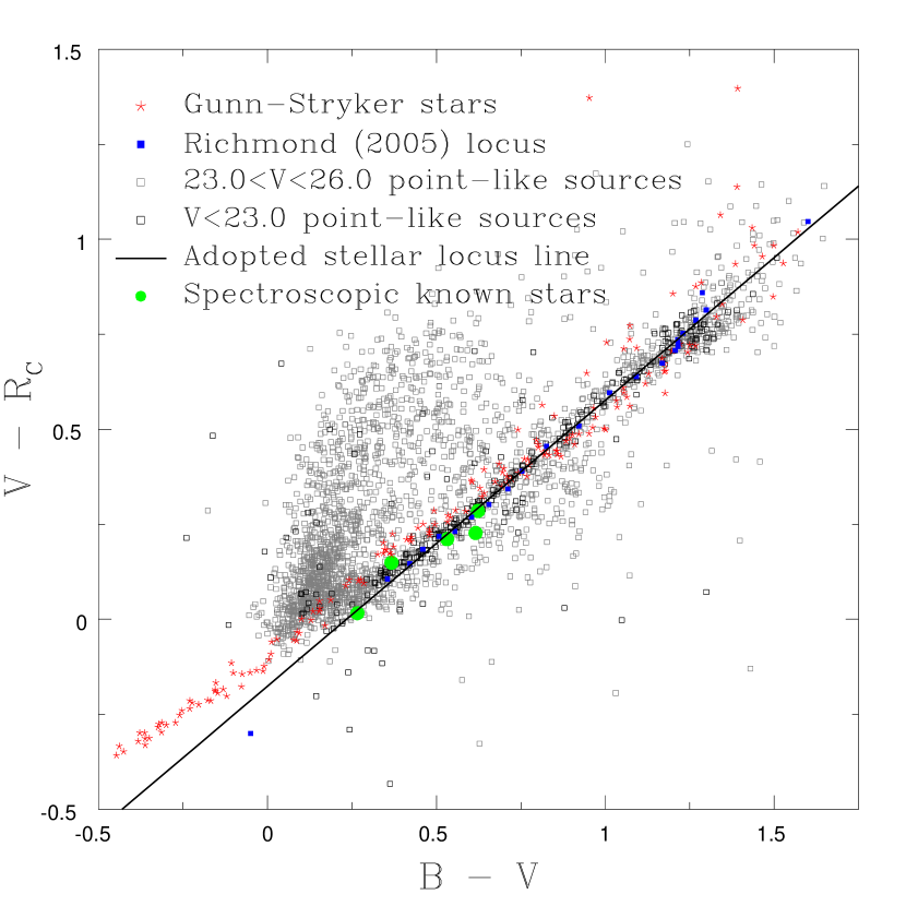
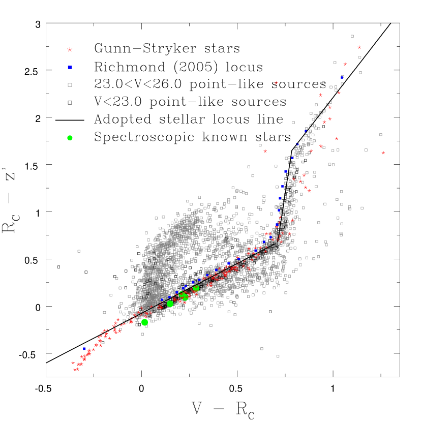
Figure 10.— Two color-color diagrams for rank 10 point-like objects. Grey (small) and black (large) squares represent sources brighter than $V_{\texttt{auto}}=26.0$ and 23.0, respectively. The Gunn-Stryker stars are shown as stars, and the SDF stellar locus of Richmond (2005) is shown as filled squares. The solid lines define the stellar locus for calculating $\Delta$ (see § 4.1). The five sources that have been spectroscopically identified to be stars are shown as filled green circles. fig3

Unfortunately, distant galaxies can also appear point-like, and must be distinguished from stars. This is done by comparing their broad-band optical colors relative to the stellar locus. Figure LABEL:fig3 shows the $B-V$, $V-R_{\rm C}$, and $R_{\rm C}-z\arcmin$ colors used in Richmond (2005) for the “clean” sample. The stellar locus is defined by the solid black lines using brighter ($V\leq 23.0$) sources. Figure LABEL:fig3 shows differences in the colors between the stellar locus defined for point-like SDF stars and those of Gunn-Stryker stars. Richmond (2005) states that this is due to metallicity, as the SDF and Gunn-Stryker stars are selected from the halo and the disk of the Galaxy, respectively.
For each object in the clean sample, the $V-R_{\rm C}$ color is used to predict the $B-V$ and $R_{\rm C}-z\arcmin$ colors along the stellar locus (denoted by ‘S.L.’ in the subscript of the colors below). These values are then compared to the observed colors to determine the magnitude deviation from the stellar locus, $\Delta=-[(B-V)_{\rm obs}-(B-V)_{\rm S.L.}]+[(R_{\rm C}-z\arcmin)_{\rm obs}-(R_{\rm C}-z\arcmin)_{\rm S.L.}]$. Therefore, an object with $\Delta\approx 0$ mag is classified as a star. This method is similar to what is done in Richmond (2005), where an object is considered a star if it is located within the stellar locus “tube” in multi-color space. This approach provides stellar contamination at faint magnitudes, which is difficult spectroscopically (Steidel et al., 2003). A histogram showing the distribution of $\Delta$ in Fig. 11a reveals two peaks: at $\Delta\approx 0$ and 0.8 mag. The comparison of $\Delta$ versus the $V$-band magnitude is shown in Fig. 11b, and a source is identified as a star if it falls within the selection criteria shown by the solid lines in this figure. A total of 1431 stars $V\leq 26.0$ are identified, while the remaining 1192 sources are classified as galaxies. The surface density as a function of magnitude for the identified stars agrees with predictions made by Robin et al. (2003) and other surface density measurements near the galactic pole. When the NUV-dropout selection criteria are applied, these numbers are reduced to 336 stars (i.e., a 4% contamination for the NUV-dropout sample) and 230 galaxies with $21.9\leq V_{\texttt{auto}}\leq 25.3$.
Sources that are ranked $7-9$ are also considered and were classified as a star or a galaxy using the above approach. Of those that met the NUV-dropout criteria, 535 and 252 have the colors of stars and galaxies, respectively. Thus, the photometric sample of NUV-dropouts contains 7093 objects after statistically removing 871 stars (11% of the NUV-dropout) that are ranked 7$-$10. The reasons for only considering objects with a rank of 7 or greater are (1) the stellar contamination does not significantly increase by including rank 6 or rank 5 objects (i.e., another 128 rank 6 stars or 1.5% and 143 rank 5 stars or 1.8%), and (2) comparison of the surface density of rank 7$-$10 stars with expectations from models showed evidence for possible contamination from galaxies at the faint end ($V>24.0$; A. Robin, priv. comm.), and the problem will worsen with rank 5 and 6 objects included. As it will be apparent later in this paper, stellar contamination is small and not expected to significantly alter any discussion of differences seen in the luminosity function. A hard upper limit by considering objects of rank 1 and above as stars would imply an additional (rank 1 to 6) stellar contamination of 14.5%.

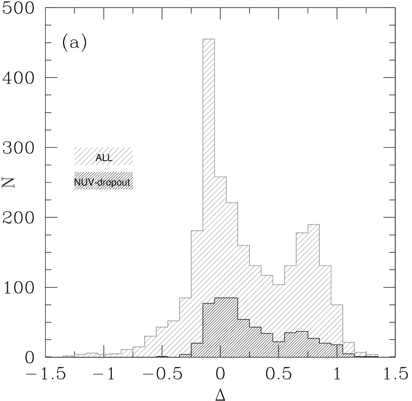
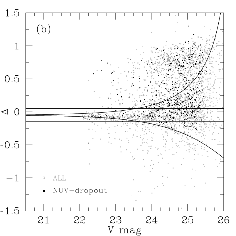
Figure 11.— Photometric properties of rank 10 point-like objects. A histogram of $\Delta$ is shown in (a) while (b) plots $\Delta$ versus $V$-band Kron magnitude. The grey histogram and squares are for all point-like sources while those that satisfy the NUV-dropout selection criteria are represented in black. The selection of foreground stars is given by the solid lines in (b). The horizontal solid lines represent a minimum $\Delta$ at the bright end while the two solid curves are the $\pm$3$\sigma$ criteria for $\Delta$, as given by $-2.5\log{[1\mp(f_{3\sigma B}^{2}+f_{3\sigma V}^{2}+f_{3\sigma R_{\rm C}}^{2}+f_{3\sigma z\arcmin}^{2})^{0.5}/f_{V}]}$. Here $f_{X}$ is the flux density in the $X$ filter.

Among the 5 sources spectroscopically determined to be stars, 3 of them (71239, 66611, and 149720) are classified as stars with the $\Delta$ method, and the other two stars (86900 and 178741) fall outside the $\Delta$ selection criteria. Among the known LBGs, 8 are rank 8$-$10 and 3 (166380, 78625, and 133660) are classified as not being stars. Since the spectroscopic sample of rank 10 objects is small, additional spectra will be required to further optimize the $\Delta$ technique. However, the spectroscopic sample (presented in this paper) indicates that $3-7\%$ of NUV-dropouts are stars, which is consistent with the $4-11\%$ derived with the $\Delta$ method.

4.2. Contamination from $z<1.5$ Interlopers

One of the biggest concerns in any survey targeting a particular redshift range is contamination from other redshifts. The spectroscopic sample of NUV-dropouts shows that 5% are definite $z<1.5$ galaxies. This number increases to an upper value of 51% if the ambiguous NUV-dropouts (that meet the color selection criteria) are all assumed to be low-$z$ interlopers. However, it is unlikely that all unidentified NUV-dropouts are low-$z$, since LBGs without Ly$\alpha$ emission in their spectra are likely missed. A secondary independent approach for estimating low-$z$ contamination, which is adopted later in this paper, is by using a sample of $z<1.5$ emission-line galaxies identified with narrow-band (NB) filters. Since a detailed description of this sample is provided in Ly et al. (2007), only a summary is given below:
A total of 5260 NB emitters are identified from their excess fluxes in the NB704, NB711, NB816, or NB921 filter either due to H$\alpha$, [O III], or [O II] emission line in 12 redshift windows (some overlapping) at $0.07\lesssim z\lesssim 1.47$. These galaxies have emission line equivalent widths and fluxes as small as 20Å (observed) and a few $\times 10^{-18}$ erg s^-1 cm^-2, and are as faint as $V=25.5-26.0$. Cross-matching was performed with the NUV-dropout sample, which yielded 487 NB emitters as NUV-dropouts. The redshift and $V$-band magnitude distributions are shown in Figure 12. Note that most of the contaminating sources are at $1.0<z<1.5$, consistent with the spectroscopic sample.

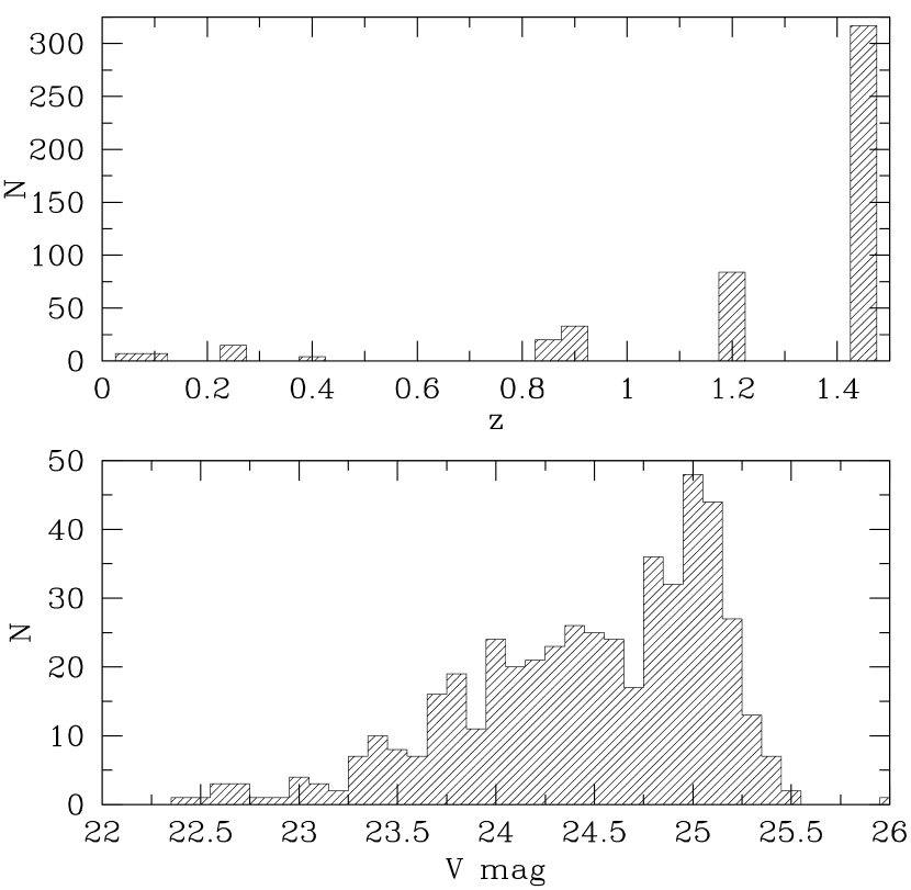
Figure 12.— Redshift (top) and $V$-band magnitude (bottom) distributions of 487 NB emitters that meet the NUV-dropout criteria. Note that the redshift bins are made larger to clearly show the histogram.

Since this sample represents a fraction of the $0.07\lesssim z\lesssim 1.5$ redshift range, the above results must be interpolated for redshifts in between the NB redshifts. It is assumed that emission-line galaxies exist at all redshifts, and possess similar properties and number densities to the NB emitters. One caveat of this approach is that blue galaxies that do not possess nebular emission lines, may meet the NUV-dropout selection. The statistics of such objects are not well known, since spectroscopic surveys are biased toward emission line galaxies, due to ease of identification. Therefore, these contamination estimates are treated as lower limits. A further discussion of this approach is provided in § 7.
Using the redshift distribution shown in Figure 12, the number of objects per comoving volume ($N/\Delta V$) is computed at each NB redshift window. For redshifts not included by the NB filters, a linear interpolation is assumed. Integrating over the volume from $z=0.08$ to $z=1.5$ yields the total number of interlopers to be $2490\pm 1260$, which corresponds to a contamination fraction of $f_{\rm contam}$= $0.34\pm 0.17$. The error on $f_{\rm contam}$ is from Poissonian statistics for each redshift bin, and are added in quadrature during the interpolation step for other redshifts. This is also determined as a function of magnitude (hereafter the “mag.-dep.” correction), since the redshift distribution will differ between the bright and faint ends. The $f_{\rm contam}$ ($V$-band magnitude range) values are $0.39\pm 0.20$ (22.9$-$23.3), $0.40\pm 0.21$ (23.3$-$23.7), $0.37\pm 0.21$ (23.7$-$24.1), $0.31\pm 0.16$ (24.1$-$24.5), $0.27\pm 0.14$ (24.5$-$24.9), and $0.39\pm 0.19$ (24.9$-$25.3).

4.3. Modelling Completeness and Effective Volume

In order to obtain an accurate LF for NUV-dropouts, the completeness of the sample must be quantified. This is accomplished with MC simulations to calculate $P(m,z)$, which is the probability that a galaxy of apparent $V$-band magnitude $m$ and at redshift $z$ will be detected in the image, and will meet the NUV-dropout color selection criteria. The effective comoving volume per solid area is then given by

$$\frac{V_{\rm eff}(m)}{\Omega}=\int dzP(m,z)\frac{dV(z)}{dz}\frac{1}{\Omega},$$ (4)

where $dV/dz/\Omega$ is the differential comoving volume per $dz$ per solid area at redshift $z$. Dividing the number of NUV-dropouts for each apparent magnitude bin by $V_{\rm eff}$ will yield the LF. This approach accounts for color selection biases, limitations (e.g., the depth and spatial resolution) of the images (Steidel et al., 1999), and choice of apertures for “total” magnitude.
In order to determine $P(m,z)$, a spectral synthesis model was first constructed from galaxev (Bruzual & Charlot, 2003) by assuming a constant SFR with a Salpeter initial mass function (IMF), solar metallicity, an age of 1Gyr, and a redshift between $z=1.0$ and $z=3.8$ with $\Delta z=0.1$ increments. The model was reddened by assuming an extinction law following Calzetti et al. (2000) with $E(B-V)=0.0-0.4$ (0.1 increments) and modified by accounting for IGM absorption following Madau (1995). The latter was chosen over other IGM models (e.g., Bershady et al., 1999) for consistency with previous LBG studies. This model is nearly identical to that of Steidel et al. (1999).
Figure 13 shows the redshift evolution of the $NUV-B$ and $B-V$ colors for this model. These models were scaled to apparent magnitudes of $V=22.0-25.5$ in increments of 0.25. These 2175 ($29\times 15\times 5$) artificial galaxies are randomly distributed across the NUV, $B$, and $V$ images with the appropriate spatial resolution (assumed to be point-like) and noise contribution with the IRAF tasks mkobject (for optical images) and addstar (using the empirical NUV PSF). Because of the poor spatial resolution of GALEX, each iteration of 435 sources (for a given $E[B-V]$ value) was divided into three sub-iterations to avoid source confusion among the mock galaxies. The artificial galaxies were then detected in the same manner as real sources. This process was repeated 100 times. Note that 21% of artificial sources did not meet the NUV-dropout criteria (see e.g., Figure LABEL:MCsim), as they were confused with one or more nearby sources detected in the NUV. This serves as an estimate for incompleteness due to confusion, and is accounted for in the final LF. These results are consistent with MOIRCS spectra that finds that $14-29$% of BzKs with $z\geq 1.5$ was missed by NUV-dropout selection criteria with nearby objects affecting the NUV flux. In addition, this simulation also revealed that among all mock LBGs with $z\leq 1.5$, 30% were photometrically scattered into the selection criteria of NUV-dropouts, which is consistent with the 34% low-$z$ contamination fraction predicted in § 4.2.
Figure LABEL:MCsim shows $P(m,z)$ as a function of magnitude for $E(B-V)=0.1$, 0.2, and $0.0-0.4$. The latter is determined from a weighted average where the $E(B-V)$ distribution from Steidel et al. (1999) is used for weighting each completeness distribution. This corresponds to an average $E(B-V)\sim 0.15$. The adopted comoving volume uses the weighted-average results. Table 3 provides the effective comoving volume per arcmin², the average redshift, the FWHM and standard deviation of the redshift distribution for subsets of apparent magnitudes.

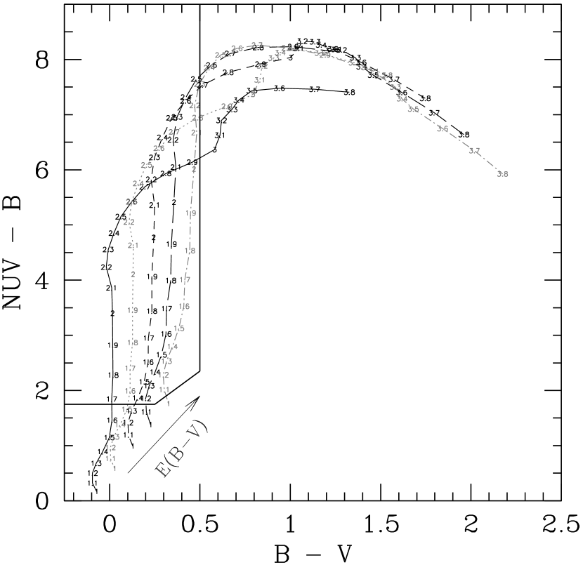
Figure 13.— Modelled $NUV-B$ and $B-V$ colors for NUV-dropouts. The solid, dotted, short-dashed, long-dashed, and dot short-dashed lines correspond to the spectral synthesis model described in § 4.3 with $E(B-V)=0.0$, 0.1, 0.2, 0.3, and 0.4, respectively. The thick solid black lines represent the selection criteria in § 3.2.

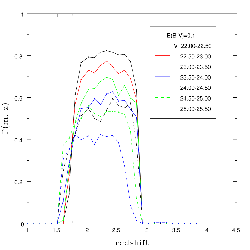
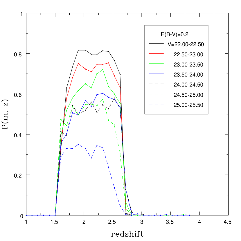
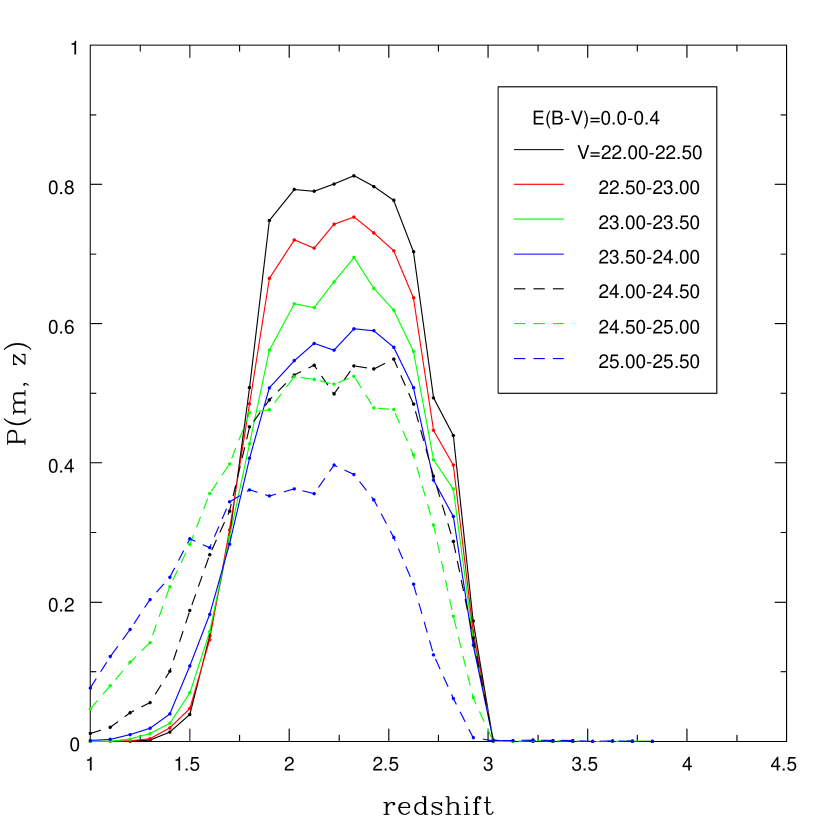
Figure 14.— Monte Carlo completeness estimates as a function of redshift for different apparent magnitude. From left to right is the result for $E(B-V)=0.1$, 0.2, and $0.0-0.4$ (a weighted average assuming the $E(B-V)$ distribution of Steidel et al., 1999). MCsim

4.4. Summary of Survey Completeness and Contamination

Using optical photometry, 871 foreground stars (i.e., a 11% correction) were identified and excluded to yield 7093 candidate LBGs. Then $z<1.5$ star-forming galaxies, identified with NB filters, were cross-matched with the NUV-dropout sample to determine the contamination fraction of galaxies at $z<1.5$. Redshifts missed by the NB filters were accounted for by interpolating the number density between NB redshifts, and this yielded $2490\pm 1260$ interlopers, or a contamination fraction of $0.34\pm 0.17$.
To determine the survey completeness, the $V_{\rm eff}$ was simulated. This consisted of generating spectral synthesis models of star-forming galaxies, and then adding artificial sources with modelled broad-band colors to the images. Objects were then detected and selected as NUV-dropouts in the same manner as the final photometric catalog. These MC simulations predict that the survey selects galaxies at $z\sim 2.28\pm 0.33$ (FWHM of $z=1.8-2.8$), and has a maximum comoving volume of $2.8\times 10^{3}~{}h_{70}^{-3}$ Mpc³ arcmin^-2.

5. RESULTS

This section provides the key measurements for this survey: a $z\sim 2$ rest-frame UV luminosity function for LBGs (§ 5.1), and by integrating this luminosity function, the luminosity and SFR densities are determined (§ 5.2).

5.1. The 1700Å UV Luminosity Function

To construct a luminosity function, a conversion from apparent to absolute magnitude is needed. The distance modulus is $m_{1700}-M_{1700}\approx 45.0$, where it is assumed that all the sources are at $z\approx 2.28$ and the K-correction term has been neglected, since it is no more than 0.08 mag. The luminosity function is given by

$$\Phi(M_{1700})=\frac{1}{\Delta m}\frac{N_{\rm raw}(1-f_{\rm contam})}{V_{\rm eff}(M_{1700})},$$ (5)

where $N_{\rm raw}$ is the raw number of NUV-dropouts within a magnitude bin ($\Delta m=0.2$), $V_{\rm eff}(M_{1700})$ is the effective comoving volume described in § 4.3, and $f_{\rm contam}$ is the fraction of NUV-dropouts that are at $z<1.5$ (see § 4.2). The photometric LF is shown in Figure LABEL:Vlf. For the mag.-dep. $f_{\rm contam}$ case, the adopted correction factor for $V\leq 22.9$ is $f_{\rm contam}$= 0.34 (the average over all magnitudes).
Converting the Schechter (1976) formula into absolute magnitude, the LF is fitted with the form:

$$\Phi(M_{1700})dM_{1700}=\frac{2}{5}\ln{(10)}\phi^{\star}x^{\alpha+1}\exp{[-x]}dM_{1700},$$ (6)

where $x\equiv 10^{-0.4(M_{1700}-M_{1700}^{\star})}$. In order to obtain the best fit, a MC simulation was performed to consider the full range of scatter in the LF. Each datapoint was perturbed randomly $5\times 10^{5}$ times following a Gaussian distribution with $1\sigma$ given by the uncertainties in $\Phi$. Each iteration is then fitted to obtain the Schechter parameters. This yielded for the mag.-dep. $f_{\rm contam}$ case: $M_{1700}^{\star}=-20.50\pm 0.79$, $\log{\phi^{\star}}=-2.25\pm 0.46$, and $\alpha=-1.05\pm 1.11$ as the best fit with 1$\sigma$ correlated errors. Since these Schechter parameters are based on lower limits of low-$z$ contamination (see § 4.2), they imply an upper limit on $\phi^{\star}$. This luminosity function is plotted onto Figure LABEL:Vlf as the solid black line, and the confidence contours are shown in Figure 16. With the faint-end slope fixed to $\alpha=-1.60$ (Steidel et al., 1999) and $-1.84$ (Reddy et al., 2008), the MC simulations yielded ($M_{1700}^{\star}$, $\log{\phi^{\star}}$) of ($-20.95\pm 0.29$, $-2.50\pm 0.17$) and ($-21.30\pm 0.35$, $-2.75\pm 0.21$), respectively.

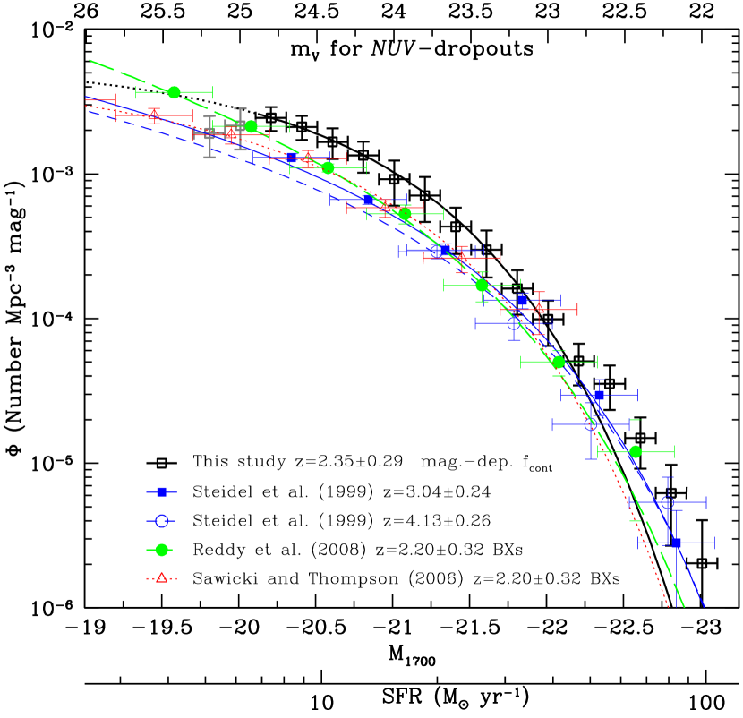
Figure 15.— The observed $V$-band luminosity function for NUV-dropouts. The LF of this work is shown by the thick black solid curve with unfilled squares. Grey points are those excluded from the MC fit. Steidel et al. (1999) measurements are shown as filled squares with solid thin curve ($z\sim 3$) and opened circles with short-dashed thin curve ($z\sim 4$). Reddy et al. (2008) BX results are shown as filled circles with long-dashed line, and Sawicki & Thompson (2006a) is represented by unfilled triangles and dotted line. Corrections to a common cosmology were made for Steidel et al. (1999) measurements, and SFR conversion follows Kennicutt (1998). Vlf

Figure 16.— Confidence contours representing the best-fitting Schechter parameters for the LF. (Top) The mag.-dep. correction where the faint-end slope is a free parameter. The vertical axes show $\alpha$ while the horizontal axes show $\log{(\phi^{\star})}$ (left) and $M^{\star}$ (right). (Bottom) $M^{\star}$ vs. $\log{(\phi^{\star})}$ for $\alpha=-1.6$ (left) and $\alpha=-1.84$ (right). The inner and outer contours represent 68% and 95% confidence levels.

5.2. The Luminosity and Star-Formation Rate Densities

The LF is integrated down to $M_{1700}=-20.11$—the magnitude where incompleteness is a problem—to obtain a comoving observed specific luminosity density (LD) of $\log{\mathcal{L}_{\rm lim}}=26.28\pm 0.69$ erg s^-1 Hz^-1 Mpc^-3 at 1700Å. The conversion between the SFR and specific luminosity for 1500-2800Å is SFR_UV(M_☉ yr^-1) = $1.4\times 10^{-28}L_{\nu}$(erg s^-1 Hz^-1), where a Salpeter IMF with masses from $0.1-100M_{\sun}$ is assumed (Kennicutt, 1998). Therefore, the extinction- (adopted $E[B-V]=0.15$ and Calzetti law) and completeness-corrected SFR density of $z\sim 2$ LBGs is $\log{\dot{\rho}_{star}}=-0.99\pm 0.69$ $M_{\sun}$ yr^-1 Mpc^-3. Using the Madau et al. (1998) conversion would decrease the SFR by $\sim$10%. Integrating to $L=0.1L^{\star}_{z=3}$, where $L^{\star}_{z=3}$ is $L^{\star}$ at $z\sim 3$ ($M^{\star}_{z=3}=-21.07$, Steidel et al., 1999), yields $\log{\mathcal{L}}=26.52\pm 0.68$ erg s^-1 Hz^-1 Mpc^-3 or an extinction-corrected SFR density of $\log{\dot{\rho}_{star}}=-0.75\pm 0.68$ $M_{\sun}$ yr^-1 Mpc^-3.

5.3. Summary of Results

A UV luminosity function was constructed and yielded a best Schechter fit of $M_{1700}^{\star}=-20.50\pm 0.79$, $\log{\phi^{\star}}=-2.25\pm 0.46$, and $\alpha=-1.05\pm 1.11$ for $z\sim 2$ LBGs. The UV specific luminosity density, above the survey limit, is $\log{\mathcal{L}_{\rm lim}}=26.28\pm 0.68$ erg s^-1 Hz^-1 Mpc^-3. Correcting for dust extinction, this corresponds to a SFR density of $\log{\dot{\rho}_{star}}=-0.99\pm 0.68$ $M_{\sun}$ yr^-1 Mpc^-3.

6. COMPARISONS WITH OTHER STUDIES

Comparisons in the UV specific luminosity densities, LFs, and Schechter parameters can be made with previous studies. First, a comparison is made between the $z\sim 2$ LBG LF with $z\sim 2$ BX and $z\sim 3$ LBG LFs. Then a discussion of the redshift evolution in the UV luminosity density and LF (parameterized in the Schechter form) is given in § 6.2.
The results are summarized in Figures LABEL:Vlf, 18, and 19 and Table 4. For completeness, three different UV specific luminosity densities are reported by integrating the LF down to: (1) $0.1L^{\star}_{z=3}$; (2) $L_{\rm lim}$, the limiting depth of the survey; and (3) $L=0$. The latter is the least confident, as it requires extrapolating the LF to the faint-end, where in most studies, it is not well determined.

6.1. UV-selected Studies at $z\sim 2-3$

In Figure LABEL:Vlf, the $z\sim 2$ LBG LF at the bright end is similar to those of LBGs from Steidel et al. (1999) and BX galaxies from Sawicki & Thompson (2006a) and Reddy et al. (2008); however, the faint end is systematically higher. This is illustrated in Figure 17 where the ratios between the binned $z\sim 2$ UV LF and the fitted Schechter forms of Steidel et al. (1999) and Reddy et al. (2008) are shown. When excluding the four brightest and two faintest bins, the NUV-dropout LF is a factor of $1.7\pm 0.1$ with respect to $z\sim 3$ LBGs of Steidel et al. (1999) and $z\sim 2$ BX galaxies of Reddy et al. (2008) and Sawicki & Thompson (2006a). The hard upper limit for stellar contamination (see § 4.1) would reduce this discrepancy to a factor of $1.4\pm 0.1$. There appears to be a trend that the ratio to Reddy et al. (2008) LF increases towards brighter magnitudes. This is caused by the differences in the shape of the two LFs, particularly the faint-end slope. The increase in the ratio is less noticeable when compared to Steidel et al. (1999), which has a shallower faint-end slope. Since the LFs of Sawicki & Thompson (2006a) and Reddy et al. (2008) are similar, the comparison of any results between the NUV-dropout and the BX selections will be made directly against Reddy et al. (2008).
All 11 points are $1-3\sigma$ from a ratio of 1. It has been assumed in this comparison that the amount of dust extinction does not evolve from $z\sim 3$ to $z\sim 2$. Evidence supporting this assumption is: in order for the intrinsic LBG LFs at $z\sim 2$ and 3 to be consistent, the population of LBGs at $z\sim 2$ would have to be relatively less reddened by $\Delta E(B-V)=0.06$ (i.e., $E[B-V]=0.09$ assuming a Calzetti extinction law). However, the stellar synthesis models, described previously, indicate that $E(B-V)$ = 0.1 star-forming galaxies are expected to have observed $B-V\sim 0.1$, and only 15% of NUV-dropouts have $B-V\leq 0.1$. This result implies that dust evolution is unlikely to be the cause for the discrepancy seen in the LFs.

Figure 17.— Comparisons of the LBG LF with other LFs. The ratios of the $z\sim 2$ LBG LF to the Schechter fits of Steidel et al. (1999) LF and Reddy et al. (2008) are shown in the top and bottom panels, respectively. On average, the $z\sim 2$ LBG LF is a factor of $1.7\pm 0.1$ higher than these studies.

To compare the luminosity densities, the binned LF is summed. This is superior to integrating the Schechter form of the LF as (1) no assumptions are made between individual LF values and for the faint-end, and (2) the results do not suffer from the problem that Schechter parameters are affected by small fluctuations at the bright- and faint-ends. The logarithm of the binned luminosity densities for $-22.91<M_{1700}<-20.11$ are $26.27\pm 0.16$ (this work), $26.02\pm 0.04$ (Steidel et al., 1999), and $26.08\pm 0.07$ ergs s^-1 Hz^-1 Mpc^-3 (Reddy et al., 2008), which implies that the $z\sim 2$ LBG UV luminosity density is $0.25\pm 0.16$ dex higher than the other two studies at the 85% confidence level.
Since the low-$z$ contamination fraction is the largest contributor to the errors, more follow-up spectroscopy will reduce uncertainties on the LF. This will either confirm or deny with greater statistical significance that the luminosity density and LF of $z\sim 2$ LBGs are higher than the $z\sim 3$ LBGs and $z\sim 2$ BXs.

6.2. Evolution in the UV Luminosity Function and Density

The Schechter LF parameters, listed in Table 4, are plotted as a function of redshift in Figure 18. There appears to be a systematic trend that $M^{\star}$ is less negative (i.e., a fainter $L^{\star}$) by $\approx$1 mag at higher redshifts for surveys with $\alpha\leq-1.35$. No systematic evolution is seen for $\phi^{\star}$, given the measurement uncertainties. Limited information are available on the faint-end slope, so no analysis on its redshift evolution is provided. It is often difficult to compare Schechter parameters, since they are correlated, and without confidence contours for the fits of each study, the apparent evolution could be insignificant. A more robust measurement is the product ($\phi^{\star}\times L^{\star}$), which is related to the luminosity density.
The observed LDs, integrated to $0.1L^{*}_{z=3}$, show a slight increase of $\approx 0.5$ dex from $z\sim 6$ to $z\sim 3$. However, the two other luminosity densities appear to be flat, given the scatter in the measurements of $\approx 0.5-1.0$ dex. A comparison between $z\sim 2$ and $z\sim 5$ studies reveal a factor of $3-6$ higher luminosity density at $z\sim 2$. The extinction-corrected results for $L_{\rm lim}=0$ and $L_{\rm lim}=0.1L^{*}_{z=3}$ show a factor of 10 increase from $z\sim 6$ Bouwens et al. (2007)’s measurement to $z\sim 2$. Bouwens et al. (2007) assumed a lower dust extinction correction. If an average $E(B-V)=0.15$ with a Calzetti law is adopted, the rise in the extinction-corrected luminosity density is $\approx 3$.

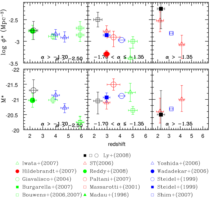
Figure 18.— Compiled Schechter parameters of LBG and BX studies versus redshift. Top and bottom show the the normalization ($\phi^{\star}$), and the “knee” of the UV LF ($M^{\star}$), respectively. Measurements are grouped according to $\alpha$: $\leq-1.70$, between $-1.70$ and $-1.35$, and $>-1.35$. This NUV-dropout work is shown as black filled square ($\alpha=-1.05$). The color and symbol conventions for studies in Figure LABEL:Vlf are identical for this figure. In the legend, Sawicki & Thompson (2006a) is abbreviated as “ST(2006)”. Some points are not shown here but have luminosity density measurements presented in Figure 19.

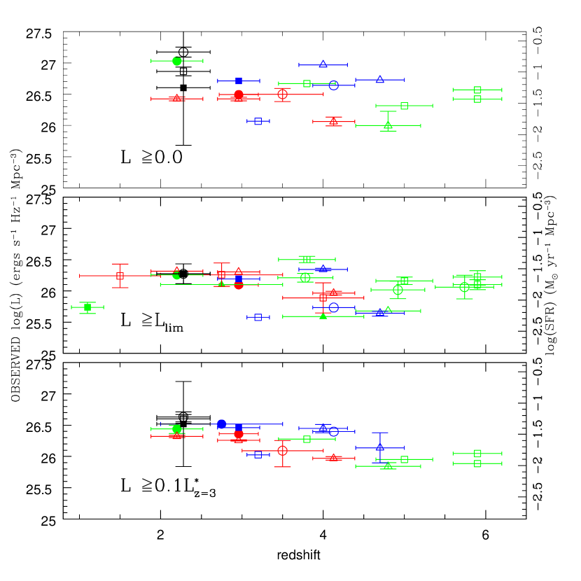
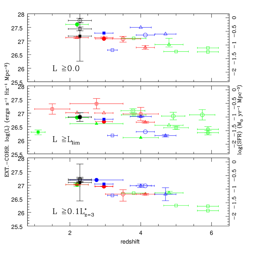
Figure 19.— The observed (left) and extinction-corrected (right) UV specific luminosity densities as a function of redshift. The luminosity function is integrated to three different limits: $L=0$ (top panel), $L=L_{\rm lim}$ (the survey’s limit; middle panel), and $L=0.1L^{*}_{z=3}$. The color and point-type schemes are the same as Figure 18. The SFR densities are shown on the right axes following Kennicutt (1998) conversion. For the $z\sim 2$ LBG luminosity density integrated to $L=L_{\rm lim}$, only one value is shown, since all the fits with different $\alpha$ are almost identical.

7. DISCUSSION

In this section, the discrepancy between the UV LF of this study and two BX studies, shown in § 6.1, is examined. Three possible explanations are considered:
1. Underestimating low-$z$ contamination. To estimate contamination, a large sample of $z\lesssim 1.5$ NB emitters was cross-matched with the NUV-dropout sample. This method indicated that $34\%\pm 17\%$ of NUV-dropouts are at $z<1.5$. However, it is possible that star-forming galaxies at $z=1-1.5$ could be missed by the NB technique, but still be identified as NUV-dropouts. This would imply that the contamination rate was underestimated. To shift the NUV-dropout LF to agree with Reddy et al. (2008) and Sawicki & Thompson (2006a) would require that the contamination fraction be more than 60%. However, the spectroscopic sample has yielded a large number of genuine LBGs and a similar low-$z$ contamination (at least 21% and at most 38%). If the large (60%) contamination rate is adopted, it would imply that only 15 of 40 spectra (LRIS and Hectospec) are at $z>1.5$, which is argued against at the 93% confidence level (98% with $R=2.5$ threshold), since 24 LBGs (1.6 times as many) have been identified. Furthermore, the LRIS and Hectospec observations independently yielded similar low contamination fractions, and the MC simulation (that involved adding artificial LBGs to the images) independently suggested 30% contamination from $z\leq 1.5$.
2. Underestimating the comoving effective volume. The second possibility is that $V_{\rm eff}$ was underestimated, as the spectral synthesis model may not completely represent the galaxies in this sample, and misses $z\sim 1-1.5$ galaxies. However, a comparison between a top-hat $P(m,z)$ from $z=1.7-2.7$ versus $z=1.4-2.7$ ($z=1.0-2.7$) would only decrease number densities by $\approx 20$% (37%). Note that the latter value is consistent with $f_{\rm contam}$.
3. Differences between LBG and BX galaxies selection. This study uses the Lyman break technique while other studies used the ‘BX’ method to identify $z\sim 2$ galaxies. Because of differences in photometric selection, it is possible that the galaxy population identified by one method does not match the other, but instead, only a fraction of BX galaxies are also LBGs and vice versa. This argument is supported by the higher surface density of LBGs compared to BXs over 2.5 mag, as shown in Figure 20a. However, their redshift distributions, as shown in Figure 20b, are very similar.
This scenario would imply that there is an increase in the LF and number density of LBGs from $z\sim 3$ to $z\sim 2$, indicating that the comoving SFR density peaks at $z\sim 2$, since there is a decline towards $z\sim 0$ from UV studies (see Hopkins, 2004, and references therein). However, it might be possible that the selection (NUV$-B-V$) of $z\sim 2$ LBGs could include more galaxies than the $U_{n}GR$ color selection used to find $z\sim 3$ LBGs. Although no reason exists to believe that $z\sim 3$ LBG selection is more incomplete than at $z\sim 2$ (nor is there any evidence for such systematic incompleteness for $z>4$ LBGs), it is difficult to rule out this possibility for certain. But if so, then the SFR density might not evolve. In addition, the conclusion that $z\sim 2$ is the peak in star-formation is based on UV selection techniques, which are less sensitive at identifying dusty ($E[B-V]>0.4$) star-forming galaxies. However, spectroscopic surveys have revealed that the sub-mm galaxy population peaks at $z\approx 2.2$ (Chapman et al., 2005), which further supports the above statement that $z\sim 2$ is the epoch of peak star-formation.

Figure 20.— Surface densities and redshift distributions for $z\sim 2$ BXs and LBGs. In (a), the surface densities of LBGs and BXs are shown as circles and triangles, respectively. Both studies have stellar and low-$z$ contamination corrections applied. This figure reveals that the LBG surface density is systematically higher than the BX’s. The redshift distributions are shown in (b). The shaded (unshaded) histogram corresponds to BXs (LBGs). For the BX, the redshift distribution is obtained from Reddy et al. (2008) spectroscopic sample, while the LBG is determined from the MC simulations described in § 4.3 for all magnitudes. The similarities in redshifts surveyed by both studies and the higher surface density of LBGs indicate that the BX technique misses a fraction of LBGs.

8. CONCLUSIONS

By combining deep GALEX/NUV and optical Suprime-Cam imaging for the Subaru Deep Field, a large sample of LBGs at $z\sim 2$ has been identified as NUV-dropouts. This extends the popular Lyman break technique into the redshift desert, which was previously difficult due to the lack of deep and wide-field UV imaging from space. The key results of this paper are:

1. Follow-up spectroscopy was obtained, and 63% of identified galaxies are at $z=1.6-2.7$. This confirms that most NUV-dropouts are LBGs. In addition, MMT/Hectospec will complement Keck/LRIS by efficiently completing a spectroscopic survey of the bright end of the LF.

2. Selecting objects with $NUV-B\geq 1.75$, $B-V\leq 0.5$, and $NUV-B\geq 2.4(B-V)+1.15$ yielded 7964 NUV-dropouts with $V=21.9-25.3$. The spectroscopic sample implied that 50$-$86% of NUV-dropouts are LBGs.

3. Using broad-band optical colors and stellar classification, 871 foreground stars have been identified and removed from the photometric sample. This corresponds to a $4-11\%$ correction to the NUV-dropout surface density, which is consistent with the $3-7\%$ from limited spectra of stars presented in this paper.

4. In addition, low-$z$ contamination was determined using a photometric sample of NB emitters at $z\lesssim 1.47$. This novel technique indicated that the contamination fraction is (at least) on average $34\%\pm 17\%$, which is consistent with the spectroscopic samples and predictions from MC simulations of the survey.

5. After removing the foreground stars and low-$z$ interlopers, MC simulations were performed to estimate the effective comoving volume of the survey. The UV luminosity function was constructed and fitted with a Schechter profile with $M_{1700}^{\star}=-20.50\pm 0.79$, $\log{\phi^{\star}}=-2.25\pm 0.46$, and $\alpha=-1.05\pm 1.11$.

6. A compilation of LF and SFR measurements for UV-selected galaxies is made, and there appears to be an increase in the luminosity density: a factor of 3$-$6 ($3-10$) increase from $z\sim 5$ ($z\sim 6$) to $z\sim 2$.

7. Comparisons between NUV-dropouts with LBGs at $z\sim 3$ (Steidel et al., 1999) and BXs at $z\sim 2$ (Sawicki & Thompson, 2006a; Reddy et al., 2008) reveal that the LF is $1.7\pm 0.1$ ($1.4\pm 0.1$ if the hard upper limit of stellar contamination is adopted) times higher than these studies. The summed luminosity density for $z\sim 2$ LBGs is 1.8 times higher at 85% confidence (i.e., $0.25\pm 0.16$ dex).

8. Three explanations were considered for the discrepancy with $z\sim 2$ BX studies. The possibility of underestimating low-$z$ contamination is unlikely, since optical spectroscopy argues against the possibility of a high (60%) contamination fraction at the 93% confidence. Second, even extending the redshift range to increase the comoving volume is not sufficient to resolve the discrepancy. The final possibility, which cannot be ruled out, is that a direct comparison between BX-selected galaxies and LBG is not valid, since the selection criteria differ. It is likely that the BX method may be missing some LBGs. This argument is supported by the similar redshift distribution of BXs and LBGs, but the consistently higher surface density of LBGs over 2.5 mag.

9. If the latter holds with future reduction of low-$z$ contamination uncertainties via spectroscopy, then the SFR density at $z\sim 2$ is higher than $z\gtrsim 3$ and $z\lesssim 1.5$ measurements obtained via UV selection. Combined with sub-mm results (Chapman et al., 2005), it indicates that $z\sim 2$ is the epoch where galaxy star-formation peaks.

Appendix A Individual Sources of Special Interest

In most cases, the confirmed LBGs showed no unique spatial or spectral properties. However, 3 cases are worth mentioning in more detail.
1. SDFJ132431.8+274214.3 (179350). Upon careful examination of the 2-D spectra, it appears that the Ly$\alpha$ emission from this source is offset by $\approx$1.1″ (9 kpc at 107° east of north) from the continuum emission, which is shown in Figure LABEL:extlyaa. The extended emission appears in the individual exposures of $15-30$ minutes. The deep ($3\sigma=28.45$) $B$-band image (Figure LABEL:extlyab) reveals that there are no sources in this direction and at this distance, assuming that the continuum emission in the spectrum corresponds to the bright source in the $B$-band image. The two sources located below the bright object in Figure LABEL:extlyab are too faint for their continuum emission to be detected with LRIS. Also, absorption features seen in the 1-D spectra (see Figure LABEL:spec1a) are at nearly the same redshift as Ly$\alpha$. This indicates that the Ly$\alpha$ emission is associated with the targeted source, rather than a secondary nearby companion.

Extended Ly$\alpha$ emission galaxies are rare (e.g., Saito et al., 2006, have the largest sample of 41 objects), and the extreme cases are extended on larger ($\sim 100$ kpc) scales, such as LAB1 and LAB2 of Steidel et al. (2000). In addition, extended Ly$\alpha$ emission has been seen in some cases that show evidence for energetic galactic winds (Mas-Hesse et al., 2003). Either this source is a fortuitous discovery from a dozen spectra, or perhaps a fraction of NUV-dropouts have extended Ly$\alpha$ emission. The physical significance of this source is not discussed here, given limited information.

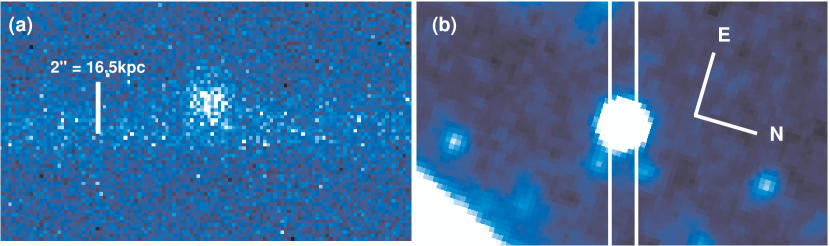
Figure 21.— Optical images for 179350. (a) The 2-D spectrum with wavelength increasing to the right shows Ly$\alpha$ emission offset by $\approx$1″ from the center of the continuum. The vertical white line corresponds to 2″. (b) The Suprime-Cam $B$-band image centered on the targeted source shows that there are no sources in the direction of the extended emission. The two white vertical lines correspond to the slit, so (b) is rotated to have the same orientation as (a), and the vertical scales are the same. extlya

2. SDFJ132452.9+272128.5 (62056). The 1- and 2-D spectra for this source reveal an asymmetric emission line, as shown in Figure LABEL:bluelyaa, but with a weak “bump” about 10Å blue-ward from the peak of Ly$\alpha$ emission. The $B$-band image (see Figure 23) shows two nearby sources where one is displaced $\approx$2″ nearly in the direction of the slit orientation while the other source is displaced in the direction perpendicular to the slit orientation. It may be possible that the blue excess is originating from the latter source due to a slight misalignment of the slit to fall between the two sources (i.e., they are physically near each other). To confirm this hypothesis, spectroscopy with a 90° rotation of the slit would show two sources with Ly$\alpha$ emission $\approx$800 km s^-1 apart.

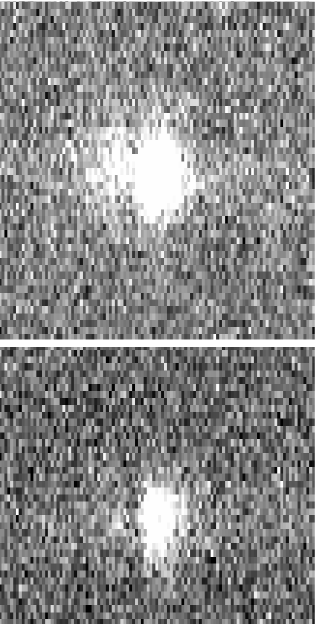
Figure 22.— (a) One- and (b) two-dimensional spectra for 62056 (top) and 72012 (bottom) centered on the Ly$\alpha$ emission. These objects appear to show weak emission blue-ward of Ly$\alpha$. See § A for a discussion. bluelya

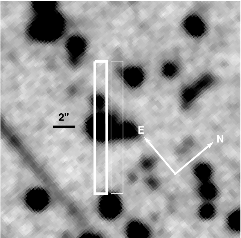
Figure 23.— The $B$-band image cropped to 20″ on a side and centered on 62056. The white box with thick lines is the LRIS slit intended to target the bright object. However, a 1.5″ offset of the slit in the north-west direction (as shown by the thin white box) may explain the blue excess seen in the 1-D and 2-D spectra (Figure LABEL:bluelya) by including both objects.

3. SDFJ132450.3+272316.24 (72012). This object is not listed in Table 1, as it was serendipitously discovered. The slit was originally targeting a narrow-band (NB) emitter. The LRIS-R spectrum showed an emission line at 7040Å, but the blue-side showed a strong emission line that appears asymmetric at $\approx$4450Å. One possibility is that the 4450Å feature is Ly$\alpha$, so that the 7040Å emission line is the redshifted C III] $\lambda$1909, but at $z=2.6634$, C III] is expected at $\approx$6994Å. This $\approx$40Å difference is not caused by poor wavelength calibration, as night sky and arc-lamps lines are located where they are expected in both the blue and red spectra. In Figure 24, the $B$-band image reveals two sources, one of which is moderately brighter in the NB704 image, as expected for a NB704 emitter. These two sources were too close for SExtractor to deblend, but the coordinate above has been corrected. Because the NB704 emitter is a foreground source, the measured NUV flux for the other source is affected, and results in a weak detected source in the NUV. Thus, this source is missed by the selection criteria of the ver. 1 catalog and those described in § 3.2. It is excluded from the spectroscopic sample discussed in § 2.

This source is of further interest because it also shows a blue excess bump (shown in Figure LABEL:bluelya) much like 62056, but weaker. This blue bump does not correspond to a different emission line with the same redshift as the 7040Å emission line. Since the bump is 10Å from the strong Ly$\alpha$ emission, it is likely associated with the source producing Ly$\alpha$. Both 62056 and 72012 were obtained on the second mask. These blue bumps are not due to a misalignment of single exposures when stacking the images together, as other equally bright sources in the mask with emission lines do not show a secondary blue peak. Other studies have also seen dual peak Ly$\alpha$ emission profiles (e.g., Tapken et al., 2004, 2007; Cooke et al., 2008; Verhamme et al., 2008). In addition, high resolution spectra of 9 LBGs have also revealed 3 cases with double-peaked Ly$\alpha$ profile (Shapley et al., 2006), which indicates that such objects may not be rare.

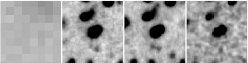
Figure 24.— Postage stamp images (10″ on a side) for 72012. From left to right is NUV, $B$, $R_{\rm C}$, and NB704. North is up and east is to the left. The source on the right shows a weak excess in NB704 relative to the broad-band images.

Table 1Properties of Spectroscopically Targeted NUV-dropouts and BzKs

$B$-band ID	Name (SDF)	UV and Optical measurements									Spectroscopic measurements
		$NUV-B$	$B-V$	$NUV$	$B$	$V$	$R_{\rm C}$	$i$′	$z$′		redshift	$R$	Temp.	F(Ly$\alpha$)	EWo(Ly$\alpha$)
(1)	(2)	(3)	(4)	(5)	(6)	(7)	(8)	(9)	(10)		(11)	(12)	(13)	(14)	(15)
With emission lines
179350L	132431.8+274214.28	$>$2.662	0.078	$>$27.121	24.459	24.366	24.379	24.430	24.500		2.0387string	9.72	45	157string	5.38string
170087L	132428.6+274037.95	$>$2.562	0.128	$>$27.126	24.564	24.498	23.991	23.880	23.859		2.2992string	12.29	45	80.4string	58.20string
string62056L	132452.9+272128.50	$>$2.991	0.107	$>$27.165	24.174	24.161	24.103	24.182	24.263		2.6903string	34.21	43,5	66.4	37.12
string60962L	132436.7+272118.67	$>$2.896	0.136	$>$27.164	24.268	24.110	23.993	23.917	23.527		1.9098string	3.06	43,5	20.3string	7.14string
string96658L	132521.5+272730.24	$>$2.605	0.282	$>$27.158	24.553	24.310	24.193	24.220	24.485		2.5639string	3.99	53,4	9.5string	5.21string
string87890L	132520.3+272559.22	$>$3.597	0.278	$>$27.161	23.564	23.334	23.298	23.335	23.362		2.5747string	9.84	23,4,5	28.9string	5.56string
string92076L	132507.6+272303.44	$>$2.666	0.239	$>$27.143	24.477	24.256	24.130	24.115	24.184		2.1720string	3.93	32,5	13.4string	6.52string
string89984L	132506.8+272620.75	$>$3.386	0.246	$>$27.169	23.783	23.567	23.516	23.436	23.309		2.0894string	3.30	21	5.6string	4.11string
string94093L	132457.7+272703.10	$>$3.248	0.129	$>$27.165	23.917	23.770	23.693	23.674	23.705		2.0025string	6.87	52,3,4	56.9string	20.71string
string82392L	132454.4+272503.97	$>$2.941	0.196	$>$27.166	24.225	24.037	24.025	24.084	24.054		2.6527string	28.57	42,3,5	112string	45.56string
139014M	132417.5+273512.63	string2.110	0.238	string26.131	24.021	23.863	23.569	23.283	23.109		1.750string	…	…	…	…
140830M	132422.4+273530.21	$>$2.816	0.100	$>$27.158	24.342	24.264	24.024	23.821	23.390		1.504string	…	…	…	…
142813M	132414.8+273552.41	$>$2.552	0.124	$>$27.160	24.608	24.420	24.401	24.194	23.647		2.018string	…	…	…	…
143960M	132425.5+273603.42	$>$2.421	0.347	$>$27.161	24.740	24.436	24.393	23.965	23.682		1.872string	…	…	…	…
166380M	132410.4+273958.51	$>$2.994	0.356	$>$27.278	24.284	23.951	23.870	23.745	23.532		2.013string	…	…	…	…
166078M	132418.2+273954.46	$>$3.332	0.530	$>$27.138	23.806	23.290	23.081	22.884	22.628		2.044string	…	…	…	…
158464M	132419.6+273842.92	string0.597	0.193	$>$25.235	24.638	24.485	24.162	23.887	23.513		1.506string	…	…	…	…
170958M	132415.8+274043.52	$>$1.136	0.495	$>$27.121	25.985	25.489	25.079	24.912	24.690		1.710string	…	…	…	…
171558M	132409.1+274052.82	string0.094	0.248	$>$25.145	25.051	24.842	24.675	24.304	23.936		1.796string	…	…	…	…
188586M	132417.8+274405.52	string1.535	0.309	string25.720	24.185	24.102	23.725	23.328	22.886		1.719string	…	…	…	…
string78625H	132343.4+272426.33	string2.625	-0.162	string25.171	22.546	22.704	22.225	22.211	22.153		1.6755string	2.30	AGN	…	…
175584H	132504.3+274147.60	string2.405	0.223	string25.284	22.879	22.643	22.341	22.084	21.723		2.3902string	2.69	43	…	…
169311H	132440.0+274040.27	$>$3.838	0.429	$>$27.142	23.304	22.949	22.847	22.890	22.875		2.6693string	6.72	31,2,4,5	…	…
144397H	132422.5+273612.47	string3.621	0.421	string26.231	22.970	22.541	22.386	22.336	22.326		2.6421string	2.60	1	…	…
133660H	132507.0+273413.84	string2.646	0.175	string25.785	23.139	22.970	23.009	22.673	22.609		1.9345string	2.52	AGN	…	…
Absorption line systems
186254L	132442.0+274334.89	$>$4.032	0.203	$>$27.145	23.113	22.910	22.833	22.727	22.560		1.7550string	3.15	62	…	…
string62351L	132447.2+272135.84	$>$3.213	0.221	$>$27.179	23.966	23.750	23.712	23.610	23.462		1.7921string	6.61	61,2	…	…
144516H	132350.8+273614.52	string1.915	0.291	string25.014	23.099	22.804	22.638	22.243	21.955		1.7488string	5.79	56	…	…
182284H	132348.4+274301.74	string3.560	0.288	string26.004	22.444	22.198	21.962	21.774	21.384		1.5926string	3.22	76	…	…
$Z<1.5$ interlopers and stars
179764L	132442.6+274220.19	string1.421	0.183	string25.673	24.252	24.054	23.970	23.602	23.391		1.0139string	9.32	[7]4,5,6	…	…
string63771L	132452.9+272147.91	$>$2.767	0.331	$>$27.163	24.396	24.058	23.832	23.383	22.922		1.0965string	10.37	[7]4,5	…	…
string68765L	132444.4+272237.13	$>$1.561	0.256	$>$27.183	25.622	25.336	24.711	24.401	24.404		0.6898string	6.29	[5]4,6,7	…	…
string48542L	132434.6+271901.63	string1.725	0.138	string26.109	24.384	24.191	23.904	23.680	23.361		1.4220string	3.77	[7]4,5	…	…
104403L	132508.4+272853.98	string1.544	0.326	string26.110	24.566	24.294	24.102	23.752	23.580		0.9921string	10.22	[7]4,5,6	…	…
136893M	132424.1+273447.28	$>$2.666	0.346	$>$27.157	24.491	24.145	23.700	23.300	22.769		1.479string	…	…	…	…
137114M	132416.4+273455.52	string1.751	0.245	string25.626	23.875	23.669	23.348	23.064	22.504		1.174string	…	…	…	…
163292M	132423.2+273923.57	string1.098	0.295	string26.278	25.180	24.875	24.544	24.263	23.777		1.498string	…	…	…	…
191435M	132422.3+274421.71	string0.673	0.119	string23.899	23.226	23.100	22.959	22.788	22.427		1.250string	…	…	…	…
145511H	132429.9+273635.92	string3.258	0.148	string25.944	22.686	22.539	22.337	22.176	21.765		1.4729string	2.82	7	…	…
string71239L	132453.1+272307.35	$>$3.984	0.623	$>$27.183	23.199	22.574	22.301	22.175	22.088		-0.0008string	6.32	[2]1,3	…	…
string66611L	132446.5+272218.81	$>$4.863	0.532	$>$27.178	22.315	21.783	21.581	21.485	21.440		-0.0018string	9.96	[2]1,3	…	…
string86900L	132511.5+272303.44	$>$4.206	0.616	$>$27.161	22.955	22.341	22.131	22.060	22.033		-0.0015string	4.65	[1]2,3	…	…
149720H	132407.7+273704.83	string3.621	0.367	string26.215	22.594	22.227	22.094	22.061	22.048		0.0006string	3.81	[9]	…	…
178741H	132515.4+274212.36	string1.760	0.266	string24.286	22.526	22.262	22.268	22.338	22.432		0.0002string	1.87	[8]	…	…
Ambiguous NUV-dropouts
185177L	132442.7+274319.52	$>$3.181	0.128	$>$27.145	23.964	23.837	23.703	23.630	23.286		2.6739	2.28	3	…	…
165834L	132431.0+273954.97	$>$4.227	0.181	$>$27.147	22.920	22.762	22.728	22.649	22.607		2.1348	2.41	1,6	…	…
string56764L	132449.4+272029.14	$>$2.591	0.159	$>$27.171	24.580	24.320	24.317	24.346	24.192		0.2473	2.49	[1]	…	…
string80830L	132503.3+272445.16	$>$2.522	0.226	$>$27.148	24.626	24.414	24.380	24.360	24.351		2.0855	2.22	[6]	…	…
string96927L	132523.0+272734.22	$>$3.255	0.190	$>$27.162	23.907	23.707	23.621	23.537	23.384		2.6436	2.98	16	…	…
											1.0713string	2.68	[3]	…	…
string92942L	132515.7+272653.97	$>$2.638	0.198	$>$27.160	24.522	24.253	24.280	24.260	24.236		2.1863	2.64	6	…	…
											0.9496string	2.44	[3]	…	…
169090L	132420.8+274025.74	$>$3.154	0.164	$>$27.137	23.983	23.798	23.660	23.461	23.223		0.0932	2.51	[2]1,3	…	…
string86765L	132453.3+272545.01	$>$2.404	0.571	$>$27.176	24.772	24.215	24.078	24.025	23.759		0.4717	2.55	[1]2,3	…	…
137763H	132406.1+273502.82	string2.547	0.102	string25.458	22.911	22.821	22.798	22.801	22.522		0.1367	1.89	[8]	…	…
string92150H	132505.3+272646.15	string3.903	0.498	string26.516	22.613	22.117	21.934	21.864	21.855		…	…	…	…	…
176626H	132352.4+274152.41	string4.172	0.482	string26.852	22.680	22.201	21.972	21.896	21.837		1.6906	2.64	6	…	…
166856H	132442.1+274005.24	$>$4.160	0.305	$>$27.286	23.126	22.820	22.625	22.469	22.137		0.0071	2.39	[1]	…	…
146434H	132524.8+273631.59	string1.864	0.091	string24.721	22.857	22.755	22.676	22.630	22.470		2.1028	2.29	6	…	…
183911H	132439.6+274311.57	string2.367	0.157	string25.361	22.994	22.821	22.562	22.396	22.043		2.0213	2.97	5	…	…
string78733H	132346.4+272426.09	string4.126	0.367	string27.164	23.038	22.683	22.586	22.567	22.575		1.8112	2.15	7	…	…
string66488H	132520.4+272220.46	$>$4.595	0.447	$>$27.165	22.570	22.126	21.960	21.897	21.833		2.4233	2.89	5	…	…
190498H	132516.9+274417.26	string3.652	0.409	string26.211	22.559	22.148	21.999	21.969	21.930		2.3434	2.84	6	…	…
											0.8932string	2.79	[3]	…	…
190947H	132346.0+274419.92	$>$4.344	0.212	$>$27.140	22.796	22.597	22.423	22.259	22.081		1.7273	2.89	3	…	…
											0.9612string	2.38	[3]	…	…
153628H	132514.5+273743.52	$>$4.563	0.457	$>$27.268	22.705	22.243	22.066	21.993	21.962		0.0551	2.63	[2]	…	…
Undetected NUV-dropouts
174747L	132436.7+274129.12	string1.951	0.247	string26.332	24.381	24.184	24.080	24.028	23.969		…	…	…	…	…
182447L	132429.1+274249.80	$>$2.603	0.385	$>$27.105	24.502	24.126	23.642	23.192	22.584		…	…	…	…	…
180088L	132421.6+274223.22	$>$2.720	0.129	$>$27.120	24.400	24.262	24.198	24.040	23.766		…	…	…	…	…
172253L	132414.3+274100.26	$>$2.911	0.224	$>$27.120	24.209	24.017	23.970	23.960	23.853		…	…	…	…	…
184387L	132414.6+274308.58	$>$2.362	0.173	$>$27.137	24.775	24.606	24.275	24.109	23.586		…	…	…	…	…
string63360L	132433.2+272142.21	$>$2.353	0.443	$>$27.167	24.814	24.275	23.840	23.600	23.346		…	…	…	…	…
113109L	132514.6+273028.10	$>$2.478	0.209	$>$27.158	24.680	24.417	24.408	24.252	24.298		…	…	…	…	…
string94367L	132459.1+272709.00	$>$3.386	0.246	$>$27.169	23.783	23.567	23.516	23.436	23.309		…	…	…	…	…

Note. — Identified sources are based on an $R>3.0$ criterion (exceptions are AGNs, stars, and those with emission lines). Col. (1) is the $B$-band catalog ID, Col. (2) is the J2000 coordinates, and magnitudes and colors are given in Cols. (3) to (10). The cross-correlated redshifts and $R$-values from xcsao are provided in Cols. (11) and (12). The template yielding the highest $R$-value is given in Col. (13), where 1-4 correspond to the four spectra of Steidel et al. (2003) from strongest Ly$\alpha$ absorption to emission, and 5 and 6 refer to the Shapley et al. (2003) composite and cB58 spectra, respectively. ‘7’ corresponds to the rest-frame NUV spectra from Savaglio et al. (2004), and ’AGN’ refers to a SDSS QSO template. For interlopers, the six SDSS composite spectra presented in Yip et al. (2004) correspond to [1] to [6] from strongest absorption-line to strongest emission-line systems. [7], [8], and [9] correspond to the rvsao templates “femtemp”, “EA”, and “eatemp”, respectively. For objects with Ly$\alpha$ emission, the line flux (in units of 10^-18 ergs s^-1 cm^-2) and rest-frame EWs (in units of Å) are given in Cols. (14) and (15), respectively. These were measured using the splot routine.

Table 2Summary of Spectroscopic Observations

Instrument	Total	LBGs [AGNs]	$z\leq 1.5$	stars	Ambiguous	Undetected
(1)	(2)	(3)	(4)	(5)	(6)	(7)
LRIS	36 (28) {4}	12 {2}	5 (1) {2}	3 (0)	8 (7) {-4}	8 (8)
Hectospec	21 (20) {3}	7 [2] {2}	1 (1) {1}	2 (1)	11 (11) {-3}	0 (0)
MOIRCS	44	10 (5)	4 (2)	0	…	…
Total	101	29 (24) [2] {4}	10 (4) {3}	5 (1)	19 (18) {-7}	8 (8)

Note. — Sources with $z>1.5$ are classified as “LBG”. Values in square brackets are those that appear to be AGNs, and those in parentheses meet the final selection criteria in § 3.2. Values in curly brackets represent LBGs that are reclassified as “identified” if a lower ($R=2.5$) threshold is adopted rather than a $R=3.0$ cut. None of the LBGs and AGNs was missed by the final selection criteria.

Table 3Effective Volume Estimates

$V$ mag	$z_{avg}$	$\sigma_{z}$	$FWHM(z)$	$V_{\rm eff}/d\Omega$	$z_{avg}$	$\sigma_{z}$	$FWHM(z)$	$V_{\rm eff}/d\Omega$	$z_{avg}$	$\sigma_{z}$	$FWHM(z)$	$V_{\rm eff}/d\Omega$
(1)	(2)	(3)	(4)	(5)	(6)	(7)	(8)	(9)	(10)	(11)	(12)	(13)
	$E(B-V)=0.0$				$E(B-V)=0.1$				$E(B-V)=0.2$
22.0-22.5	2.422	0.312	1.860$-$2.962	2.93	2.313	0.318	1.757$-$2.860	2.89	2.150	0.304	1.627$-$2.667	2.69
22.5-23.0	2.420	0.312	1.865$-$2.961	2.67	2.304	0.323	1.746$-$2.859	2.67	2.148	0.307	1.613$-$2.668	2.48
23.0-23.5	2.418	0.317	1.862$-$2.962	2.36	2.304	0.328	1.738$-$2.864	2.40	2.146	0.312	1.592$-$2.664	2.23
23.5-24.0	2.401	0.333	1.831$-$2.969	2.12	2.290	0.339	1.717$-$2.863	2.20	2.166	0.320	1.585$-$2.682	1.97
24.0-24.5	2.379	0.361	1.772$-$2.974	2.14	2.261	0.355	1.645$-$2.846	2.10	2.157	0.331	1.570$-$2.684	1.93
24.5-25.0	2.312	0.369	1.680$-$2.910	2.14	2.199	0.349	1.575$-$2.774	2.02	2.104	0.314	1.561$-$2.631	1.81
25.0-25.5	2.220	0.352	1.603$-$2.788	1.80	2.133	0.325	1.569$-$2.659	1.44	2.043	0.292	1.560$-$2.487	1.01
	$E(B-V)=0.3$				$E(B-V)=0.4$				$E(B-V)=0.0-0.4$
22.0-22.5	2.074	0.290	1.563$-$2.569	2.41	1.956	0.236	1.553$-$2.359	1.78	2.278	0.333	1.752$-$2.837	2.79
22.5-23.0	2.079	0.287	1.573$-$2.567	2.16	1.952	0.233	1.559$-$2.352	1.57	2.274	0.335	1.740$-$2.834	2.56
23.0-23.5	2.088	0.291	1.573$-$2.574	1.88	1.957	0.230	1.562$-$2.350	1.40	2.273	0.338	1.741$-$2.832	2.28
23.5-24.0	2.077	0.295	1.567$-$2.572	1.79	1.952	0.232	1.557$-$2.349	1.34	2.268	0.345	1.711$-$2.839	2.07
24.0-24.5	2.060	0.293	1.559$-$2.559	1.77	1.934	0.235	1.553$-$2.313	1.28	2.248	0.360	1.610$-$2.834	2.02
24.5-25.0	2.002	0.279	1.557$-$2.422	1.29	1.887	0.237	2.131$-$2.243	0.56	2.194	0.354	1.574$-$2.762	1.91
25.0-25.5	1.898	0.266	1.550$-$2.004	0.35	1.967	0.334	1.962$-$2.062	0.08	2.139	0.336	1.571$-$2.652	1.30

Note. — Results for MC simulations described in § 4.3 for different assumed $E(B-V)$ values. Col. (1) lists the apparent $V$-band magnitude. Cols. (2), (6), and (10) show the average redshift ($z_{avg}$), and Cols. (3), (7), and (11) list the redshift $1\sigma$ uncertainties. Cols. (4), (8), and (12) give the FWHM of the redshift distribution, and the effective comoving volume per area in units of $10^{3}$ $h_{70}^{-3}$ Mpc³ arcmin^-2 are in Cols. (5), (9), and (13).

Table 4Compilation of UV Luminosity Functions and Luminosity Densities

Reference	$z$	$N$	Area	$\lambda_{\rm rest}$	$C_{E}$	$C_{L}$	$C_{\Phi}$	$\log{\phi_{\star}}$	$M_{\star}$	$\alpha$	$\log{\mathcal{L_{\rm obs}}}$
											$L\geq 0.1L_{z=3}$	$L\geq L_{\rm lim}$	$L\geq 0$
(1)	(2)	(3)	(4)	(5)	(6)	(7)	(8)	(9)	(10)	(11)	(12)	(13)	(14)
Bouwens et al. (2006)	5.90$\pm$0.30	506	344.2	1350	1.51	1.000	1.000	-2.69${}^{+0.15}_{-0.21}$	-20.25$\pm$0.20	-1.73${}^{+0.21}_{-0.20}$	26.047	26.224${}^{+0.10}_{-0.13}$	26.567
Bouwens et al. (2007)	3.80$\pm$0.35	4671	347	1600	2.692	1.000	1.000	-2.89${}^{+0.06}_{-0.07}$	-20.98$\pm$0.10	-1.73$\pm$0.05	26.276	26.503$\pm$0.05	26.668
	5.00$\pm$0.35	1416	367	1600	1.995	1.000	1.000	-3.00${}^{+0.11}_{-0.16}$	-20.64$\pm$0.13	-1.66$\pm$0.09	25.952	26.161$\pm$0.06	26.313
	5.90$\pm$0.30	627	396	1350	1.51	1.000	1.000	-2.85${}^{+0.16}_{-0.15}$	-20.24$\pm$0.19	-1.74$\pm$0.16	25.885	26.100$\pm$0.08	26.421
Burgarella et al. (2007)	1.10$\pm$0.20	420	947	1800	3.651	1.000	1.000	…	…	…	…	25.738${}^{+0.08}_{-0.10}$	…
Foucaud et al. (2003)	3.20${}^{+0.02}_{-0.30}$	1294	1700	1900	…	1.000	1.000	…	…	…	…	…	…
Giavalisco et al. (2004)	3.78$\pm$0.34	1115	316	1500	7.48	1.000	1.000	…	…	-1.60	…	26.212$\pm$0.07	…
	4.92$\pm$0.33	275	316	1500	7.48	1.000	1.000	…	…	-1.60	…	26.017$\pm$0.14	…
	5.74$\pm$0.36	122	316	1500	7.48	1.000	1.000	…	…	-1.60	…	26.061$\pm$0.19	…
Hildebrandt et al. (2007)	2.96$\pm$0.24	14283	9.99	1650	3.88	1.000	1.000	-3.29$\pm$0.08	-22.43$\pm$0.11	-1.60	26.362	26.097	26.492
Iwata et al. (2007)	4.80$\pm$0.40	853	1290	1500	7.48	1.000	1.000	-3.39${}^{+0.23}_{-0.53}$	-21.23$\pm$0.30	-1.45${}^{+0.38}_{-0.32}$	25.841${}^{+0.06}_{-0.04}$	25.679	25.995${}^{+0.23}_{-0.09}$
Madau et al. (1996)	2.75$\pm$0.75	69	4.65	1620	3.23	1.108	0.712	…	…	…	…	$<$26.101	…
	4.00$\pm$0.50	14	4.65	1630	3.23	1.170	0.662	…	…	…	…	$<$25.588	…
Massarotti et al. (2001)	1.50$\pm$0.50	315	5.31	1500	8.10	0.980	0.844	…	…	…	…	26.240$\pm$0.19	…
	2.75$\pm$0.75	232	5.31	1500	12.17	1.108	0.712	…	…	…	…	26.259$\pm$0.19	…
	4.00$\pm$0.50	54	5.31	1500	12.00	1.170	0.662	…	…	…	…	25.889$\pm$0.24	…
Paltani et al. (2007)	3.50$\pm$0.50	113	1720	1700	3.80	1.000	1.000	-2.91${}^{+0.14}_{-0.22}$	-21.49$\pm$0.19	-1.40	26.093${}^{+0.16}_{-0.26}$	…	26.499${}^{+0.09}_{-0.12}$
Reddy et al. (2008)	2.20$\pm$0.32	10007	1925.8	1700	3.796	1.000	1.000	-2.76${}^{+0.13}_{-0.20}$	-20.97$\pm$0.23	-1.84$\pm$0.11	26.439${}^{+0.06}_{-0.07}$	26.256	27.030
Sawicki & Thompson (2006a, b)	2.20$\pm$0.32	2417	169	1700	5-15	1.000	1.000	-2.52${}^{+0.20}_{-0.26}$	-20.60${}^{+0.38}_{-0.44}$	-1.20${}^{+0.24}_{-0.22}$	26.320$\pm$0.02	26.314	26.424$\pm$0.03
	2.96$\pm$0.26	1481	169	1700	5-15	1.000	1.000	-2.77${}^{+0.13}_{-0.09}$	-20.90${}^{+0.22}_{-0.14}$	-1.43${}^{+0.17}_{-0.09}$	26.257$\pm$0.01	26.303	26.422$\pm$0.03
	4.13$\pm$0.26	427	169	1700	5-15	1.000	1.000	-3.07${}^{+0.21}_{-0.33}$	-21.00${}^{+0.40}_{-0.46}$	-1.26${}^{+0.40}_{-0.36}$	25.969$\pm$0.03	25.965$\pm$0.03	26.061$\pm$0.07
Shimasaku et al. (2005)	5.90$\pm$0.30	12	767	1425	4.358	1.000	1.000	…	…	…	…	24.447${}^{+0.11}_{-0.15}$	…
Shim et al. (2007)	3.20$\pm$0.14	1088	9468	1550	3.964	1.000	1.000	-2.81	-20.69	-0.83	26.027	25.578	26.067
Steidel et al. (1999)	2.96$\pm$0.26	1270	1046	1700	3.796	1.126	0.693	-2.86	-21.07$\pm$0.15	-1.60$\pm$0.13	26.462	26.193	26.711
	4.13$\pm$0.26	207	828	1700	3.796	1.175	0.658	-2.97	-21.11	-1.60	26.397	25.734	26.640
Wadadekar et al. (2006)	2.75$\pm$0.75	125	5.67	1850	4.70	0.862	1.249	…	…	…	26.518	…	…
Yoshida et al. (2006)	4.00$\pm$0.30	3808	875	1500	3.381	1.000	1.000	-2.84${}^{+0.11}_{-0.12}$	-21.14${}^{+0.14}_{-0.15}$	-1.82$\pm$0.09	26.450${}^{+0.06}_{-0.07}$	26.343$\pm$0.02	26.968
	4.70$\pm$0.30	539	875	1500	3.381	1.000	1.000	-2.91${}^{+0.13}_{-0.11}$	-20.72${}^{+0.16}_{-0.14}$	-1.82	26.138$\pm$0.24	25.645${}^{+0.03}_{-0.05}$	26.726
This work	2.28$\pm$0.33	7093	857.5	1700	3.796	1.000	1.000	-2.25$\pm$0.46	-20.50$\pm$0.79	-1.05$\pm$1.11	26.519$\pm$0.68	26.276$\pm$0.68	26.601$\pm$0.92
								-2.50$\pm$0.17	-20.95${}^{+0.43}_{-0.29}$	-1.60	26.601$\pm$0.07	26.293$\pm$0.07	26.864$\pm$0.07
								-2.75$\pm$0.21	-21.30$\pm$0.35	-1.84	26.633$\pm$0.08	26.305$\pm$0.08	27.172$\pm$0.08

Note. — Cols. (1) through (5) list the reference, the redshift, the sample size, the area (arcmin²), and the rest-wavelength of measurements (Å). Dust extinction correction is provided in Col. (6), and corrections to a common cosmology for luminosity and number density are shown in Cols. (7) and (8) . Schechter LF parameters are listed in Cols. (9)-(11) in units of Mpc^-3 for number density, and finally the observed luminosity densities (erg s^-1 Hz^-1 Mpc^-3) are provided in Cols. (12)-(14) for three different limits of integration.

References

- Adelberger et al. (2004) Adelberger, K. L., Steidel, C. C., Shapley, A. E., Hunt, M. P., Erb, D. K., Reddy, N. A., & Pettini, M. 2004, ApJ, 607, 226
- Bershady et al. (1999) Bershady, M. A., Charlton, J. C., & Geoffroy, J. M. 1999, ApJ, 518, 103
- Bertin & Arnouts (1996) Bertin, E., & Arnouts, S. 1996, A&AS, 117, 393
- Bouwens et al. (2006) Bouwens, R. J., Illingworth, G. D., Blakeslee, J. P., & Franx, M. 2006, ApJ, 653, 53
- Bouwens et al. (2007) Bouwens, R. J., Illingworth, G. D., Franx, M., & Ford, H. 2007, ApJ, 670, 928
- Burgarella et al. (2007) Burgarella, D., et al. 2007, MNRAS, 380, 986
- Bruzual & Charlot (2003) Bruzual, G., & Charlot, S. 2003, MNRAS, 344, 1000
- Calzetti et al. (2000) Calzetti, D., Armus, L., Bohlin, R. C., Kinney, A. L., Koornneef, J., & Storchi-Bergmann, T. 2000, ApJ, 533, 682
- Cardelli et al. (1989) Cardelli, J. A., Clayton, G. C., & Mathis, J. S. 1989, ApJ, 345, 245
- Chapman et al. (2005) Chapman, S. C., Blain, A. W., Smail, I., & Ivison, R. J. 2005, ApJ, 622, 772
- Cooke et al. (2008) Cooke, J., Barton, E. J., Bullock, J. S., Stewart, K. R., & Wolfe, A. M. 2008, ApJ, 681, L57
- Daddi et al. (2004) Daddi, E., Cimatti, A., Renzini, A., Fontana, A., Mignoli, M., Pozzetti, L., Tozzi, P., & Zamorani, G. 2004, ApJ, 617, 746
- Erb et al. (2003) Erb, D. K., Shapley, A. E., Steidel, C. C., Pettini, M., Adelberger, K. L., Hunt, M. P., Moorwood, A. F. M., & Cuby, J.-G. 2003, ApJ, 591, 101
- Fabricant et al. (2005) Fabricant, D., et al. 2005, PASP, 117, 1411
- Foucaud et al. (2003) Foucaud, S., et al. 2003, A&A, 409, 835
- Giavalisco (2002) Giavalisco, M. 2002, ARA&A, 40, 579
- Giavalisco et al. (2004) Giavalisco, M., et al. 2004, ApJ, 600, L103
- Gunn & Stryker (1983) Gunn, J. E., & Stryker, L. L. 1983, ApJS, 52, 121
- Hayashi et al. (2007) Hayashi, M., Shimasaku, K., Motohara, K., Yoshida, M., Okamura, S., & Kashikawa, N. 2007, ApJ, 660, 72
- Hayashi et al. (2008) Hayashi, M., et al. 2009, ApJ, 691, 140
- Hopkins (2004) Hopkins, A. M. 2004, ApJ, 615, 209
- Mas-Hesse et al. (2003) Mas-Hesse, J. M., Kunth, D., Tenorio-Tagle, G., Leitherer, C., Terlevich, R. J., & Terlevich, E. 2003, ApJ, 598, 858
- Hildebrandt et al. (2007) Hildebrandt, H., et al. 2007, A&A, 462, 865
- Ichikawa et al. (2006) Ichikawa, T., et al. 2006, Proc. SPIE, 6269,
- Iwata et al. (2007) Iwata, I., Ohta, K., Tamura, N., Akiyama, M., Aoki, K., Ando, M., Kiuchi, G., & Sawicki, M. 2007, MNRAS, 376, 1557
- Iye et al. (2004) Iye, M., et al. 2004, PASJ, 56, 381
- Kashikawa et al. (2004) Kashikawa, N., et al. 2004, PASJ, 56, 1011
- Kennicutt (1998) Kennicutt, R. C. 1998, ARA&A, 36, 189
- Kurtz & Mink (1998) Kurtz, M. J., & Mink, D. J. 1998, PASP, 110, 934
- Ly et al. (2007) Ly, C., et al. 2007, ApJ, 657, 738
- Madau (1995) Madau, P. 1995, ApJ, 441, 18
- Madau et al. (1996) Madau, P., Ferguson, H. C., Dickinson, M. E., Giavalisco, M., Steidel, C. C., & Fruchter, A. 1996, MNRAS, 283, 1388
- Madau et al. (1998) Madau, P., Pozzetti, L., & Dickinson, M. 1998, ApJ, 498, 106
- Malkan et al. (1996) Malkan, M. A., Teplitz, H., & McLean, I. S. 1996, ApJ, 468, L9
- Martin et al. (2005) Martin, D. C., et al. 2005, ApJ, 619, L1
- Massarotti et al. (2001) Massarotti, M., Iovino, A., & Buzzoni, A. 2001, ApJ, 559, L105
- Miyazaki et al. (2002) Miyazaki, S., et al. 2002, PASJ, 54, 833
- Moorwood et al. (2000) Moorwood, A. F. M., van der Werf, P. P., Cuby, J. G., & Oliva, E. 2000, A&A, 362, 9
- Morrissey et al. (2007) Morrissey, P., et al. 2007, ApJS, 173, 682
- Oke (1974) Oke, J. B. 1974, ApJS, 27, 21
- Oke & Gunn (1983) Oke, J. B., & Gunn, J. E. 1983, ApJ, 266, 713
- Oke et al. (1995) Oke, J. B., et al. 1995, PASP, 107, 375
- Paltani et al. (2007) Paltani, S., et al. 2007, A&A, 463, 873
- Pettini et al. (2000) Pettini, M., Steidel, C. C., Adelberger, K. L., Dickinson, M., & Giavalisco, M. 2000, ApJ, 528, 96
- Reddy et al. (2008) Reddy, N. A., Steidel, C. C., Pettini, M., Adelberger, K. L., Shapley, A. E., Erb, D. K., & Dickinson, M. 2008, ApJS, 175, 48
- Richmond (2005) Richmond, M. 2005, PASJ, 57, 969
- Robin et al. (2003) Robin, A. C., Reylé, C., Derrière, S., & Picaud, S. 2003, A&A, 409, 523
- Saito et al. (2006) Saito, T., Shimasaku, K., Okamura, S., Ouchi, M., Akiyama, M., & Yoshida, M. 2006, ApJ, 648, 54
- Savaglio et al. (2004) Savaglio, S., et al. 2004, ApJ, 602, 51