Euclidean Epstein-Glaser Renormalization

Abstract

In the framework of perturbative Algebraic Quantum Field Theory (pAQFT) recently developed by Brunetti, Dütsch, and Fredenhagen (arXiv:0901.2038), I give a general construction of so-called “Euclidean time-ordered products”, i.e. algebraic versions of the Schwinger functions, for scalar quantum field theories on spaces of Euclidean signature. This is done by generalizing the recursive construction of time-ordered products by Epstein and Glaser, originally formulated for quantum field theories on Minkowski space (MQFT). An essential input of Epstein-Glaser renormalization is the causal structure of Minkowski space. The absence of this causal structure in the Euclidean framework makes it necessary to modify the original construction of Epstein and Glaser at two points. First, the whole construction has to be performed with an only partially defined product on (interaction-) functionals. This is due to the fact that the fundamental solutions of the Helmholtz operator $\left(-\Delta+m^{2}\right)$ of EQFT have a unique singularity structure, i.e. they are unique up to a smooth part. Second, one needs to (re-)introduce a (rather natural) “Euclidean causality” condition for the recursion of Epstein and Glaser to be applicable.

EGeukl28

I Introduction

In perturbative quantum field theory (pQFT) one is interested in the terms of the expansion of the $S$-Matrix, i.e. the time-ordered exponential

$$S(V)=\exp_{\mathrm{T}}(V) =\sum_{n=0}^{\infty}\frac{1}{n!}V\cdot_{\mathrm{T}}\cdots\cdot_{\mathrm{T}}V=\sum_{n=0}^{\infty}\frac{1}{n!}S^{\left(n\right)}(V^{\otimes n})\,.$$ (1)

$S^{\left(n\right)}$ denotes here the $n^{\mathrm{th}}$ functional derivative of $S$ with respect to the interaction functional $V:\varphi\rightarrow V(\varphi)$. As is well known the terms of this expansion, referred to as time-ordered products, give information about transition probabilities in collision processes of elementary particles (LSZ-relations). The problem occurring here, referred to as the renormalization problem (of pQFT) is that the time-ordered product $F\cdot_{\mathrm{T}}G$ of two functionals is generally ill-defined if the supports of the functionals intersect. The aim of renormalization thus is to make sense of the time-ordered product also for (local) functionals with coinciding supports.

Although there is a mathematically rigorous formulation of renormalization on Minkowski-, or even curved Lorentzian spacetimes (BF, 00), it still seems somewhat far from the tools applied in concrete calculations of transition probabilities, which in turn are known to be in excellent accordance with experimental data. These calculations are often performed on spaces of Euclidean signature, which leads to “easier” expressions and is possible since the fundamental solutions of the Klein-Gordon operator depend on the hyperbolic distance only (cf. (BG, 96)). The way back to MQFT however is not always open (cf. (OS, 73, 75; EE, 79)).

In the standard approach the passage to Euclidean signature is performed by an analytic continuation of the Wightman functions to the “permuted extended tubes” and evaluation at so-called Euclidean points or “Schwinger points” (SW, 64; Sch, 59; Sym, 69), e.g. $\left(ix_{0},\dots,x_{4};iy_{0},\dots,y_{4}\right)$ for the two-point-function in $D=4$. At these points the hyperbolic distance takes the form of a (negative) Euclidean distance:

$$x_{0}^{2}-x_{1}^{2}-x_{2}^{2}-x_{3}^{2}\mapsto-x_{0}^{2}-x_{1}^{2}-x_{2}^{2}-x_{3}^{2}.$$ (2)

Because the transition to Euclidean signature amounts to “rotating” the time coordinate by $i=e^{i\frac{\pi}{2}}$ in the complex plane it is often referred to as “Wick rotation”. Performing calculations using the Wick-rotated Wightman functions has the (rather obvious) advantage that the Euclidean distance on the right hand side of (2) vanishes only in the origin, whereas the set of zeros of the Minkowskian distance on the left hand side is the whole forward and backward lightcone. This entails that in the Wick rotated setting the amplitudes of graphs with (at most) one loop can be made absolutely convergent. Divergences of higher loop order and especially so-called overlapping divergences can then be removed using the graph-by-graph method of Bogoliubov, Parasiuk, Hepp and Zimmermann, abbreviated BPHZ renormalization (BP, 57; Hep, 66; Zim, 69).

On the other hand one great disadvantage of the Euclidean framework becomes apparent at this stage already. The causal structure as in any relativistic theory encoded very nicely in the Minkowski signature, is completely lost.

Causality, however is a major ingredient in the formulation of (perturbative) QFT on Minkowski and curved, globally hyperbolic spacetimes (cf. (SR, 50; BS, 59; Ste, 71; EG, 73); and (BF, 00; HW, 01; BDF, 09) respectively). There are two main points where it enters in the formalism. One is the construction of the algebra of observables, where it enters the definition of the star-product in form of the causal propagator $E=E^{\mathrm{ret}}-E^{\mathrm{adv}}$ fulfilling

$$\left[\varphi(x),\varphi(y)\right]_{\star}=iE(x-y)$$

in the sense of distribution kernels. The second point is the recursive construction of time-ordered products in Epstein-Glaser renormalization. There it enters in the form of the “causality condition”, which makes the construction of time-ordered products up to the thin diagonal possible.

The aim of this note is to develop a Euclidean version of Epstein-Glaser renormalization in order to investigate the local (i.e. “UV”-) structure of Euclidean pQFT. In particular we want to gain a deeper understanding of the relation of the two viewpoints briefly introduced above, the BPHZ procedure mostly applied in the Euclidean setting and the Epstein-Glaser recursion, seemingly tied to the causal structure of spacetimes of Minkowski signature. Besides this there is a second motivation. The fact that the formulation of Epstein-Glaser renormalization in the Euclidean framework is possible, despite the absence of a globally defined star-product, suggests that the whole recursive procedure of Epstein and Glaser does not depend on the star-product structure of Minkowskian pQFT at all. Consequently it should be possible to perform the same construction on Minkowski spacetime using the time-ordered product only.

As asserted above in this article we are only concerned with the local properties of the theory, i.e. we do not take vacuum expectation values of products of fields (Wightman functions) and then perform the Wick rotation to EQFT with them. We rather regard the implications of going to Euclidean signature on the algebraic level (i.e. before expectation values in certain states are taken into account). This already gives us all the information about the local properties of the theory. Evaluating the newly defined Euclidean time-ordered products in some “vacuum state” and performing the adiabatic limit would give us back the original Schwinger functions. This last step however is not our concern in the present note.

The strategy of the construction presented here is as follows. We will use a fundamental solution $P$ of the Helmholtz operator $\left(-\Delta+m^{2}\right)$, i.e. the “Wick rotated” Klein-Gordon operator, to define a “Euclidean time-ordered product” for functionals with disjoint supports. These functionals will then form an associative partial algebra, i.e. an algebra with only partially defined product. Due to associativity the $n$-fold Euclidean time-ordered product can be defined as a multi-linear map $E_{n}$ on this partial algebra. We then introduce a supplement for the causality condition of Epstein and Glaser called “Euclidean causality” which makes it possible to extend the domain of definition of $E_{n}$ to tensor products of functionals whose support does not intersect the thin diagonal. The Epstein-Glaser induction closes if an extension of the domain of definition to the thin diagonal is possible. As in the original work of Epstein and Glaser the extension problem can be reduced to the extension of certain scalar distributions, which in the case of flat (Euclidean) space are translation invariant. This reduces the extension problem for the $E_{n}$ to that of extending the domain of the scalar distributions to the origin. The extension problem for scalar distributions however is well understood (Ste, 71; EG, 73) and is most conveniently discussed in terms of two fundamental theorems by Brunetti and Fredenhagen (BF, 00, Thm. 5.2 & 5.3).

II Preliminaries

In this section I introduce the basic setup of perturbative Algebraic Quantum Field Theory (pAQFT) as developed by Brunetti, Dütsch and Fredenhagen (BDF, 09) applied, however, to the Euclidean setting. A remark on how to translate the concepts from Minkowski to Euclidean signature was also given by R. Stora, see (Sto, 06) for instance.

Within this article let $\mathbb{E}$ be a $d$-dimensional Euclidean space and $\mathcal{C}(\mathbb{E})\equiv C^{\infty}(\mathbb{E})$ the configuration space of a scalar field theory. Let furthermore $\widetilde{\mathcal{F}}(\mathbb{E})$ be the space of smooth functionals. These are maps $F:\mathcal{C}(\mathbb{E})\rightarrow\mathbb{C}$ for which the $n^{\mathrm{th}}$ functional derivative, denoted by

$$\left\langle F^{\left(n\right)}(\varphi),h^{\otimes n}\right\rangle\equiv\frac{\delta^{n}F}{\delta\varphi^{n}}(h^{\otimes n}):=\frac{d^{n}}{d\lambda^{n}}\bigg{|}_{\lambda=0}F(\varphi+\lambda h)\,,$$

exists as a symmetric distribution in $n$ variables, $F^{\left(n\right)}(\varphi)\in\mathscr{D}^{\prime}(\mathbb{E}^{n})$. We define $\mathcal{F}(\mathbb{E})\subset\widetilde{\mathcal{F}}(\mathbb{E})$ to be the subspace of (smooth) functionals of compact support, i.e. for $F\in\mathcal{F}(\mathbb{E})$ and all $n\in\mathbb{N}$ the $n^{\mathrm{th}}$ functional derivative $F^{\left(n\right)}(\varphi)\equiv\frac{\delta^{n}F}{\delta\varphi^{n}}$ of $F$ is a distribution of compact support, $F^{\left(n\right)}(\varphi)\in\mathscr{E}^{\prime}(\mathbb{E}^{n})$.

Remark II.1.

The support of a functional $F\in\mathcal{F}(\mathbb{E})$ can be defined by the equivalence:

$$\mathrm{supp}(F)\cap\mathrm{supp}(h)=\emptyset\quad\Leftrightarrow\quad\forall\varphi\in\mathcal{C}(\mathbb{E}):\,F(\varphi+h)=F(\varphi)\,,$$

where $h\in C^{\infty}(\mathbb{E})$. Observe that if $\mathrm{supp}(F)\cap\mathrm{supp}(h)=\emptyset$ we have

$$\left\langle F^{\left(n\right)}(\varphi),h^{\otimes n}\right\rangle=\frac{d^{n}}{d\lambda^{n}}\bigg{|}_{\lambda=0}F(\varphi+\lambda h)=\frac{d^{n}}{d\lambda^{n}}\bigg{|}_{\lambda=0}F(\varphi)=0\,.$$

Conversely if $\frac{\delta F}{\delta\varphi}(h)=0$ it follows that $F(\varphi+\lambda h)$ is invariant under (infinitesimal) changes in $\lambda$, i.e. $F$ does not change in the “direction” of $h$, $F(\varphi+h)=F(\varphi)$. It follows that

$$\mathrm{supp}(F)\equiv\overline{\bigcup_{\varphi\in\mathcal{C}(\mathbb{E})}\mathrm{supp}(F^{\left(1\right)}(\varphi))}\,,$$

where the support of the distribution $F^{\left(1\right)}(\varphi)$ is defined in the standard way (e.g. (RS, 80, p.139)). Hence the support of the $n^{\mathrm{th}}$ functional derivative $F^{\left(n\right)}(\varphi)$ is contained in the $n$-fold Cartesian product:

$$\mathrm{supp}(F^{\left(n\right)}(\varphi))\subset\mathrm{supp}(F)^{n}\,,$$

which is compact if $\mathrm{supp}(F)$ is compact.

We define yet another class of so-called local functionals, which describe local interactions

Definition II.2.

A functional of compact support, $F\in\mathcal{F}(\mathbb{E})$, is called a local functional if for all $n\in\mathbb{N}$

• the support of the $n^{\mathrm{th}}$ functional derivative of $F$ is contained in the thin diagonal $\mathrm{Diag}(\mathbb{E}^{n}):=\left\{\left(x_{1},\dots,x_{n}\right)\in\mathbb{E}^{n}:x_{1}=\cdots=x_{n}\right\}$,

  $$\mathrm{supp}(F^{\left(n\right)}(\varphi))\subset\mathrm{Diag}(\mathbb{E}^{n})\,.$$

• the wave front set of $F^{\left(n\right)}(\varphi)$ is perpendicular to the tangent bundle of the thin diagonal,

  $$\mathrm{WF}(F^{\left(n\right)})\subset\left(T\mathrm{Diag}(\mathbb{E}^{n})\right)^{\perp}\,.$$

We denote the space of local functionals by $\mathcal{F}_{\mathrm{loc}}(\mathbb{E})$.

Example II.3.

Typical examples for local functionals are field monomials

$$F(\varphi)=\frac{1}{k!}\int_{\mathbb{E}}\left(\varphi(x)\right)^{k}f(x)\,dx\quad,\,f\in\mathscr{D}(\mathbb{E})\,.$$

Their functional derivatives have integral kernels of the form

$$\left(F^{\left(n\right)}(\varphi)\right)(x_{1},\dots,x_{n})=\frac{1}{\left(k-n\right)!}\left(\varphi(x_{1})\right)^{\left(k-n\right)}f(x_{1})\,\delta(x_{1}-x_{2})\cdots\delta(x_{n-1}-x_{n})\,,$$

which obviously are compactly supported on the thin diagonal, i.e. [LF-1]. Furthermore their wave front set is that of Dirac’s $\delta$-distribution (see Appendix A),

$$\mathrm{WF}(F^{\left(n\right)}(\varphi))=\left\{\left(\bm{x},\bm{k}\right)\in T^{*}\mathbb{E}^{n}:x_{1}=\cdots=x_{n},\,\sum_{i=1}^{n}k_{i}=0\right\}\,,$$

which is transversal to the tangent bundle of the thin diagonal

$$T\mathrm{Diag}(\mathbb{E}^{n})=\left\{\left(\bm{x},\bm{v}\right)\in T\mathbb{E}^{n}:\,x_{1}=\cdots=x_{n},\,v_{1}=\cdots=v_{n}=v\right\}\,,$$

as is readily seen from the dual pairing at points ${\bm{x}\in\mathrm{Diag}(\mathbb{E}^{n})}$. For any $\left(\bm{x},\bm{k}\right)\in\mathrm{WF}(F^{\left(n\right)}(\varphi))$ and $\left(\bm{x},\bm{v}\right)\in T\mathrm{Diag}(\mathbb{E}^{n})$ we have

$$\left\langle\bm{k},\bm{v}\right\rangle_{\bm{x}}\equiv\sum_{i=1}^{n}\left\langle k_{i},v\right\rangle=0\,,$$

hence [LF-2].

III The Partial Algebra of Functionals of Compact Support

We regard the Helmholtz operator $-\Delta+m^{2}$ on Euclidean space $\mathbb{E}$. This corresponds to the “Wick rotated” Klein-Gordon operator $\square+m^{2}$ for scalar QFT on Minkowski spacetime. The Helmholtz operator is an elliptic partial differential operator, and hence its fundamental solution $P$, fulfilling

$$\left(-\Delta+m^{2}\right)P=\delta\,,$$ (3)

in the sence of distributions, is unique up to a smooth part. This is due to the fact that the solutions of the homogeneous equation are smooth functions (cf. (Hör, 03, Eq. (8.1.11) and Thm. 8.3.1)). We choose a fixed $P$ by requiring invariance under the full Euclidean group and Dirichlet boundary conditions at infinity, i.e. $P(x)\xrightarrow{\left\|x\right\|\rightarrow\infty}0$. This choice is arbitrary, but corresponds to the standard one. I want to emphasize that most of the arguments in this article do not depend on the choice of a specific fundamental solution $P$. This applies to all arguments depending only on the wave front set of $P$ and in particular to the domain of definition of the Euclidean time-ordered product, to be defined below. According to (Hör, 03, Cor. 8.3.2) the wave front set of any $P(x,y)$ fulfilling (3) is that of the Dirac $\delta$-distribution,

$$\mathrm{WF}(P(x,y))=\mathrm{WF}(\delta(x,y))=\left\{\left(x,k_{1};x,k_{2}\right)\in T^{*}\mathbb{E}^{2}:\,k_{1}+k_{2}=0\right\}\,.$$ (4)

Motivated by the result for Minkowski spacetime (BDF, 09) we define a “time ordering” operator on functionals $F\in\mathcal{F}(\mathbb{E})$ by

$$T_{\mathrm{E}}:=\exp\left(\hbar\Gamma\right)\,,\qquad\Gamma=\frac{1}{2}\int dx\,dy\,P(x,y)\,\frac{\delta^{2}}{\delta\varphi(x)\delta\varphi(y)}\,.$$ (5)

Remark III.1.

There is a formal correspondence of the approach we choose here to the more standard approach to Euclidean QFT in terms of Gaussian functional integrals as discussed e.g. in (Roe, 94) and (Sal, 99). Namely, as the exponential of a second order differential operator, $T_{\mathrm{E}}$ can formally be written as the operator of convolution with a Gaussian measure with zero mean and covariance $\hbar P$; see also the remark in the original treatment (BDF, 09, p. 6),

$$\left(T_{\mathrm{E}}F\right)(\varphi)=\int d\mu_{\hbar P}(\varphi-\phi)F(\phi)\,.$$

To make this more explicit, but without pondering too much about well-definedness here, we write the Gaussian measure as to be a measure in a suitably chosen path space:

$$d\mu_{\hbar P}(\phi)=e^{\frac{1}{\hbar}S\left[\phi\right]}\mathcal{D}\phi\,,$$

where $S$ denotes the free action functional. By using the analogy to the finite-dimensional case one computes:

$$\int d\mu_{\hbar P}(\varphi-\phi)F(\phi) =\int\mathcal{D}\phi\,e^{\frac{1}{\hbar}S[\varphi-\phi]}F(\phi)$$

$$=\int\mathcal{D}\phi\,e^{\frac{1}{2\hbar}\left\langle\varphi-\phi,\left(-\Delta+m^{2}\right)\varphi-\phi\right\rangle}F(\phi)$$

$$=\int\mathcal{D}\phi\,\int\mathcal{D}J\,e^{i\left\langle\varphi-\phi,J\right\rangle}\,e^{\frac{\hbar}{2}\left\langle J,\left(-\Delta+m^{2}\right)^{-1}J\right\rangle}F(\phi)$$

$$=\int\mathcal{D}J\,e^{i\left\langle\varphi,J\right\rangle}\int\mathcal{D}\phi\,e^{-i\left\langle\phi,J\right\rangle}\,e^{\frac{\hbar}{2}\left\langle J,PJ\right\rangle}F(\phi)$$

$$=\int\mathcal{D}J\,e^{i\left\langle\varphi,J\right\rangle}\int\mathcal{D}\phi\,e^{-i\left\langle\phi,J\right\rangle}\,e^{\frac{\hbar}{2}\left\langle\frac{\delta}{\delta\phi},P\frac{\delta}{\delta\phi}\right\rangle}F(\phi)$$

$$=\left[\mathfrak{F}^{-1}\mathfrak{F}\left(e^{\hbar\Gamma}F\right)\right](\varphi)=\left(T_{\mathrm{E}}F\right)(\varphi)\,,$$

where we have written $\mathfrak{F}$ for the “functional Fourier transform” and used (3). However, I want to emphasize that the definition of the Euclidean time-ordering operator $T_{\mathrm{E}}$ above is completely independent of the Gaussian measure $d\mu_{\hbar P}$.

We proceed by defining the so called Euclidean time-ordered product for $F,G\in\mathcal{F}(\mathbb{E})$. It is obtained as a deformation of the pointwise product $M$, $\left[M\left(F\otimes G\right)\right](\varphi):=F(\varphi)G(\varphi)$,

$$\lx@xy@svg{\hbox{\raise 0.0pt\hbox{\kern 24.55702pt\hbox{\ignorespaces\ignorespaces\ignorespaces\hbox{\vtop{\kern 0.0pt\offinterlineskip\halign{\entry@#!@&&\entry@@#!@\cr&\\&\crcr}}}\ignorespaces{\hbox{\kern-24.55702pt\raise 0.0pt\hbox{\hbox{\kern 0.0pt\raise 0.0pt\hbox{\hbox{\kern 3.0pt\raise 0.0pt\hbox{$\textstyle{\mathcal{F}(\mathbb{E})\![[\hbar]]^{\otimes 2}\ignorespaces\ignorespaces\ignorespaces\ignorespaces\ignorespaces\ignorespaces\ignorespaces\ignorespaces}$}}}}}}}\ignorespaces\ignorespaces\ignorespaces\ignorespaces{}{\hbox{\lx@xy@droprule}}\ignorespaces\ignorespaces\ignorespaces{\hbox{\kern 29.66449pt\raise 6.71944pt\hbox{{}\hbox{\kern 0.0pt\raise 0.0pt\hbox{\hbox{\kern 3.0pt\hbox{\hbox{\kern 0.0pt\raise-2.35277pt\hbox{$\scriptstyle{T_{\mathrm{E}}^{\otimes 2}}$}}}\kern 3.0pt}}}}}}\ignorespaces{\hbox{\kern 48.55702pt\raise 0.0pt\hbox{\hbox{\kern 0.0pt\raise 0.0pt\hbox{\lx@xy@tip{1}\lx@xy@tip{-1}}}}}}{\hbox{\lx@xy@droprule}}{\hbox{\lx@xy@droprule}}\ignorespaces\ignorespaces\ignorespaces\ignorespaces{}{\hbox{\lx@xy@droprule}}\ignorespaces\ignorespaces\ignorespaces{\hbox{\kern-13.55415pt\raise-20.45111pt\hbox{{}\hbox{\kern 0.0pt\raise 0.0pt\hbox{\hbox{\kern 3.0pt\hbox{\hbox{\kern 0.0pt\raise-2.39166pt\hbox{$\scriptstyle{M}$}}}\kern 3.0pt}}}}}}\ignorespaces{\hbox{\kern 0.0pt\raise-30.40222pt\hbox{\hbox{\kern 0.0pt\raise 0.0pt\hbox{\lx@xy@tip{1}\lx@xy@tip{-1}}}}}}{\hbox{\lx@xy@droprule}}{\hbox{\lx@xy@droprule}}{\hbox{\kern 48.55702pt\raise 0.0pt\hbox{\hbox{\kern 0.0pt\raise 0.0pt\hbox{\hbox{\kern 3.0pt\raise 0.0pt\hbox{$\textstyle{\mathcal{F}(\mathbb{E})\![[\hbar]]^{\otimes 2}\ignorespaces\ignorespaces\ignorespaces\ignorespaces}$}}}}}}}\ignorespaces\ignorespaces\ignorespaces{}\ignorespaces\ignorespaces{\hbox{\lx@xy@drawline@}}\ignorespaces\ignorespaces\ignorespaces{\hbox{\kern 73.11404pt\raise-20.45111pt\hbox{{}\hbox{\kern 0.0pt\raise 0.0pt\hbox{\hbox{\kern 3.0pt\hbox{\hbox{\kern 0.0pt\raise-0.87222pt\hbox{$\scriptstyle{\cdot_{\mathrm{E}}}$}}}\kern 3.0pt}}}}}}\ignorespaces{\hbox{\kern 73.11404pt\raise-30.40222pt\hbox{\hbox{\kern 0.0pt\raise 0.0pt\hbox{\lx@xy@tip{1}\lx@xy@tip{-1}}}}}}\ignorespaces\ignorespaces{\hbox{\lx@xy@drawline@}}\ignorespaces{\hbox{\lx@xy@drawline@}}{\hbox{\kern-20.97925pt\raise-40.90222pt\hbox{\hbox{\kern 0.0pt\raise 0.0pt\hbox{\hbox{\kern 3.0pt\raise 0.0pt\hbox{$\textstyle{\mathcal{F}(\mathbb{E})\![[\hbar]]\ignorespaces\ignorespaces\ignorespaces\ignorespaces}$}}}}}}}\ignorespaces\ignorespaces\ignorespaces\ignorespaces{}{\hbox{\lx@xy@droprule}}\ignorespaces\ignorespaces\ignorespaces{\hbox{\kern 29.66449pt\raise-34.82722pt\hbox{{}\hbox{\kern 0.0pt\raise 0.0pt\hbox{\hbox{\kern 3.0pt\hbox{\hbox{\kern 0.0pt\raise-1.70833pt\hbox{$\scriptstyle{T_{\mathrm{E}}}$}}}\kern 3.0pt}}}}}}\ignorespaces{\hbox{\kern 49.9126pt\raise-40.90222pt\hbox{\hbox{\kern 0.0pt\raise 0.0pt\hbox{\lx@xy@tip{1}\lx@xy@tip{-1}}}}}}{\hbox{\lx@xy@droprule}}{\hbox{\lx@xy@droprule}}{\hbox{\kern 49.9126pt\raise-40.90222pt\hbox{\hbox{\kern 0.0pt\raise 0.0pt\hbox{\hbox{\kern 3.0pt\raise 0.0pt\hbox{$\textstyle{\mathcal{F}(\mathbb{E})\![[\hbar]]\,,}$}}}}}}}\ignorespaces}}}}\ignorespaces\qquad F\cdot_{\mathrm{E}}G:=T_{\mathrm{E}}\circ M\circ\left(T_{\mathrm{E}}^{-1}F\otimes T_{\mathrm{E}}^{-1}G\right)\,. \textstyle{\mathcal{F}(\mathbb{E})\![[\hbar]]^{\otimes 2}\ignorespaces\ignorespaces\ignorespaces\ignorespaces\ignorespaces\ignorespaces\ignorespaces\ignorespaces} \scriptstyle{T_{\mathrm{E}}^{\otimes 2}} \scriptstyle{M} \textstyle{\mathcal{F}(\mathbb{E})\![[\hbar]]^{\otimes 2}\ignorespaces\ignorespaces\ignorespaces\ignorespaces} \scriptstyle{\cdot_{\mathrm{E}}} \textstyle{\mathcal{F}(\mathbb{E})\![[\hbar]]\ignorespaces\ignorespaces\ignorespaces\ignorespaces} \scriptstyle{T_{\mathrm{E}}} \textstyle{\mathcal{F}(\mathbb{E})\![[\hbar]]\,,} \textstyle{\mathcal{F}(\mathbb{E})\![[\hbar]]^{\otimes 2}\ignorespaces\ignorespaces\ignorespaces\ignorespaces\ignorespaces\ignorespaces\ignorespaces\ignorespaces} \scriptstyle{T_{\mathrm{E}}^{\otimes 2}} \scriptstyle{M} \textstyle{\mathcal{F}(\mathbb{E})\![[\hbar]]^{\otimes 2}\ignorespaces\ignorespaces\ignorespaces\ignorespaces} \scriptstyle{\cdot_{\mathrm{E}}} \textstyle{\mathcal{F}(\mathbb{E})\![[\hbar]]\ignorespaces\ignorespaces\ignorespaces\ignorespaces} \scriptstyle{T_{\mathrm{E}}} \textstyle{\mathcal{F}(\mathbb{E})\![[\hbar]]\,,}$$ (6)

$\mathcal{F}(\mathbb{E})$ is embedded in the space of formal power series in $\hbar$, $\mathcal{F}(\mathbb{E})\![[\hbar]]$, as the component of order $\hbar^{0}$. The time-ordering operator $T_{\mathrm{E}}$ as well as the product $\cdot_{\mathrm{E}}$ is extended to $\mathcal{F}(\mathbb{E})\![[\hbar]]$ by linearity. By abuse of terminology we refer to the elements in $\mathcal{F}(\mathbb{E})\![[\hbar]]$ also as functionals of compact support.

Example III.2.

The inverse time ordering operator $T_{\mathrm{E}}^{-1}$ in (6) induces what is sometimes called “Euclidean Wick ordering”. Take as an example the linear functionals

$$F(\varphi):=\int dx\,f(x)\,\varphi(x),\quad G(\varphi):=\int dx\,g(x)\,\varphi(x)\,,\quad f,g\in\mathscr{D}(\mathbb{E})\,.$$

Then

$$\left(T_{E}^{-1}(FG)\right)(\varphi)=\int dx\,dy\,f(x)\,g(y)\left[\varphi(x)\varphi(y)-\hbar P(x,y)\right]\,,$$

which can be interpreted as the Euclidean correspondence of the point splitting approximation to normal ordering. This is why the corresponding product (6), is often referred to as the “Euclidean Wick product”. Due to its domain of definition (see below), however, I refrain from doing so and rather call $\cdot_{\mathrm{E}}$ the “Euclidean time-ordered product”.

Observe that applying the inverse time ordering operator $T_{\mathrm{E}}^{-1}:=\exp(-\hbar\Gamma)$ before pointwise multiplication makes the tadpole terms in the expansion of $F\cdot_{\mathrm{E}}G$ vanish (see Appendix B). Hence we can write (6) more conveniently as:

$$F\cdot_{\mathrm{E}}G=\sum_{k=0}^{\infty}\frac{\hbar^{k}}{k!}\left\langle F^{\left(k\right)},P^{\otimes k}G^{\left(k\right)}\right\rangle\,,$$ (7)

where we used the notation $P^{\otimes k}G^{\left(k\right)}$ for the application of the map

$$\begin{array}[]{rccl}P:&\mathscr{E}^{\prime}(\mathbb{E})&\rightarrow&\mathscr{D}^{\prime}(\mathbb{E})\\ &f&\mapsto&P*f=\int dy\,P(\cdot,y)f(y)\end{array}$$

in each argument of $G^{\left(k\right)}$. The convolution on the right hand side is well-defined for all $f\in\mathscr{E}^{\prime}(\mathbb{E})$ (cf.(Hör, 03, Def. 4.2.2)). Hence for functionals $F\in\mathcal{F}(\mathbb{E})$ we can define:

$$\begin{array}[]{rccl}P^{\otimes k}:&\mathscr{E}^{\prime}(\mathbb{E}^{m})&\rightarrow&\mathscr{E}^{\prime}(\mathbb{E}^{\left(m-k\right)})\otimes\mathscr{D}^{\prime}(\mathbb{E}^{k})\\ &F^{\left(m\right)}(\varphi)&\mapsto&P^{\otimes k}F^{\left(m\right)}(\varphi)=:F_{\left(k\right)}^{\left(m-k\right)}(\varphi)\,,\end{array}$$ (8)

where we introduced subscript indices to denote the part of $P^{\otimes k}F^{\left(m\right)}(\varphi)$ in $\mathscr{D}^{\prime}(\mathbb{E}^{k})$. Observe that the application of $P^{\otimes k}$ does not preserve symmetry; while $F^{\left(m\right)}$ is a symmetric distribution in $m$ variables, $F_{\left(k\right)}^{\left(m-k\right)}\equiv P^{\otimes k}F^{\left(m\right)}$ is symmetric in each set of variables separately. To be more explicit, the part in the integral kernel representing $F_{\left(k\right)}^{\left(m-k\right)}$ is given by

$$\prod_{i=1}^{k}P(x_{i},y_{i})F^{\left(m\right)}(x_{1},\dots,x_{k};x_{k+1},\dots,x_{m})\,,$$

which is totally symmetric in $\left\{x_{1},\dots,x_{k}\right\}$ and $\left\{x_{k+1},\dots,x_{m}\right\}$ separately. Hence we define

$$F_{\left(l\right)\left(m\right)}^{\left(k\right)}:=P^{\otimes l}F_{\left(m\right)}^{\left(k+l\right)}\,,$$ (9)

which makes it easy to read off the (permutational) symmetry of the distribution. Observe however that by the total symmetry of $F^{\left(k+l+m\right)}$ we have that $F_{\left(l\right)\left(m\right)}^{\left(k\right)}=F_{\left(m\right)\left(l\right)}^{\left(k\right)}$.

The product $F\cdot_{\mathrm{E}}G$ is not defined for all functionals $F,G\in\mathcal{F}(\mathbb{E})$. This becomes apparent if we regard local functionals $F,G\in\mathcal{F}_{\mathrm{loc}}(\mathbb{E})$, since for them the pointwise product of the distributions $F^{\left(k\right)}(\varphi)$ and $G_{\left(k\right)}(\varphi)$ is not well-defined. Explicitly we can see this by writing the $k^{\mathrm{th}}$ term of (7) as:

$$\left\langle F^{\left(k\right)},P^{\otimes k}G^{\left(k\right)}\right\rangle=\int_{\mathbb{E}^{2k}}dx_{1}\cdots dy_{k}\,\prod_{i=1}^{k}P(x_{i},y_{i})F^{\left(k\right)}(x_{1},\cdots,x_{k})G^{\left(k\right)}(y_{1},\cdots,y_{k})\,.$$ (10)

According to the wave front set of the fundamental solution $P$ (4) the product of $P(x,y)$ with itself is not defined for coinciding points $x=y$ (cf. (Hör, 03, Thm. 8.2.10)). There are covectors $\left(k_{1},k_{2}\right),\left(k_{1}^{\prime},k_{2}^{\prime}\right)\in\left[\mathrm{WF}(P)\right]_{2}$ such that for $i\in\left\{1,2\right\}$: $k_{i}+k_{i}^{\prime}=0$, hence $\bm{0}\in\left[\mathrm{WF}(P)\oplus\mathrm{WF}(P)\right]_{2}$. Now, if $F$ and $G$ are local functionals, $F^{\left(k\right)}(x_{1},\dots,x_{k})$ and $G^{\left(k\right)}(y_{1},\dots,y_{k})$ have support only on the thin diagonal $\left\{x_{1}=\cdots=x_{k}\right\}$ and $\left\{y_{1}=\cdots=y_{k}\right\}$, respectively. Hence in order for the integral (10) to be well-defined, we have to ask for the functionals to fulfill

$$\mathrm{supp}(F)\cap\mathrm{supp}(G)=\emptyset\,.$$ (11)

To sum up, we have a Euclidean time-ordered product $F\cdot_{\mathrm{E}}G$ of functionals $F,G\in\mathcal{F}(\mathbb{E})$ which is well-defined up to the diagonal, i.e. on $\mathbb{E}^{2}\backslash\mathrm{Diag}(\mathbb{E}^{2})$.

Observe that if (11) holds then $F\cdot_{\mathrm{E}}G$ is not a local functional. The first term in the expansion (7) is the pointwise product $FG$ whose $n^{\mathrm{th}}$ functional derivative is given by

$$\left(FG\right)^{\left(n\right)}=\sum_{k=0}^{n}F^{\left(k\right)}G^{\left(n-k\right)}.$$

And for non-vanishing $n$ and $k$, ${\mathrm{supp}(F^{\left(k\right)}G^{\left(n-k\right)})\nsubseteq\mathrm{Diag}(\mathbb{E}^{n})}$ if $\mathrm{supp}(F)\cap\mathrm{supp}(G)=\emptyset$. A similar argument applies to the other terms in the expansion. Nevertheless for functionals of compact support, the support of the functional derivatives of any term in (7) is a Cartesian product of compact regions and hence compact. In the above example we would have $\mathrm{supp}(F^{\left(k\right)}G^{\left(n-k\right)})\subset\mathrm{supp}(F)^{k}\times\mathrm{supp}(G)^{\left(n-k\right)}$.

Regardless of the fact that the Euclidean time-ordered product is well-defined on a subset of $\mathcal{F}(\mathbb{E})^{2}$ only, we can prove associativity for its domain of definition.

Proposition III.3 (Partial Algebra of Functionals of Compact Support).

Let $F,G\in\mathcal{F}(\mathbb{E})\![[\hbar]]$ be functionals of compact support. Then the Euclidean time-ordered product

$$\cdot_{\mathrm{E}}:\left(F,G\right)\mapsto F\cdot_{\mathrm{E}}G=\sum_{k=0}^{\infty}\frac{\hbar^{k}}{k!}\left\langle F^{\left(k\right)},P^{\otimes k}G^{\left(k\right)}\right\rangle$$

is well-defined in the region

$$\mathcal{D}:=\left\{\left(F,G\right)\in\mathcal{F}(\mathbb{E})\![[\hbar]]^{2}:\,\mathrm{supp}(F)\cap\mathrm{supp}(G)=\emptyset\right\},$$

and $F\cdot_{\mathrm{E}}G\in\mathcal{F}(\mathbb{E})\![[\hbar]]$.

When restricted to $\mathcal{D}$, the product $\cdot_{\mathrm{E}}$ is commutative and associative. Hence $\left(\mathcal{F}(\mathbb{E})\![[\hbar]],\cdot_{\mathrm{E}}\right)$ is a commutative partial algebra, i.e. a vector space $\mathcal{F}(\mathbb{E})\![[\hbar]]$ with a commutative, associative product which may not be defined for all pairs $\left(F,G\right)\in\mathcal{F}(\mathbb{E})\![[\hbar]]^{2}$.

Proof.

We have already discussed the domain properties of the product $\cdot_{\mathrm{E}}$. The commutativity follows immediately from the symmetry of $P(x,y)$, and associativity of $\cdot_{\mathrm{E}}$ follows readily from the associativity of the pointwise product and the definition (6),

$$\left(F\cdot_{\mathrm{E}}G\right)\cdot_{\mathrm{E}}H =T_{\mathrm{E}}\left\{T_{\mathrm{E}}^{-1}\left[T_{\mathrm{E}}\left(T_{\mathrm{E}}^{-1}F\cdot T_{\mathrm{E}}^{-1}G\right)\right]\cdot T_{\mathrm{E}}^{-1}H\right\}$$

$$=T_{\mathrm{E}}\left\{T_{\mathrm{E}}^{-1}F\cdot T_{\mathrm{E}}^{-1}G\cdot T_{\mathrm{E}}^{-1}H\right\}$$

$$=F\cdot_{\mathrm{E}}\left(G\cdot_{\mathrm{E}}H\right)\,,$$

where we assumed that ${F,G,H\in\mathcal{F}(\mathbb{E})}$ have pairwise disjoint supports, i.e. ${\emptyset=\mathrm{supp}(F)\cap\mathrm{supp}(G)=\mathrm{supp}(G)\cap\mathrm{supp}(H)=\mathrm{supp}(H)\cap\mathrm{supp}(F)}$ such that all products in the above expressions are well-defined. Observe that the functional equation, $e^{A}e^{B}=e^{A+B}$, holds for the exponential $T_{\mathrm{E}}\equiv e^{\hbar\Gamma}$ due to the symmetry of the functional derivative.∎

Observe that by writing the product $F\cdot_{\mathrm{E}}G\cdot_{\mathrm{E}}H$ in terms of its series expansion (7), using Cauchy’s product formula and the Leibniz rule, the graph structure of the expansion becomes immediately apparent:

$$F\cdot_{\mathrm{E}}G\cdot_{\mathrm{E}}H=\sum_{n=0}^{\infty}\frac{\hbar^{n}}{n!}\sum_{m=k}^{n}\sum_{k=0}^{m}{n\choose m}{m\choose k}\left\langle F^{\left(k+m-k\right)}G_{\left(k\right)}^{\left(n-m\right)}H_{\left(n-m\right)\left(m-k\right)}\right\rangle\,.$$

The terms on the right hand side correspond to graphs with three vertices, $F$, $G$, $H$, where $k$ lines connect $F$ and $G$, $\left(m-k\right)$ edges connect $F$ and $H$ and there are $\left(n-m\right)$ lines between $G$ and $H$, see also Appendix B.

IV Renormalization

Associativity makes it possible to speak of $n$-fold time-ordered products

$$E_{n}(F_{1}\otimes\cdots\otimes F_{n}):=F_{1}\cdot_{\mathrm{E}}\cdots\cdot_{\mathrm{E}}F_{n}\,,$$ (12)

These are linear maps

$$E_{n}:\mathcal{F}(\mathbb{E})\![[\hbar]]^{\otimes n}\rightarrow\mathcal{F}(\mathbb{E})\![[\hbar]]\,,$$

which are well-defined, if the supports of the functionals $F_{1},\dots,F_{n}\in\mathcal{F}(\mathbb{E})$ are pairwise disjoint, i.e.

$$\mathrm{supp}(F_{i})\cap\mathrm{supp}(F_{j})=\emptyset\quad\forall i,j\in\left\{1,\dots,n\right\},\,i\neq j\,.$$ (13)

In order to be able to properly define the coefficients $S_{\mathrm{E}}^{\left(n\right)}(V^{\otimes n})\equiv E_{n}(V^{\otimes n})$ in the expansion of the Euclidean $S$-matrix (cf. (1)), we have to extend the maps $E_{n}$ towards functionals with arbitrary support properties. In the presented formalism this is possible for local functionals only. The extension is performed by applying the recursive procedure of Epstein and Glaser. In each recursion step Epstein and Glaser use the causality condition to define the time-ordered products up to the thin diagonal, translation invariance to define $E_{n}$ for all points except the origin and in the last step include the origin in the domain of a newly defined time-ordered product. It is this last step, which corresponds to renormalization. The freedom in the definition of the new time-ordered product is governed by the theory of extension of distributions.

As already described in the introduction, in the Euclidean framework we have to find a suitable replacement for the causality condition, in order to make the Epstein-Glaser recursion applicable.

We first define

$$\forall F\in\mathcal{F}(\mathbb{E}):\quad E_{0}(F)=\openone\quad\mbox{and}\quad E_{1}(F)=F\,.$$ (14)

This serves as the induction basis and already implies that $E_{2}:\mathcal{F}_{\mathrm{loc}}(\mathbb{E})\![[\hbar]]^{\otimes 2}\rightarrow\mathcal{F}(\mathbb{E})\![[\hbar]]$ is symmetric and uniquely defined up to the diagonal $\mathrm{Diag}(\mathbb{E}^{2})$. Assuming that $E_{k}$ is properly defined for all $k<n$ on the whole of $\mathbb{E}^{k}$, makes it possible, using a certain factorization property (see below), to uniquely define the $n$-fold product $E_{n}$ on $\mathbb{E}^{n}\backslash\mathrm{Diag}(\mathbb{E}^{n})$. The last step, which makes the whole argument valid, is to show that $E_{n}$ can be extended to the whole space $\mathbb{E}^{n}$.

IV.1 Construction up to the thin diagonal

For the recursive construction of Epstein and Glaser - as well as for its generalizations - the causality condition for the time-ordered product is crucial. Since we cannot make use of this condition in a Euclidean framework, we have to replace it by another one, which we call Euclidean causality, and which makes also sense on general Riemannian manifolds.

Condition 1 (Euclidean Causality).

Let $I\subset\left\{1,\dots,k\right\}$ be a subset of the index set $\left\{1,\dots,k\right\}$ with non-empty complement $I^{c}$. If for all $i\in I$ and for all $j\in I^{c}$ the supports of the corresponding functionals are disjoint,

$$\forall i\in I,\,\forall j\in I^{c}:\quad\mathrm{supp}(F_{i})\cap\mathrm{supp}(F_{j})=\emptyset\,,$$

then the $k$-fold Euclidean time-ordered product has the following factorization property:

$$E_{k}(F_{1}\otimes\cdots\otimes F_{k})=E_{\left|I\right|}(\bigotimes_{i\in I}F_{i})\cdot_{\mathrm{E}}E_{\left|I^{c}\right|}(\bigotimes_{j\in I^{c}}F_{j})\,.$$

Having this supplement for causality, we can start the induction procedure.

Induction hypothesis.

We assume that for all $k<n$ the maps $E_{k}$ are

• properly defined on the whole of $\mathcal{F}_{\mathrm{loc}}(\mathbb{E})\![[\hbar]]^{\otimes k}$,

• symmetric:

  $$\forall\pi\in\mathbb{S}(k):\quad E_{k}(F_{\pi(1)}\otimes\cdots\otimes F_{\pi(k)})=E_{k}(F_{1}\otimes\cdots\otimes F_{k})\,,$$

• and fulfill Euclidean causality, i.e. Condition 1, for all $k<n$.

This already determines the $n^{\mathrm{th}}$ order maps $E_{n}$ uniquely up to the thin diagonal:

Proposition IV.1.

Let $E_{k}:\mathcal{F}_{\mathrm{loc}}(\mathbb{E})\![[\hbar]]^{\otimes k}\rightarrow\mathcal{F}(\mathbb{E})\![[\hbar]]$ fulfill the induction hypothesis for all $k<n$. Then the $n^{\mathrm{th}}$ order map

$$\begin{array}[]{rccl}E_{n}:&\mathcal{F}_{\mathrm{loc}}(\mathbb{E})\![[\hbar]]^{\otimes n}&\rightarrow&\mathcal{F}(\mathbb{E})\![[\hbar]]\\ &\sum_{i}F_{1}^{i}\otimes\cdots\otimes F_{n}^{i}&\mapsto&\sum_{i}E_{n}(F_{1}^{i}\otimes\cdots\otimes F_{n}^{i})\,.\end{array}$$

is uniquely determined for all functional tensors, $\sum_{i}F_{1}^{i}\otimes\cdots\otimes F_{n}^{i}$, with

$$\bigcup_{i}\mathrm{supp}(F_{1}^{i}\otimes\cdots\otimes F_{n}^{i})\cap\mathrm{Diag}(\mathbb{E}^{n})=\emptyset\,.$$

Proof.

Condition 1 makes it possible to follow closely the proof of (BF, 00). Let $\mathcal{I}=\left\{I\subsetneq\left\{1,\dots,n\right\}\right\}$ and define neighborhoods

$$U_{I}:=\left\{\left(x_{1},\dots,x_{n}\right)\subset\mathbb{E}^{n}\backslash\mathrm{Diag}(\mathbb{E}^{n}):\,x_{i}\neq x_{j}\,\forall i\in I,\forall j\in I^{c}\right\}\,.$$ (15)

Then $\left\{U_{I}:\,I\in\mathcal{I}\right\}$ is a cover for $\mathbb{E}^{n}\backslash\mathrm{Diag}(\mathbb{E}^{n})$, that is

$$\bigcup_{I\in\mathcal{I}}U_{I}=\mathbb{E}^{n}\backslash\mathrm{Diag}(\mathbb{E}^{n})\,.$$ (16)

The inclusion $\bigcup_{I\in\mathcal{I}}U_{I}\subset\mathbb{E}^{n}\backslash\mathrm{Diag}(\mathbb{E}^{n})$ is obvious. To show the inclusion in the other direction let $\left(x_{1},\dots,x_{n}\right)\in\mathbb{E}^{n}\backslash\mathrm{Diag}(\mathbb{E}^{n})$. Then for at least one pair $\left(i,j\right)$ we have that $x_{i}\neq x_{j}$. Defining $I=\left\{k\in\left\{1,\dots n\right\}:\,x_{k}=x_{i}\right\}$, we have $\left(x_{1},\dots,x_{n}\right)\in U_{I}$, hence the inclusion in the opposite direction.

Now that we dispose of the cover $\left\{U_{I},\,I\in\mathcal{I}\right\}$, observe the equivalence of the assertions

$$\forall i\in I,\forall j\in I^{c}:\quad\mathrm{supp}(F_{i})\cap\mathrm{supp}(F_{j})=\emptyset$$

and

$$\mathrm{supp}(F_{1}\otimes\cdots\otimes F_{n})\subset U_{I}\,.$$

By using the induction hypothesis, we are able to define $n$-fold time-ordered products on $U_{I}$, for all ${F_{1}\otimes\cdots\otimes F_{n}\in\mathcal{F}(\mathbb{E})\![[\hbar]]^{\otimes n}}$ with ${\mathrm{supp}(F_{1}\otimes\cdots\otimes F_{n})\subset U_{I}}$ we set:

$$E_{n}^{I}(F_{1}\otimes\cdots\otimes F_{n}):=E_{\left|I\right|}(\bigotimes_{i\in I}F_{i})\cdot_{\mathrm{E}}E_{\left|I^{c}\right|}(\bigotimes_{j\in I^{c}}F_{j})\,.$$ (17)

Where the right hand side is well-defined since the maps $E_{\left|I\right|}$ for $\left|I\right|<n$ have already been defined by assumption and ${\mathrm{supp}(F_{1}\otimes\cdots\otimes F_{n})\subset U_{I}}$ implies ${\mathrm{supp}(E_{\left|I\right|}(\bigotimes_{i\in I}F_{i}))\cap\mathrm{supp}(E_{\left|I^{c}\right|}(\bigotimes_{j\in I^{c}}F_{j}))=\emptyset}$.

We have to make sure that on the overlaps $U_{I}\cap U_{J}$, the maps $E_{n}^{I}$ and $E_{n}^{J}$ coincide:

$$E_{n}^{I}\Big{|}_{U_{I}\cap U_{J}}=E_{n}^{J}\Big{|}_{U_{I}\cap U_{J}}\,.$$ (18)

Again from the induction hypothesis it follows that for all ${F_{1}\otimes\cdots\otimes F_{n}}$ with ${\mathrm{supp}(F_{1}\otimes\cdots\otimes F_{n})\subset U_{I}\cap U_{J}}$ we have:

$$E_{\left|I\right|}(\bigotimes_{i\in I}F_{i})=E_{\left|I\cap J\right|}(\bigotimes_{k\in I\cap J}F_{k})\cdot_{\mathrm{E}}E_{\left|I\cap J^{c}\right|}(\bigotimes_{l\in I\cap J^{c}}F_{l})$$

and analogously for $E_{\left|J\right|}$. Hence we have

$$E_{n}^{I}(F_{1}\otimes\cdots\otimes F_{n}) =E_{\left|I\right|}(\bigotimes_{i\in I}F_{i})\cdot_{\mathrm{E}}E_{\left|I^{c}\right|}(\bigotimes_{j\in I^{c}}F_{j})$$

$$=E_{\left|I\cap J\right|}\cdot_{\mathrm{E}}E_{\left|I\cap J^{c}\right|}\cdot_{\mathrm{E}}E_{\left|I^{c}\cap J\right|}\cdot_{\mathrm{E}}E_{\left|I^{c}\cap J^{c}\right|}$$

$$=E_{\left|I\cap J\right|}\cdot_{\mathrm{E}}E_{\left|I^{c}\cap J\right|}\cdot_{\mathrm{E}}E_{\left|I\cap J^{c}\right|}\cdot_{\mathrm{E}}E_{\left|I^{c}\cap J^{c}\right|}$$

$$=E_{\left|J\right|}(\bigotimes_{i\in I}F_{i})\cdot_{\mathrm{E}}E_{\left|J^{c}\right|}(\bigotimes_{j\in J^{c}}F_{j})$$

$$=E_{n}^{J}(F_{1}\otimes\cdots\otimes F_{n})\,,$$

where we used the symmetry of $\cdot_{\mathrm{E}}$ and have omitted the arguments in the second and third row. Observe that if $I\cap J=\emptyset$, the argument is still valid by (14).

The individual time-ordered products $E_{n}^{I}$ defined on the sets of the open cover $\left\{U_{I}:\,I\in\mathcal{I}\right\}$ now need to be “glued together” to give one time-ordered product $E_{n}^{0}$ on $\mathbb{E}^{n}\backslash\mathrm{Diag}(\mathbb{E}^{n})$. A standard way to achieve this, in the case when the time-ordered products are distributions, is to introduce a partition of unity $\left\{\chi_{I}:\,I\in\mathcal{I}\right\}$ subordinate to $\left\{U_{I}:\,I\in\mathcal{I}\right\}$, and to define the unique time-ordered product on $\mathbb{E}^{n}\backslash\mathrm{Diag}(\mathbb{E}^{n})$ as the as the weighted sum of the individual time-ordered products on $U_{I}$ weighted with $\chi_{I}$; see (BF, 00, Sec. 4) for details. Observe, however, that in contrast to (BF, 00) the time-ordered products $\left\{E_{n}^{I}(F_{1}\otimes\cdots\otimes F_{n}):\,I\in\mathcal{I}\right\}$ we are dealing with here are functionals on $\mathcal{C}(\mathbb{E})$ rather than distributions on $\mathbb{E}^{n}\backslash\mathrm{Diag}(\mathbb{E}^{n})$. In particular, there is no ad hoc notion of a product of the functional $E_{n}^{I}(F_{1}\otimes\cdots\otimes F_{n})$ with a smooth function, $\chi_{I}$ say. Hence for the gluing of $\left\{E_{n}^{I},\,I\in\mathcal{I}\right\}$ we cannot use the standard method of (BF, 00). Instead we implement an argument given in (BDF, 09), which, as well as the original reasoning, is conclusive only for local functionals. Let $\sum_{i}F_{1}^{i}\otimes\cdots\otimes F_{n}^{i}\in\mathcal{F}_{\mathrm{loc}}(\mathbb{E})\![[\hbar]]^{\otimes n}$ such that

$$\forall i:\,\mathrm{supp}(F_{1}^{i}\otimes\cdots\otimes F_{n}^{i})\cap\mathrm{Diag}(\mathbb{E}^{n})=\emptyset\,,$$ (19)

by abuse of notation we write $\sum F_{1}\otimes\cdots\otimes F_{n}\in\mathcal{F}_{\mathrm{loc}}(\mathbb{E})^{\otimes n}\backslash\mathrm{Diag}(\mathbb{E}^{n})$ in this case. We now want to define the product $E_{n}$ for those elements of $\mathcal{F}_{\mathrm{loc}}(\mathbb{E})^{\otimes n}\backslash\mathrm{Diag}(\mathbb{E}^{n})$ whose support is not contained in any neighborhood of the cover $\left\{U_{I},\,I\in\mathcal{I}\right\}$, $\forall I\in\mathcal{I}$: $\mathrm{supp}(\sum F_{1}\otimes\cdots\otimes F_{n})\nsubseteq U_{I}$. The crucial fact, to be shown below, is that any element in $\mathcal{F}_{\mathrm{loc}}(\mathbb{E})^{\otimes n}\backslash\mathrm{Diag}(\mathbb{E}^{n})$ can be written as a finite sum of tensor products of local functionals, which are fully supported inside some neighborhood $U_{I}$. For these tensor products the map $E_{n}^{I}$ is already defined by (17). It is unique due to the sheaf property (18). This definition is then extended to the sum by linearity. So what remains to be shown is the decomposition property for $\mathcal{F}_{\mathrm{loc}}(\mathbb{E})^{\otimes n}\backslash\mathrm{Diag}(\mathbb{E}^{n})$. Let $\sum_{i}F_{1}^{i}\otimes\cdots\otimes F_{n}^{i}\in\mathcal{F}_{\mathrm{loc}}(\mathbb{E})^{\otimes n}\backslash\mathrm{Diag}(\mathbb{E}^{n})$, then by (19) we have that

$$\forall i:\;\bigcap_{k=1}^{n}\mathrm{supp}(F_{k}^{i})=\emptyset\,.$$ (20)

The $F_{k}^{i}$ are local functionals, and hence can be written as a finite sum of local functionals of arbitrarily small support (cf. (BDF, 09, Lem. 3.2)),

$$F_{k}^{i}=\sum_{r_{i,k}}s^{r_{i,k}}F_{k}^{i,r_{i,k}}\,,\quad s^{r_{i,k}}\in\left\{+,-\right\}\,.$$ (21)

Because of (20) the supports $\mathrm{supp}(F_{k}^{i,r_{i,k}})$ can be chosen in such a way that at most $\left(n-1\right)$ of them intersect. To be more precise this means that for each pair $\left(i,r_{i}\right)$, $r_{i}\in\mathbb{N}^{n}$ there is some index set $I_{\left(i,r_{i}\right)}\in\mathcal{I}$ such that

$$\mathrm{supp}(F_{1}^{i,r_{i,1}}\otimes\cdots\otimes F_{n}^{i,r_{i,n}})\subset U_{I_{\left(i,r_{i}\right)}}\,,$$ (22)

see Figure 1. Since the $n$-fold Euclidean time-ordered product is uniquely defined on these neighborhoods, we can define for any element of $\mathcal{F}_{\mathrm{loc}}(\mathbb{E}^{n})^{\otimes n}\backslash\mathrm{Diag}(\mathbb{E}^{n})$:

$$E_{n}^{0}(\sum_{i}F_{1}^{i}\otimes\cdots\otimes F_{n}^{i}):=\sum_{i,r_{i}}\left(\prod_{k=1}^{n}s^{r_{i,k}}\right)E_{n}^{I_{\left(i,r_{i}\right)}}(F_{1}^{i,r_{i,1}}\otimes\cdots\otimes F_{n}^{i,r_{i,n}})\,.$$

Thus we have reached a definition of the Euclidean time-ordered product up to the thin diagonal. We introduce the notation $E_{n}^{0}$ for this product in order to distinguish it from its extension to the whole space, we aim at constructing. For the first part of the induction, i.e. Proposition IV.1, it remains to be shown that the definition is independent of the choice of the expansion (21), that the maps $E_{n}^{0}$ are symmetric and that they fulfill Euclidean causality (Condition 1) for $k=n$.

Independence of expansion (21). Taking another expansion, also fulfilling (22), corresponds to taking different index sets $I_{\left(i,r_{i}\right)}$, i.e. different neighborhoods, for the definition of $E_{n}^{0}$. However the Euclidean time-ordered product is uniquely defined on the intersections of these neighborhoods due to the sheaf property (18).

Symmetry. For the definition of the maps $E_{n}^{0}$ for permuted arguments one can take the maps $E_{n}^{I_{\pi(r)}}$ defined on the neighborhoods $U_{I_{\pi(r)}}$,

$$E_{n}^{0}(F_{\pi(1)}\otimes\cdots\otimes F_{\pi(n)}) =\sum_{r=\left(r_{k}\right)}\left(\prod_{k=1}^{n}s^{r_{k}}\right)E_{n}^{I_{\pi(r)}}(F_{\pi(1)}^{r_{\pi(1)}}\otimes\cdots\otimes F_{\pi(n)}^{r_{\pi(n)}})$$

$$=\sum_{\pi(r)=\left(r_{\pi(k)}\right)}\left(\prod_{k=1}^{n}s^{r_{k}}\right)E_{n}^{I_{r}}(F_{1}^{r_{1}}\otimes\cdots\otimes F_{n}^{r_{n}})$$

$$=E_{n}^{0}(F_{1}\otimes\cdots\otimes F_{n})\,.$$

Euclidean causality. If for all $i\in I$ and for all $j\in I^{c}$ we have $\mathrm{supp}(F_{i})\cap\mathrm{supp}(F_{j})=\emptyset$, then $\mathrm{supp}(F_{1}\otimes\cdots\otimes F_{n})\subset U_{I}$ and

$$E_{n}^{0}(F_{1}\otimes\cdots\otimes F_{n})=E_{n}^{I}(F_{1}\otimes\cdots\otimes F_{n})=E_{\left|I\right|}(\bigotimes_{i\in I}F_{i})\cdot_{\mathrm{E}}E_{\left|I^{c}\right|}(\bigotimes_{j\in I^{c}}F_{j})\,.$$

∎

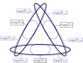
Figure 1: Dividing the supports of local functionals helps with defining $E_{n}^{0}$. In the picture $\mathrm{supp}(F_{1}\otimes F_{2}\otimes F_{3})\cap\mathrm{Diag}(\mathbb{E}^{3})=\emptyset$ but there is no index set $I\subset\left\{1,2,3\right\}$ such that $\mathrm{supp}(F_{1}\otimes F_{2}\otimes F_{3})\subset U_{I}$. However, for any three of the functionals of smaller support such a neighborhood can always be found, $\forall\left(i,j,k\right)$: $\mathrm{supp}(F_{1,i}\otimes F_{2,j}\otimes F_{3,k})\subset U_{I_{\left(i,j,k\right)}}$.

Up to here we have constructed the $n$-fold Euclidean time-ordered products ${E_{n}^{0}(\sum F_{1}\otimes\cdots\otimes F_{n})}$ up to the thin diagonal, under the assumption that the maps $E_{k}$ where already defined on the whole space $\mathbb{E}^{k}$ for all $k<n$. So what remains to be done, is to prove that for each $n\in\mathbb{N}$ the map $E_{n}^{0}$ can be extended to the whole space $\mathbb{E}^{n}$.

IV.2 Extension to the whole space

In their original work (EG, 73), Epstein and Glaser reduce the problem of extending the algebra-valued distributions $T(\mathscr{L}(x_{1})\dots\mathscr{L}(x_{q}))$ (adapting to their notation here) to an extension problem for scalar distributions by expanding the $n$-fold time-ordered product in terms of Wick products of the fields (cf. formulas (42)/(43) loc. cit.). We will show in this section that, using the tools of (BDF, 09), an analogous expansion can be done in the Euclidean framework. The fact that we regard local functionals is essential.

IV.2.1 Expansion Formula of Epstein-Glaser in (Euclidean) pAQFT

The definition of local functionals (Def. II.2) implies that the integral kernel of the $n^{\mathrm{th}}$ functional derivative of any $F\in\mathcal{F}_{\mathrm{loc}}(\mathbb{E})$ can be written as (cf. (BF, 00))

$$F^{\left(n\right)}(\varphi)(x_{1},\dots,x_{n})=\sum_{k}f_{\varphi}^{n,k}(x)\,p_{k}(\partial_{\bm{r}})\,\delta(\bm{r})\,,\quad f_{\varphi}^{n,k}\in\mathscr{D}(\mathrm{Diag}(\mathbb{E}^{n}))\cong\mathscr{D}(\mathbb{E})$$ (23)

where $x=\frac{1}{n}\sum_{i=1}^{n}x_{i}$ is the “center of mass”-coordinate, $\bm{r}=\left(r_{1},\dots,r_{n-1}\right)$ are relative coordinates and $\left(p_{k}\right)_{k\in\mathbb{N}}$ is a basis of homogeneous, symmetric polynomials in $\left(n-1\right)$ variables. Equation (23) is equivalent to saying that the functional derivatives, $F^{\left(n\right)}(\varphi)$, can be restricted to surfaces which are transversal to the thin diagonal $\mathrm{Diag}(\mathbb{E}^{n})$, which is implied by the second condition [LF-2] of Def. II.2 (cf. (Hör, 03, Cor. 8.2.7), (BF, 00, Lem. 6.1)). By using (23) we find a compact formula for the Taylor expansion up to order $N$ of a local functional at some reference field configuration $\varphi_{0}$:

$$F_{\varphi_{0}}^{\left[N\right]}(\varphi) =\sum_{n=0}^{N}\frac{1}{n!}\left\langle F^{\left(n\right)}(\varphi_{0}),\left(\varphi-\varphi_{0}\right)^{\otimes n}\right\rangle$$

$$=\sum_{n=0}^{N}\sum_{k}\left\langle f_{\varphi_{0}}^{n,k}(x),\left\langle\delta(\bm{r}),p_{k}(-\partial_{\bm{r}})\frac{\left(\varphi-\varphi_{0}\right)^{\otimes n}(x,\bm{r})}{n!}\right\rangle\right\rangle$$

$$=\sum_{n=0}^{N}\sum_{k}\left\langle f_{\varphi_{0}}^{n,k}(x),A_{\varphi-\varphi_{0}}^{n,k}(x)\right\rangle\,,$$ (24)

where we introduced the so-called balanced fields (cf. (BOR, 02))

$$A_{\varphi-\varphi_{0}}^{n,k}(x)=\left\langle\delta(\bm{r}),p_{k}(-\partial_{\bm{r}})\frac{\left(\varphi-\varphi_{0}\right)^{\otimes n}(x,\bm{r})}{n!}\right\rangle\,.$$

Following (BDF, 09) we impose two further conditions on the Euclidean $S$-matrix

$$S_{\mathrm{E}}(F):=\exp_{\cdot_{\mathrm{E}}}(F)\equiv\sum_{n=0}^{\infty}\frac{1}{n!}E_{n}(F^{\otimes n})\,.$$ (25)

Let $F\in\mathcal{F}_{\mathrm{loc}}(\mathbb{E})$. The first condition, called $\varphi$-locality, states that the $S$-matrix $S_{\mathrm{E}}(F)(\varphi_{0})$ at a given field configuration $\varphi_{0}$ should depend only on the Taylor expansion of $F$ around $\varphi_{0}$.

Condition 2 ($\varphi$-locality).

$S_{\mathrm{E}}(F)(\varphi_{0})=S_{\mathrm{E}}(F_{\varphi_{0}}^{\left[N\right]})(\varphi_{0})+\mathcal{O}(\hbar^{N+1})$.

This condition makes it possible to treat not only polynomial, but also more general functions of the fields as interaction functionals in pAQFT. Since the $S$-matrix in perturbation theory is defined in terms of a formal power series in $\hbar$, according to Condition 2 $S_{\mathrm{E}}(F)(\varphi_{0})$ is (up to the renormalization freedom) fully determined by the Taylor expansion of $F$ around $\varphi_{0}$, because the additional terms are required to be of sufficiently high order in $\hbar$. Non-polynomial interactions where excluded in the original treatment by Epstein and Glaser. However, their consistent incorporation in the pertubative treatment of QFT is desireable not only from the viewpoint of non-polynomial models like, for instance, the Sine-Gordon model. They also seem to be necessary in a perturbative treatment of super-symmetric extensions of the standard model. Observe, however, that Condition 2 is a condition within perturbation theory, which aims at a consistent treatment of the topic, rather than an extension to the non-perturbative regime.

The second condition, field independence, states that $S$ should only depend implicitly (i.e. via the interaction) on the field configuration $\varphi$, which makes the chain rule easily applicable:

Condition 3 (Field independence).

$\forall g\in\mathscr{E}(\mathbb{E})$: $\left\langle\frac{\delta S_{\mathrm{E}}(F)}{\delta\varphi},g\right\rangle=S_{\mathrm{E}}^{\left(1\right)}(F)\left\langle\frac{\delta F}{\delta\varphi},g~\right\rangle$.

Using Conditions 2 and 3 one can consistently insert the approximation (24) for $F$ into (25). This, as shown below, reduces the extension problem of the functionals $E_{n}^{0}$ to that of certain scalar coefficients in the “Wick expansion” of $E_{n}(F^{\otimes n})$,

$$E_{n}(F^{\otimes n})(\varphi) =E_{n}(F_{\varphi_{0}}^{\left[N\right]}\otimes\cdots\otimes F_{\varphi_{0}}^{\left[N\right]})(\varphi)+\mathcal{O}\left(\hbar^{n\left(N+1\right)}\right)$$

$$=\sum_{l_{j},k_{j}}E_{n}(\left\langle f_{\varphi_{0}}^{l_{1},k_{1}}(x_{1}),A_{\varphi-\varphi_{0}}^{l_{1},k_{1}}(x_{1})\right\rangle\otimes\cdots\otimes\left\langle f_{\varphi_{0}}^{l_{n},k_{n}}(x_{n}),A_{\varphi-\varphi_{0}}^{l_{n},k_{n}}(x_{n})\right\rangle)$$

$$=\sum_{l_{j},k_{j}}\int dx_{1}\cdots dx_{n}\,\prod_{j=0}^{n}f_{\varphi_{0}}^{l_{j},k_{j}}(x_{j})\,E_{n}(A_{\varphi-\varphi_{0}}^{l_{1},k_{1}}(x_{1})\otimes\cdots\otimes A_{\varphi-\varphi_{0}}^{l_{n},k_{n}}(x_{n}))\,.$$

Setting $\varphi=\varphi_{0}$ and defining the scalar distributions

$$t^{l,k}(x_{1},\dots,x_{n}):=E_{n}(A_{\varphi-\varphi_{0}}^{l_{1},k_{1}}(x_{1})\otimes\cdots\otimes A_{\varphi-\varphi_{0}}^{l_{n},k_{n}}(x_{n}))\bigg{|}_{\varphi=\varphi_{0}}\,,\quad l,k\in\mathbb{N}^{n}\,,$$ (26)

we arrive at

$$E_{n}(F^{\otimes n})(\varphi_{0})=\sum_{l_{j},k_{j}}\int dx_{1}\cdots dx_{n}\,\prod_{j=0}^{n}f_{\varphi_{0}}^{l_{j},k_{j}}(x_{j})\,t^{l,k}(x_{1},\dots,x_{n})\,.$$ (27)

Hence the problem of defining the coefficients of the $S$-matrix, $E_{n}(F^{\otimes n})(\varphi_{0})$, for local interactions $F\in\mathcal{F}_{\mathrm{loc}}(\mathbb{E})$ is reduced to extending the coefficients $t^{l,k}$ (26). These are scalar distributions, which in general are well-defined up to the thin diagonal. Observe however, that they only depend on differences of the variables $\left\{x_{1},\dots,x_{n}\right\}$, since the fundamental solution $P(x-y)$ with respect to which the Euclidean time-ordered products $E_{n}$ were defined depend only on relative distances. Hence in flat Euclidean space the distributions $t^{l,k}$ are translation invariant (along diagonal directions), i.e. under transformations $\left(x_{1},\dots,x_{n}\right)\mapsto\left(x_{1}+a,\dots,x_{n}+a\right)$. Consequently, for the extension to the thin diagonal it suffices to define them at the origin.

Example IV.2.

To illustrate this procedure in a graphical setting let us regard the following example

$$\begin{array}[]{c}\\ \mbox{ \fmfgraph*(40,30) \fmfbottom{g,h} \fmftop{f} \fmfdot{f,g,h} \fmflabel{$F^{(5)}$}{f} \fmflabel{$G^{(4)}$}{g} \fmflabel{$H^{(3)}$}{h} \fmf{plain,right=.3}{f,g} \fmf{plain}{f,g} \fmf{plain,left=.3}{f,g} \fmf{plain,right=.3}{g,h} \fmf{plain,right=.3}{h,f} \fmf{plain,left=.3}{h,f} }\\ \\ \end{array}\qquad\qquad\qquad\begin{array}[]{rl}F(\varphi)&=\frac{1}{5!}\int dx\,f(x)\left(\varphi(x)\right)^{5}\,,\\ G(\varphi)&=\frac{1}{4!}\int dx\,g(x)\left(\varphi(x)\right)^{4}\,,\\ H(\varphi)&=\frac{1}{3!}\int dx\,h(x)\left(\varphi(x)\right)^{3}\,,\end{array}$$

with $f,g,h\in\mathscr{D}(\mathbb{E})$ test functions of compact support. The integral kernels of the functional derivatives are given by:

$$\left(F^{\left(5\right)}(\varphi)\right)(x_{1},\dots,x_{5}) =f(x_{1})\,\delta(x_{1}-x_{2})\cdots\delta(x_{4}-x_{5})$$

$$\left(G^{\left(4\right)}(\varphi)\right)(y_{1},\dots,y_{4}) =g(y_{1})\,\delta(y_{1}-y_{2})\cdots\delta(y_{3}-y_{4})$$

$$\left(H^{\left(3\right)}(\varphi)\right)(z_{1},\dots,z_{3}) =h(z_{1})\,\delta(z_{1}-z_{2})\,\delta(z_{2}-z_{3})\,.$$

Hence the corresponding amplitude for the above graph is given by

$$\int dx\,dy\,dz\,\left(P(x-y)\right)^{3}\left(P(x-z)\right)^{2}P(y-z)\,f(x)\,g(y)\,h(z)\,,$$

where in the first induction step the translation invariant distributions $\left(P(x-y)\right)^{3}$ and $\left(P(x-z)\right)^{2}$ have to be extended to the origin, giving renormalized distributions $\left(P(x-y)\right)_{\mathrm{ren}}^{3}$ and $\left(P(x-z)\right)_{\mathrm{ren}}^{2}$, respectively. In the second step the domain of the equally translation invariant distribution

$$t_{0}(x,y,z)=\left(P(x-y)\right)_{\mathrm{ren}}^{3}\left(P(x-z)\right)_{\mathrm{ren}}^{2}P(y-z)$$

has to be extended to give the renormalized amplitude $t_{\mathrm{ren}}$.

IV.2.2 Extension to the origin

The extension problem for scalar distributions, is well understood and can conveniently be discussed in terms of the scaling degree (Ste, 71) of the corresponding distribution.

Definition IV.3 (scaling degree; cf. BF (00)).

Let $\dim(\mathbb{E})=d$ and define

$$\begin{array}[]{rccl}\Lambda:&\mathbb{R}_{+}\times\mathscr{D}(\mathbb{E})&\rightarrow&\mathscr{D}(\mathbb{E})\\ &\left(\lambda,\phi\right)&\mapsto&\phi^{\lambda}:=\lambda^{-d}\phi(\lambda^{-1}\cdot)\end{array}$$

to be the action of the positive real numbers on test functions. This induces, via the pullback, the action on distributions. For $t\in\mathscr{D}^{\prime}(\mathbb{E})$ we have:

$$t_{\lambda}(\phi):=\left(\Lambda^{*}t\right)(\phi)=t(\phi^{\lambda})\,.$$

The scaling degree $\mathrm{sd}(t)$ of a distribution $t$ (with respect to the origin) is defined to be

$$\mathrm{sd}(t):=\inf\left\{\omega^{\prime}\in\mathbb{R}:\,\lim_{\lambda\searrow 0}\lambda^{\omega^{\prime}}t_{\lambda}=0\in\mathscr{D}^{\prime}(\mathbb{E})\right\}\,.$$

The extension of the scalar distributions is governed by the following theorem due to Brunetti and Fredenhagen

Theorem IV.4 (cf. BF (00)).

Let $t_{0}\in\mathscr{D}^{\prime}(\mathbb{R}^{d}\backslash\left\{0\right\})$ have scaling degree $\mathrm{sd}(t_{0})$ with respect to the origin. Let

• $\mathrm{sd}(t_{0})<d$. Then there exists a unique extension $t\in\mathscr{D}^{\prime}(\mathbb{R}^{d})$ of $t_{0}$, i.e. $t(f)=t_{0}(f)$ for all $f\in\mathscr{D}(\mathbb{R}^{d}\backslash\left\{0\right\})$, which has the same scaling degree, $\mathrm{sd}(t)=\mathrm{sd}(t_{0})$.

• $d\leq\mathrm{sd}(t_{0})<\infty$. Then there exist several extensions $t\in\mathscr{D}^{\prime}(\mathbb{R}^{d})$ with $\mathrm{sd}(t)=\mathrm{sd}(t_{0})$, which are uniquely determined by their values on a finite set of test functions.

The freedom in the possible extensions is described by the Stückelberg-Petermann renormalization group, see (BDF, 09) for a thorough discussion of the topic. According to the theorem, given a particular extension $t_{p}$, the most general solution for the extension $t$ of $t_{0}$ reads (cf. (DF, 04))

$$t=t_{p}+\sum_{\left|a\right|\leq\rho(t_{0})}C_{a}\partial^{a}\delta$$ (28)

where $\rho(t_{0}):=\mathrm{sd}(t_{0})-d$ denotes the degree of divergence of $t_{0}$, $a\in\mathbb{N}^{d}$ is a multiindex and $C_{a}\in\mathbb{C}$. Hence the freedom in the choice of an extension $t$ is governed by the scaling degree of $t_{0}$.

Observe, however, that the existence of a renormalized time-ordered product $E_{n}$, given by an extension (28), does not imply that the underlying theory is renormalizable in the sense of power counting. For the sake of readability we quote here the classification of renormalizable theories as it was given by Epstein and Glaser (EG, 73). Given an extension of $E_{n}$ of $E_{n}^{0}$ exists for all orders $n$ of perturbation theory. A theory is called renormalizable, if there is a (finite) upper bound for the degree of divergence of the $n$-fold time-ordered product, $\rho(t_{0}^{n})$, which does not depend on the order $n$ of perturbation theory. The theory is called unrenormalizable, if there is no such bound and it is called superrenormalizable, if there is a certain order $n_{0}$ above which the degree of divergence is negative, i.e. the extensions $E_{n}$ are unique for $n>n_{0}$.

This closes the Euclidean version of the Epstein-Glaser induction and at the same time shows that this induction is completely performable without reference to the star-product structure of Minkowskian pQFT.

V Conclusion

We have shown that the construction of Epstein and Glaser can be adapted to the Euclidean case. On the one hand side, as asserted in the introduction this shows that the construction of Epstein and Glaser can generally be performed without the notion of a star-product. On the other hand the formalism introduced here gives strong tools for the investigation of the local properties of Euclidean QFT. Particularly interesting is the investigation of the relation to other approaches to renormalization, like for instance the BPHZ renormalization scheme. New results in this direction have recently been gained by an investigation of certain examples in momentum space (FHS, 09).

In principle it is possible to get back non-local objects like the analytic Schwinger functions of EQFT from the formalism introduced above. As in the Minkowskian setting of Algebraic Quantum Field Theory one gets back the correlation functions by evaluating their corresponding algebraic versions in the vacuum state. In the introduced setting this is given by the evaluation at $\varphi=0$,

$$\omega_{0}:E_{n}(F_{1}\otimes\cdots\otimes F_{n})\mapsto E_{n}(F_{1}\otimes\cdots\otimes F_{n})\big{|}_{\varphi=0}\,.$$

Performing the adiabatic limit, provided it exists, gives back the Schwinger functions of EQFT.

Appendix A The Wave Front Set of the Dirac Delta Distribution

Just as an example for the computation of the wave front set of a given distribution we compute $\mathrm{WF}(\delta(x,y))$. The singular support of $\delta$ is the diagonal $\mathrm{Diag}(\mathbb{E}^{2})\equiv\left\{\left(x,x\right)\in\mathbb{E}^{2}\right\}$. Following the definition (Hör, 03, Def. 8.1.2) we are interested in the directions $\left(k,k^{\prime}\right)\in T_{\left(x,x\right)}^{*}\mathbb{E}^{2}$ in which the Fourier transform of $\delta$, $\mathrm{FT}(\delta)\equiv\hat{\delta}$, does not decrease rapidly.

$$\hat{\delta}(k,k^{\prime}) =\frac{1}{\left(2\pi\right)^{n}}\int dx\,dy\,e^{-i\left\langle k,x\right\rangle}e^{-i\left\langle k^{\prime},y\right\rangle}\delta(x,y)$$

$$=\frac{1}{\left(2\pi\right)^{n}}\int dx\,e^{-i\left\langle k+k^{\prime},x\right\rangle}=\delta(k+k^{\prime})$$

where one can use Fourier’s inversion formula to show the last equality. Hence the Fouriertransform of $\delta(x,y)$ is rapidly decreasing in all directions except $\left\{\left(k,k^{\prime}\right)\in T_{\left(x,x\right)}^{*}\mathbb{E}^{2}:k+k^{\prime}=0\right\}$. The wave front set of $\delta$ is therefore given by

$$\mathrm{WF}(\delta)=\left\{\left(x,k;x,k^{\prime}\right)\in T^{*}\mathbb{E}^{2}:\,k+k^{\prime}=0\right\}\,.$$

Appendix B Combinatorics: Graphs and Tadpoles

Graphs

As is well known, the symmetry of the time-ordered product is conveniently accounted for by writing its terms as (sums of) graphs. Using Cauchy’s product formula and the Leibniz rule one derives from the formal power series (7) the following expression for the threefold Euclidean time-ordered product, whose addends have a direct interpretation in terms of graphs,

$$F\cdot_{\mathrm{E}}G\cdot_{\mathrm{E}}H \hskip 42.67912pt=\sum_{n=0}^{\infty}\frac{\hbar^{n}}{n!}\sum_{m=k}^{n}\sum_{k=0}^{m}{n\choose m}{m\choose k}\left\langle F^{\left(k+m-k\right)}G_{\left(k\right)}^{\left(n-m\right)}H_{\left(n-m\right)\left(m-k\right)}\right\rangle$$

$$=FGH+\hbar\left(\left\langle FG^{\left(1\right)}H_{\left(1\right)}\right\rangle+\left\langle F^{\left(1\right)}GH_{\left(1\right)}\right\rangle+\left\langle F^{\left(1\right)}G_{\left(1\right)}H\right\rangle\right)$$

$$\quad+\hbar^{2}\left(\frac{1}{2}\left\langle FG^{\left(2\right)}H_{\left(2\right)}\right\rangle+\left\langle F^{\left(1\right)}G^{\left(1\right)}H_{\left(1\right)\left(1\right)}\right\rangle+\left\langle F^{\left(1\right)}G_{\left(1\right)}^{\left(1\right)}H_{\left(1\right)}\right\rangle\right.$$

$$\quad\qquad\qquad\qquad\qquad+\left.\frac{1}{2}\left\langle F^{\left(2\right)}GH_{\left(2\right)}\right\rangle+\left\langle F^{\left(2\right)}G_{\left(1\right)}H_{\left(1\right)}\right\rangle+\frac{1}{2}\left\langle F^{\left(2\right)}G_{\left(2\right)}H\right\rangle\right)$$

$$\quad+\cdots$$

$$=\mbox{ \fmfgraph(20,15) \fmfbottom{g,h} \fmftop{f} \fmfdot{f,g,h} }+\hbar\left(\mbox{ \fmfgraph(20,15) \fmfbottom{g,h} \fmftop{f} \fmfdot{f,g,h} \fmf{plain}{g,h} }+\mbox{ \fmfgraph(20,15) \fmfbottom{g,h} \fmftop{f} \fmfdot{f,g,h} \fmf{plain}{f,h} }+\mbox{ \fmfgraph(20,15) \fmfbottom{g,h} \fmftop{f} \fmfdot{f,g,h} \fmf{plain}{f,g} }\right)$$

$$\quad+\hbar^{2}\left(\frac{1}{2}\,\mbox{ \fmfgraph(20,15) \fmfbottom{g,h} \fmftop{f} \fmfdot{f,g,h} \fmf{plain,right=.5}{g,h} \fmf{plain,left=.5}{g,h} }+\mbox{ \fmfgraph(20,15) \fmfbottom{g,h} \fmftop{f} \fmfdot{f,g,h} \fmf{plain}{f,h} \fmf{plain}{g,h} }+\mbox{ \fmfgraph(20,15) \fmfbottom{g,h} \fmftop{f} \fmfdot{f,g,h} \fmf{plain}{f,g} \fmf{plain}{g,h} }+\frac{1}{2}\,\mbox{ \fmfgraph(20,15) \fmfbottom{g,h} \fmftop{f} \fmfdot{f,g,h} \fmf{plain,right=.5}{f,h} \fmf{plain,left=.5}{f,h} }+\mbox{ \fmfgraph(20,15) \fmfbottom{g,h} \fmftop{f} \fmfdot{f,g,h} \fmf{plain}{f,g} \fmf{plain}{f,h} }+\frac{1}{2}\,\mbox{ \fmfgraph(20,15) \fmfbottom{g,h} \fmftop{f} \fmfdot{f,g,h} \fmf{plain,right=.5}{f,g} \fmf{plain,left=.5}{f,g} }\right)+\cdots$$

The symmetry factor $\mathrm{Sym}(\gamma)^{-1}=\frac{1}{n!}{n\choose m}{m\choose k}=\frac{1}{\left(n-m\right)!k!\left(m-k\right)!}$ of a given term is reflected in the graph as (the reciprocal of) the product of the number of possible permutations of edges which join the same vertices. This is what remains of the symmetry of the functional derivatives after convolution with the fundamental solution $P$. The interpretation in terms of graphs gives a straight-forward generalization to $n$-fold products:

$$E_{n}(F_{1}\otimes\cdots\otimes F_{n})=\sum_{l=0}^{\infty}\hbar^{l}\sum_{\gamma\in\Gamma(n,l)}\frac{1}{\mathrm{Sym}(\gamma)}\,\gamma\,,$$

where $\Gamma(n,l)$ is the set of graphs with $n$ vertices and $l$ edges, in which each edge $e$ joins two different points, $\mathfrak{s}(e)\neq\mathfrak{r}(e)$ (no tadpoles). The graph with the interactions $\left\{F_{1},\dots,F_{n}\right\}$ at $n$ vertices and $l_{i,j}$ edges between $F_{i}$ and $F_{j}$ corresponds to the term:

$$\left\langle\left(F_{1}\right)^{\left(l_{1,2}+l_{1,3}+\cdots+l_{1,n}\right)}\cdots\left(F_{k}\right)_{\left(l_{1,k}\right)\cdots\left(l_{k-1,k}\right)}^{\left(l_{k,k+1}+\cdots+l_{k,n}\right)}\cdots\left(F_{n}\right)_{\left(l_{1,n}\right)\cdots\left(l_{n-1,n}\right)}\right\rangle\,.$$

Notice that both the upper and the lower indices add up to the total number $L$ of edges in the graph,

$$\sum_{i=1}^{n-1}\sum_{j=i+1}^{n}l_{i,j}=\sum_{j=2}^{n}\sum_{i=1}^{j-1}l_{i,j}=\sum_{i<j}l_{i,j}=L\,.$$

Tadpoles

As asserted in the main part of the article, we want to prove here, that there are no tadpole terms, i.e. graphs with at least one line connecting a vertex with itself, in the graph-expansion of $F\cdot_{\mathrm{E}}G$ as defined in (6). By doing so, we give the justification for formula (7).

Proposition B.1.

There are no tadpole terms contributing to ${F\cdot_{\mathrm{E}}G:=}$ ${T_{\mathrm{E}}\circ M\circ\left(T_{\mathrm{E}}^{-1}(F)\otimes T_{\mathrm{E}}^{-1}(G)\right)}$, that is:

$$F\cdot_{\mathrm{E}}G=\sum_{n=0}^{\infty}\frac{\hbar^{n}}{n!}\left\langle F^{\left(n\right)}G_{\left(n\right)}\right\rangle\,.$$

Proof.

The Euclidean time ordering operator, as well as the corresponding operator(s) in pAQFT (BDF, 09) are induced by second order functional differential operators, cf. Eq. (5),

$$\Gamma=\frac{1}{2}\int dx\,dy\,P(x,y)\,\frac{\delta^{2}}{\delta\varphi(x)\,\delta\varphi(y)}\,.$$

As differential operators on $\mathcal{F}(\mathbb{E})$ they fulfill the Leibniz rule, which in turn may be written as a co-product rule:

$$\Gamma(F\cdot G)=M\circ\left(\Delta\Gamma\right)(F\otimes G)\,,\quad\Delta\Gamma=\Gamma\otimes 1+1\otimes\Gamma+\Gamma^{\prime},$$

where

$$\Gamma^{\prime}(F\otimes G)=\int dx\,dy\,P(x,y)\frac{\delta F}{\delta\varphi(x)}\otimes\frac{\delta G}{\delta\varphi(y)}\,.$$

The time-ordered product hence is given by, cf. Eq. (6),

$$F\cdot_{\mathrm{E}}G=e^{\hbar\Gamma}\circ M\circ\left(e^{-\hbar\Gamma}F\otimes e^{-\hbar\Gamma}G\right)\,.$$

Applying the Leibniz rule and using the functional identity for the exponential ($e^{A}e^{B}=e^{A+B}$), which holds due to commutativity and associativity of the product of differential operators, leads to:

$$F\cdot_{\mathrm{E}}G =M\circ e^{\hbar\Delta\Gamma}\circ\left(e^{-\hbar\Gamma}F\otimes e^{-\hbar\Gamma}G\right)$$

$$=M\circ e^{\hbar\Gamma^{\prime}}\left(e^{\hbar\Gamma}e^{-\hbar\Gamma}F\otimes e^{\hbar\Gamma}e^{-\hbar\Gamma}G\right)$$

$$=M\circ e^{\hbar\Gamma^{\prime}}\left(F\otimes G\right)\,.$$

Hence the result stated before:

$$F\cdot_{\mathrm{E}}G=\sum_{n=0}^{\infty}\frac{\hbar^{n}}{n!}\left\langle F^{\left(n\right)},P^{\otimes n}G^{\left(n\right)}\right\rangle\,.$$

∎

Appendix C Local Functionals

The definition of a local functional in (BDF, 09) differs from the one given in this article. Hence, in order to be able to apply their results on local functionals in our context, we have to make sure that the functionals fulfilling the conditions of Definition II.2 are a subset of the set of local functionals in the sense of (BDF, 09, Section 3.2). For this it suffices to show that the support property [LF-1] implies the additivity condition of (BDF, 09). Together with Lemma 3.1 of (BDF, 09) this proves equivalence of both definitions. The argument is taken from (BFR, 09).

Proof.

Let $F$ be a smooth functional fulfilling

$$\frac{\delta^{2}F}{\delta\varphi(x)\delta\varphi(y)}=0\qquad\mbox{for}\,x\neq y\,,$$ (29)

we have to show that

$$\mathrm{supp}(\varphi)\cap\mathrm{supp}(\chi)=\emptyset\quad\mbox{implies}\quad\forall\psi:\;F(\varphi+\psi+\chi)=F(\varphi+\psi)-F(\chi)+F(\psi+\varphi)\,.$$ (30)

We have $\forall\psi$:

$$\frac{\partial^{2}}{\partial\lambda\,\partial\mu}F(\lambda\varphi+\psi+\mu\chi)=\int dx\,dy\,F^{\left(2\right)}(\lambda\varphi+\psi+\mu\chi)(x,y)\,\varphi(x)\,\chi(y)\,,$$ (31)

where due to (29) the domain of integration can be restricted to the diagonal $\left\{\left(x,y\right):x=y\right\}$. And since $\forall x$: $\varphi(x)\chi(x)=0$ due to the assumption in (30), we have that the integral on the right hand side of (31) vanishes, i.e.

$$\frac{\partial^{2}}{\partial\lambda\,\partial\mu}F(\lambda\varphi+\psi+\mu\chi)\equiv 0\,.$$

Integration with respect to $\lambda$ gives

$$\frac{\partial}{\partial\mu}F(\varphi+\psi+\mu\chi) =\int_{0}^{1}d\lambda\,\frac{\partial^{2}}{\partial\lambda\,\partial\mu}F(\lambda\varphi+\psi+\mu\chi)+\frac{\partial}{\partial\mu}F(\psi+\mu\chi)$$

$$=\frac{\partial}{\partial\mu}F(\psi+\mu\chi)\,,$$

and integrating another time with respect to $\mu$ gives the desired result:

$$F(\varphi+\psi+\chi) =F(\varphi+\psi)+\int_{0}^{1}d\mu\,\frac{\partial}{\partial\mu}F(\psi+\mu\chi)$$

$$=F(\varphi+\psi)-F(\psi)+F(\psi+\chi)\,.$$

∎

References

- BDF (09) R. Brunetti, M. Dütsch, and K. Fredenhagen. Perturbative Algebraic Quantum Field Theory and the Renormalization Groups. 2009. arXiv:0901.2038.
- BF (00) R. Brunetti and K. Fredenhagen. Microlocal Analysis and Interacting Quantum Field Theories: Renormalization on Physical Backgrounds. Commun. Math. Phys., 208(3):623–661, 2000.
- BFR (09) R. Brunetti, K. Fredenhagen, and P. Lauridsen Ribeiro. 2009. forthcoming paper.
- BG (96) C. G. Bollini and J. J. Giambiagi. Dimensional regularization in configuration space. Phys. Rev. D, 53(10):5761, May 1996.
- BOR (02) D. Buchholz, I. Ojima, and H. Roos. Thermodynamic Properties of Non-Equilibrium States in Quantum Field Theory. Ann. Physics, 297(2):219–242, 2002.
- BP (57) N. N. Bogoliubow and O. S. Parasiuk. Über die Multiplikation der Kausalfunktionen in der Quantentheorie der Felder. Acta Mathematica, 97(1-4):227–266, 1957.
- Bro (09) C. Brouder. Hopf algebraic structures of quantum field and many-body theories. Lecture given at the ACQFT conference in Cargèse, Corsica, 2009. http://www.lmcp.jussieu.fr/~brouder/talk.html.
- BS (59) N. N. Bogoliubov and D. V. Shirkov. Introduction to the Theory of Quantized Fields. Interscience Publishers, 1959.
- DF (01) M. Dütsch and K. Fredenhagen. Perturbative Algebraic Field Theory, and Deformation Quantization. In R. Longo, editor, Mathematical Physics in Mathematics and Physics: Quantum and Operator Algebraic Aspects, volume 30 of Fields Institute Communications, Providence, RI, 2001. AMS. Proceedings of the conference held in Siena on June 20-24, 2000; arXiv:hep-th/0101079.
- DF (04) M. Dütsch and K. Fredenhagen. Causal Perturbation Theory in Terms of Retarded Products, and a Proof of the Action Ward Identity. Rev. Math. Phys., 16(10):1291–1348, 2004.
- EE (79) J. P. Eckmann and H. Epstein. Time-ordered products and Schwinger functions. Commun. Math. Phys., 64(2):95–130, June 1979.
- EG (73) H. Epstein and V. Glaser. The Role of Locality in Perturbation Theory. Ann. Inst. Henri Poincaré, 19(3):211–295, 1973.
- FHS (09) S. Falk, R. Häußling, and F. Scheck. Renormalization in Quantum Field Theory: An Improved Rigorous Method. 2009. arXiv:0901.2252.
- GS (08) D.R. Grigore and G. Scharf. No-Go Result for Supersymmetric Gauge Theories in the Causal Approach. Annalen der Physik, 17(11):864–880, 2008.
- Hep (66) K. Hepp. Proof of the Bogoliubov-Parasiuk Theorem on Renormalization. Commun. Math. Phys., 2(4):301–326, 1966.
- HH (02) A. C. Hirshfeld and P. Henselder. Star Products and Perturbative Quantum Field Theory. Ann. Physics, 298(2):382–393, 2002.
- Hör (03) L. Hörmander. The Analysis of Linear Partial Differential Operators I: Distribution Theory and Fourier Analysis. Classics in Mathematics. Springer, 2003.
- HW (01) S. Hollands and R. M. Wald. Local Wick Polynomials and Time Ordered Products of Quantum Fields in Curved Spacetime. Commun. Math. Phys., 223(2):289–326, 2001.
- OS (73) K. Osterwalder and R. Schrader. Axioms for Euclidean Green’s functions. Commun. Math. Phys., 31(2):83–112, 1973.
- OS (75) K. Osterwalder and R. Schrader. Axioms for Euclidean Green’s functions II. Commun. Math. Phys., 42(3):281–305, 1975.
- Roe (94) G. Roepstorff. Path Integral Approach to Quantum Physics. Springer, 1994.
- RS (80) M. Reed and B. Simon. Functional Analysis, volume 1 of Methods of Modern Mathematical Physics. Academic Press, 1980.
- Sal (99) M. Salmhofer. Renormalization - An Introduction. Springer, 1999.
- Sch (59) J. Schwinger. Euclidean Quantum Electrodynamics. Phys. Rev., 115:721–731, 1959.
- Sib (08) K. Sibold. Comment to ‘No-Go Result for Supersymmetric Gauge Theories in the Causal Approach’, by D. R. Grigore and G. Scharf (previous article: Ann. Phys. (Berlin) 17, 864 (2008)). Annalen der Physik, 17(11):881–884, 2008.
- SR (50) E. C. G. Stückelberg and D. Rivier. A propos des divergences en théorie des champs quantifiés. Helv. Phys. Acta, 23 (Suppl. III):236–239, 1950.
- Ste (71) O. Steinmann. Perturbation Expansions in Axiomatic Field Theory, volume 11 of Lecture Notes in Physics. Springer, Berlin and Heidelberg, 1971.
- Sto (06) R. Stora. Causalité et Groupes de Renormalisation Perturbatifs. unpublished lecture notes, Ecole de Physique Théorique de Jijel, Algérie, 2006.
- SW (64) R. F. Streater and A. S. Wightman. PCT, Spin and Statistics, and all that. W.A. Benjamin, Inc., Amsterdam and New York, 1964.
- Sym (69) K. Symanzik. Euclidean Quantum Field Theory. In R. Jost, editor, Local Quantum Theory, number Course XLV in Proceedings of the International School of Physics ’Enrico Fermi’, pages 152–226, New York and London, 1969. Academic Press.
- Zim (69) W. Zimmermann. Convergence of Bogoliubov’s Method of Renormalization in Momentum Space. Commun. Math. Phys., 15(3):208–234, 1969.