Quantum algorithm for the Laughlin wave function

Abstract

We construct a quantum algorithm that creates the Laughlin state for an arbitrary number of particles $n$ in the case of filling fraction one. This quantum circuit is efficient since it only uses $n(n-1)/2$ local qudit gates and its depth scales as $2n-3$. We further prove the optimality of the circuit using permutation theory arguments and we compute exactly how entanglement develops along the action of each gate. Finally, we discuss its experimental feasibility decomposing the qudits and the gates in terms of qubits and two qubit-gates as well as the generalization to arbitrary filling fraction.

One of the most important goals in the field of quantum computation is to achieve a faithful and efficient simulation of relevant quantum systems. Feynman first suggested F82 ; NC00 the possibility of emulating a quantum system by means of other specially designed and controlled quantum systems. Nowadays, ultra-cold atoms in optical lattices are producing the first quantum simulators LSADSS07-BDZ08 and many theoretical proposals have been already presented in order to approximately simulate strongly correlated systems PPC ; HSDL07 ; BHHFZ05 ; PB08 ; MBZ06 ; DDL03 .

A more ambitious goal consists in finding the exact quantum circuit that underlies the physics of a given quantum system. Rather than searching for an analogical simulation, such an exact quantum circuit would fully reproduce the properties of the system under investigation without any approximation and for any experimental value of the parameters in the theory. It is particularly interesting to device new quantum algorithms for strongly correlated quantum systems of few particles. These could become the first non-trivial uses of a small size quantum computer. It is worth recalling that strong correlations are tantamount to a large amount of entanglement in the quantum state and this, in turn, implies that the system is hard to be simulated numerically G03 .

An exact quantum circuit would start from a simple product unentangled state and would create faithfully any desired state on demand. That is, such a quantum algorithm would diagonalize the dynamics of the target system. At present, very few cases are under control BS08 ; VCL08 . In Ref. VCL08 , the underlying quantum circuit that reproduces the physics of the thoroughly studied XY Hamiltonian was obtained. The philosophy inspiring that circuit was to follow the steps of the analytical solution of that integrable model. It is not obvious how to design a quantum simulator for non-integrable systems. Here, we shall present a quantum circuit that allows the controlled construction of a particular case of the Laughlin wave function. Thus, the quantum algorithm we are putting forward will not produce the complete dynamics of a Hamiltonian but rather a specific state. That is, our quantum circuit will transform a trivial product state into a Laughlin state with filling fraction one by means of a finite amount of local two-body quantum gates.

Let us start by recalling the Laughlin L83 wave function for filling fraction $\nu=1/m$, which corresponds to

$$\Psi_{L}^{(m)}(z_{1},\ldots,z_{n})\sim\prod_{i<j}(z_{i}-z_{j})^{m}e^{-\sum_{i=1}^{N}|z_{i}|^{2}/2}\ ,$$ (1)

where $z_{j}=x_{j}+\textrm{i}y_{j},j=1,\ldots,n$ stands for the position of the $j$-th particle. This state was postulated by Laughlin as the ground state of the fractional quantum Hall effect (FQHE) Tsui82 . From the quantum information point of view, the Laughlin state exhibits a considerable von Neumann entropy between for any of its possible partitions ILO07 . It is, thus, classically hard to simulate such a wave function making it an ideal problem for a quantum computer.

We shall construct the Laughlin state using a quantum system that consists of a chain of $n$ qudits ($d$-dimensional Hilbert spaces). In our case, that is $m=1$, the dimension of the qudits is needed to be $d=n$. Let us proceed to construct the quantum circuit by first considering the case of $n=2$ particles, then $n=3$ and, finally, the general case.

The Laughlin state can be written in terms of the single particle angular momentum eigenstates, also called Fock-Darwin states $\varphi_{l}(z)=\langle{z}|l\rangle=z^{l}\exp(-|z|^{2}/2)/\sqrt{\pi l!}$. Then, the $n=2$ Laughlin state reads

$$\Psi_{L}^{(2)}(z_{1},z_{2})=\frac{1}{\sqrt{2}}\left(\varphi_{1}(z_{1})\varphi_{0}(z_{2})-\varphi_{0}(z_{1})\varphi_{1}(z_{2})\right)\ .$$ (2)

Let us note that $\Psi_{L}^{(2)}(z_{1},z_{2})=\langle{z_{1},z_{2}}|\Psi_{2}^{(2)}\rangle$ is simply the projection of the Laughlin state

$$|{\Psi_{L}^{(2)}}\rangle=\frac{1}{\sqrt{2}}\left(|{0,1}\rangle-|{1,0}\rangle\right)\,$$ (3)

in coordinates representation, where particle label is retained in the order of qubits and the angular momentum 0 or 1 is an element of the angular momentum basis.

It is trivial to find a quantum circuit that transforms a product state into the above $n=2$ Laughlin state. Let us first prepare an initial state as $|{\Psi_{0}^{(2)}}\rangle=|{0,1}\rangle$ and perform on it the simple two-qubit gate $U[2]$ as shown in Fig. 1. The exact form of the unitary operator $U[2]$ in the angular momentum basis $\{|{0,0}\rangle,|{0,1}\rangle,|{1,0}\rangle,|{1,1}\rangle\}$ is

$$U[2]=\begin{pmatrix}1&0&0&0\\ 0&\frac{1}{\sqrt{2}}&\frac{1}{\sqrt{2}}&0\\ 0&-\frac{1}{\sqrt{2}}&\frac{1}{\sqrt{2}}&0\\ 0&0&0&1\end{pmatrix}\,.$$ (4)

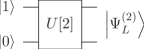
Figure 1: Scheme for the quantum circuit that generates the $n=2$ Laughlin state by acting on the product state $|\Psi_{0}^{(2)}\rangle=|{0,1}\rangle$. Notice that the qubits of the input state are labeled from bottom to top.

Let us now move to the more complicate case of the Laughlin state with three particles, $n=3$. We now need to consider a system of three qutrits $d=n=3$. Following similar steps as we did for $n=2$, we take as initial state $|{\Psi_{0}^{(3)}}\rangle=|{0,1,2}\rangle$, that is, each qutrit is prepared in a different basis element, representing different angular momenta. The aim of the quantum circuit is to antisymmetrize this initial state, since the Laughlin wave function for $m=1$ is simply the Slater determinant of the single particle wave functions

$$\Psi_{L}^{(3)}(z_{1},z_{2},z_{3}) =\langle{z_{1},z_{2},z_{3}}|\Psi_{L}^{(3)}\rangle$$

$$=\frac{1}{\sqrt{6}}\left|\begin{array}[]{ccc}\varphi_{0}(z_{1})&\varphi_{0}(z_{2})&\varphi_{0}(z_{3})\\ \varphi_{1}(z_{1})&\varphi_{1}(z_{2})&\varphi_{1}(z_{3})\\ \varphi_{2}(z_{1})&\varphi_{2}(z_{2})&\varphi_{2}(z_{3})\end{array}\right|\,.$$ (8)

To do this, we define the two-qutrit unitary operators $W_{ij}(p)$ as

$$W_{ij}(p)|{ij}\rangle =\sqrt{p}|{ij}\rangle-\sqrt{1-p}|{ji}\rangle$$

$$W_{ij}(p)|{ji}\rangle =\sqrt{p}|{ji}\rangle+\sqrt{1-p}|{ij}\rangle\,,$$ (9)

for $i<j$, $0\leq p\leq 1$, and $W_{ij}|{kl}\rangle=|{kl}\rangle$ if $(k,l)\neq(i,j)$. We realize that for the case of qubits and $p=1/2$ we recover the gate $U[2]$ of Eq. (4). Let us note that the unitary operator $W_{ij}$ is a linear combination of the identity ($p=1$) and the simple transposition ($p=0$) operators, where a simple transposition is defined as the transposition between two contiguous elements.

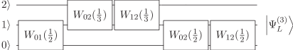
Figure 2: Quantum circuit that produces the $n=3$ Laughlin state acting on a product state $|\Psi_{0}^{(3)}\rangle=|{0,1,2}\rangle$.

The architecture of the quantum circuit that produces the $n=3$ Laughlin state in Eq. (8) by means of the local gates from Eq. (9) is presented in Fig. 2.

So far, we have seen the quantum circuits that produce the Laughlin state for $n=2$ and 3. From these cases, a general scheme emerges that will produce the correct quantum circuit for an arbitrary number of particles. Let us proceed by induction. We will assume that we already know the quantum circuit, $U[n]$, that produces the Laughlin state for $n$ qudits when acting on $|{\Psi_{0}^{(n)}}\rangle=|{0,1,2,\dots,n-1}\rangle$. We now need to complete the circuit to achieve the $n+1$ Laughlin state from the product state $|{\Psi_{0}^{(n+1)}}\rangle=|{0,1,\dots,n-1,n}\rangle$.

The Laughlin state for $n$ qudits has the form

$$|{\Psi_{L}^{(n)}}\rangle=\frac{1}{\sqrt{n!}}\sum_{\mathcal{P}}\textrm{sign}(\mathcal{P})|{a_{1},\ldots,a_{n}}\rangle\,,$$ (10)

where the sum runs over all the possible permutations of the set $\{0,1,\ldots,n-1\}$ and, given a permutation, $a_{k}$ represents its $k$-th element. The relative sign between two permutations corresponds to the parity of the number of transpositions needed to transform one into the other. If we add another qudit, the system is in a product state $|{\Psi_{L}^{(n)}}\rangle|{n}\rangle$. According to Eq. (10), we want to generate a superposition of $(n+1)!$ permutations corresponding to the $n+1$ states of the Laughlin wave function, from the superposition of $n!$ permutations that we already have in the $n$-qudit case.

Let us note that, if we have the set of $n!$ permutations of $n$ elements, we can generate the set of permutations of $n+1$ elements by performing successive simple transpositions between the new element and its preceding neighbour in the sequence $\left(\{a_{1},\ldots,a_{n},n\}\right.$, $\{a_{1},\ldots,n,a_{n}\}$, $\ldots$, $\left.\{n,a_{1},\ldots,a_{n}\}\right)$.

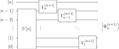
Figure 3: Quantum circuit that produces the Laughlin state for an arbitrary number of wires $(n+1)$ acting on a product state $|{\Psi_{0}^{(n)}}\rangle=|{0,1,2,\cdots,n}\rangle$. Note its recursive structure, $U[n+1]=V_{1}^{[n+1]}V_{2}^{[n+1]}\ldots V_{n}^{[n+1]}U[n]$, where $V$ gates are defined in Eq. (12).

This idea suggests a circuit as the one shown in Fig. 3. In this scheme, the gate $V_{n}^{[n+1]}$ should produce a superposition of all the permutations $|{a_{1},\ldots,a_{n},n}\rangle$ with $|{a_{1},\ldots,n,a_{n}}\rangle$. The gate $V_{n-1}^{[n+1]}$ should do the same task in the next site, that is, should produce a superposition between $|{a_{1},\ldots,a_{n-1},n,a_{n}}\rangle$ and $|{a_{1},\ldots,n,a_{n-1},a_{n}}\rangle$. This scheme works successively till $V_{1}^{[n+1]}$.

This general structure implies that $V_{n}^{[n+1]}$ has to be decomposed in terms of the $W$-gates presented previously,

$$V_{n}^{[n+1]}=W_{0n}(p)W_{1n}(p)\ldots W_{n-1\,n}(p)\,,$$ (11)

where $p$ is a common weight due to the fact that the $0,\ldots,n-1$ states in the Laughlin wave function are indistinguishable. Let us note that all the operators $W_{in}$ in the previous expression commute among themselves and, therefore, the order in which they are applied is irrelevant.

In order to determine the weight $p$ in the $V_{n}^{[n+1]}$ gate, we realize that if all the transpositions only involve the state $n$, the states $|{a_{1},\ldots,a_{n},n}\rangle$ will not be affected by the rest of gates, and they should already have the correct normalization factor $\frac{1}{\sqrt{(n+1)!}}$ after applying $V_{n}^{[n+1]}$. This implies $p=\frac{1}{n+1}$.

We proceed in a similar way to determine the rest of gates, and we obtain

$$V_{k}^{[n+1]}=\prod_{i=0}^{n-1}W_{in}\,,$$ (12)

where, given a $k$, all the $W$ gates have the same weight $\frac{1}{k+1}$ and $k=1\ldots n-1$. Notice that the $W_{ij}$ gates act on states with $i<j$ along the whole circuit and, therefore, they always generate the negative combination $\sqrt{p}|{ij}\rangle-\sqrt{1-p}|{ji}\rangle$. This is the reason why each term of the final state has the appropriate sign, since a minus sign is carried in each transposition.

The above discussion produces our main result, that is, the circuit shown in Fig. 3 that uses the definition of its gates in Eq. (12). Such a quantum circuit will generate the $m=1$ Laughlin wave function for an arbitrary number of qudits. In particular, the quantum circuit corresponding to 5 qudits is presented in Fig. 4.

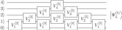
Figure 4: Quantum circuit that produces the Laughlin state of 5 particles acting on a product state $|{01234}\rangle$.

The recursive structure of the circuit (Fig. 3) makes easy to calculate how the number of gates $N(n)$ and the depth $D(n)$ of the circuit scale with the total number of particles $n$. An elementary counting gives the result

$$N(n) =(n-1)+N(n-1)=\frac{n(n-1)}{2}$$

$$D(n) =D(n-1)+2=2n-3,$$ (13)

with $N(2)=1$ and $D(2)=1$. The quantum circuit that delivers the Laughlin state is, thus, efficient since the number of gates scales polynomially. This is a non-trivial result since, in general, an arbitrary unitary transformation requires an exponential number of gates to be performed.

Let us now discuss the optimality of our quantum circuit. As we mentioned previously, a simple transposition, $s_{i}$, is defined as the transposition between two contiguous elements, $i$ and $i+1$. Any permutation can be decomposed in terms of a series of simple transpositions and its minimal decomposition is called the canonical reduced decomposition. There are two particular interesting permutations: (i) the minimum permutation ($0,1,2,\ldots,n-1$) whose canonical reduced decomposition is the identity, and (ii) the maximum permutation ($n-1,n-2,\ldots,0$) whose canonical reduced decomposition reads $s_{1}(s_{2}s_{1})(s_{3}s_{2}s_{1})\ldots(s_{n-1}\ldots s_{1})\,,$ and it is the permutation with the largest number of simple transpositions in its canonical reduced decomposition. Then, a circuit that produces the state corresponding to the maximum permutation needs as many gates as the number of simple transpositions of its canonical reduced decomposition, that is $\frac{n(n-1)}{2}$. The Laughlin state contains this maximum permutation, therefore, its quantum circuit must have, at least, $\frac{n(n-1)}{2}$ gates, that is precisely the number of gates in our proposal.

It is also possible to analyze the way entanglement grows along the circuit. In order to do this, we calculate how much entanglement each gate of the circuit generates, that is, we determine the increase of the von Neumann entropy between the two parts of the system separated by a given gate,

$$\Delta S\left(V_{k}^{[n]}\right)=\log_{2}\left(\frac{n}{n-k}\right)\,.$$ (14)

The von Neumann entropy between $k$ particles and the rest of the system is simply the sum of the contributions of those gates that are in the row which separates the system in $k$ and $n-k$ wires. These gates are $V_{k}^{[n^{\prime}]}$ for $k+1\leq n^{\prime}\leq n$ and the entanglement entropy reads

$$S_{n,k}=\sum_{n^{\prime}=k+1}^{n}\Delta S\left(V_{k}^{[n^{\prime}]}\right)=\log_{2}\binom{n}{k}\,.$$ (15)

This expression recovers in a clean way the same result as the one found in Ref. ILO07 , which was proven exact. Let us also remark that although each single particle is maximally entangled with the rest of the system, a subset of $k\leq n/2$ particles does not saturate the entropy,

$$S_{n,k}\leq k\log_{2}{n}\,.$$ (16)

A experimental realization of our proposal will probably need to work on qubits rather than qudits. It is, then, necessary to find an efficient reduction of our algorithm to qubits. The easiest way to encode a qudit in terms of qubits is the binary basis. Then, an arbitrary single state $|{i}\rangle$ can be decomposed as $|{i}\rangle=|{i_{r}}\rangle\ldots|{i_{2}}\rangle|{i_{1}}\rangle\,,$ where $i=\sum_{k=1}^{r}2^{k-1}i_{k}$, $r\sim\log_{2}n$ is the number of bits needed to represent $n$, and $i_{k}=0,1$ $\forall k=1,\ldots,r$.

Now, we want to find the gates that acting on these qubits implement the $W$ gates. $W_{ij}$ acts non trivially on the space spanned by the computational basis states $|{ij}\rangle\equiv|{i_{r},\ldots,i_{1},j_{r},\ldots,j_{1}}\rangle$ and $|{ji}\rangle\equiv|{j_{r},\ldots,j_{1},i_{r},\ldots,i_{1}}\rangle$, and is the identity for the rest of states. Let us define $\tilde{W}$ as the non trivial $2\times 2$ sub matrix of $W$ that acts on this subspace. According to Eq. (9), $\tilde{W}$ takes the form

$$\tilde{W}\equiv\begin{pmatrix}\sqrt{p}&\sqrt{1-p}\\ -\sqrt{1-p}&\sqrt{p}\end{pmatrix}\,,$$ (17)

and it corresponds to the exponentiation $\tilde{W}=\exp{\left(\textrm{i}\theta\sigma_{y}\right)}$ of the $\sigma_{y}$ Pauli matrix for $p=\cos^{2}\frac{\theta}{2}$. In order to implement an arbitrary $W_{ij}$ gate, we have to follow three steps: (i) first, we compare the binary expressions of $i_{r}\ldots i_{1}j_{r}\ldots j_{1}$ and $j_{r}\ldots j_{1}i_{r}\ldots i_{1}$, and notice which bits are different. Then, we carry out a sequence of binary numbers, starting with $ij$ and concluding with $ji$, such that adjacent members of the list differ in only one bit. These sequences are called Gray codes NC00 . (ii) Next, we implement a quantum circuit performing a series of multi-qubit controlled gates that change the state $ij$ according to the previous sequence. Each multi-qubit gate transforms the corresponding state of the sequence into the next one. These multi-qubits gates are carried out until it only remains a different bit between the last transformed state and $ji$. (iii) At this point, we perform a controlled-$\tilde{W}$ gate, or alternatively its complex conjugate $\tilde{W}^{\dagger}$, taking this different qubit as target. We will apply $\tilde{W}$ or $\tilde{W}^{\dagger}$ depending on the initial state in which the single gate is performed in order to tune the behaviour of $W$ according to its definition in Eq. (9). Finally, the reversed previous sequence of multi-qubit controlled gates is performed.

This abstract construction can be illustrated with the example of the $W_{35}$ gate that acts non-trivially on the states $|{011\ 101}\rangle$ and $|{101\ 011}\rangle$. One possible sequence of Gray codes that connect $011\ 101$ and $101\ 011$ is

$$\begin{array}[]{ccccccc}0&1&1&&1&0&1\\ {\bf 1}&1&1&&1&0&1\\ 1&{\bf 0}&1&&1&0&1\\ 1&0&1&&{\bf 0}&0&1\\ 1&0&1&&0&1&1\,.\end{array}$$ (18)

From this, we can read its corresponding circuit, shown in Fig. 5. Notice that the first three multi-qubit controlled gates transforms $|{011\ 101}\rangle$ into $|{101\ 001}\rangle$. Next, the $\tilde{W}$ gate is applied to the fifth qubit, affecting only the states $|{101\ 001}\rangle$ and $|{101\ 011}\rangle$ due to the conditions on rest of qubits. Finally, we reverse the application of the multi-qubit controlled gates, ensuring that $|{101\ 001}\rangle$ gets swapped back with $|{011\ 101}\rangle$.

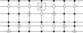
Figure 5: Implementation of the $W_{35}$ gate in terms of multi-qubit control gates. Each of these controlled operations can be decomposed in single qubit and CNOT gates.

It is important to point out that these multi-qubit controlled gates are not two-qubit gates, as, in principle, it would be suited. Nevertheless, it is known that these controlled operations can be performed by means of $O(r)$ single qubit and CNOT gates MMKIW95 ; BBCDMSSSW95 which can be implemented experimentally CZ95 ; CCEHRSZ06 . Thus, if we consider that the number of $W$-gates that we have to perform to implement our proposal for $n$ qudits is $\frac{n(n-1)(2n-1)}{6}$, the number of single qubit and CNOT gates required by our circuit scales as $O\left(n^{3}(\log_{2}n)^{2}\right)$.

There’s a second way of encoding a qudit in the state $|{i}\rangle$, that is, take $n$ qubits, set the $i$-th one to $|{1}\rangle$, and then the rest to $|{0}\rangle$, i. e. $|{i}\rangle=|{0\ldots 010\ldots 0}\rangle$. This unary encoding is less efficient than the previous one, since it requires $n$ qubits compared to the $\log_{2}n$ required before. Nevertheless, it has the advantage that allows us to implement the $W$-gates using less gates. We just follow the previous three steps with the four qubits that have to be affected by the gate, that is, the $i$-th, $j$-th, $(n+i)$-th and $(n+j)$-th. We realize that only 3 different multi controlled gates are required. In this case, then, the number of single qubit and CNOT gates required by our circuit would be $O\left(n^{3}\right)$.

Moreover, let us note that we can transform our antisymmetrization circuit into a symmetrization one by just changing the signs of the definition of the $W$ gates in Eq. (9), i.e. $\sqrt{p}|{ij}\rangle\mp\sqrt{1-p}|{ji}\rangle\ \to\ \sqrt{p}|{ij}\rangle\pm\sqrt{1-p}|{ji}\rangle$. Another possibility of performing the same symmetrization would be to invert the order of the input state of the circuit ($|{n-1,\ldots,0}\rangle$ instead of $|{0,\ldots,n-1}\rangle$) and to apply the gates $W_{n-1-i,n-1-j}$, instead of $W_{ij}$, along the circuit. In both cases, the W gates always act in the positive combination and the final state obtained is fully symmetric in all possible permutations.

Let us conclude with some comments on the generalization of our proposal to other values of $m$. The first observation is that, if $m>1$, the number of states that appear in the superposition of the Laughlin wave function is much larger than the simple permutations of the input single states. The corresponding quantum circuit, therefore, cannot be only composed of $W$-gates. This will increase a lot the degrees of freedom of our elementary gates and, thus, its complexity. Though specific examples for low values of $n$ and $m$ can be found, a general scheme is still missing.

Acknowledgements. Financial support from QAP (EU), ICINN (Spain), FI program and Grup Consolidat (Generalitat de Catalunya), and QOIT Consolider-Ingenio 2010 is acknowledged.

References

- (1) R. Feynman, Internat. J. Theoret. Phys., 21, pp 467-488 (1982).
- (2) M. A. Nielsen, and I. L. Chuang, Quantum Computation and Quantum Information, (Cambridge Univ. Press, Cambridge, England, 2000).
- (3) M. Lewenstein et al. , Adv. in Phys. 56, 243 (2007). I. Bloch, J. Dalibard and W. Zwerger, Rev. Mod. Phys. 80, 885 (2008).
- (4) M. Popp, B. Paredes and J. I. Cirac, Phys. Rev. A 70, 053612 (2004).
- (5) M. Hafezi et al., Phys. Rev. A 76, 023613 (2007).
- (6) H. P. Büchler et al. , Phys. Rev. Lett. 95, 040402 (2005).
- (7) B. Paredes and I. Bloch, cond-mat/0711.3796, (2007).
- (8) A. Micheli, G.K. Brennen and P. Zoller, Nat. Phys. 2, 341 (2006).
- (9) L. M. Duan, E. Demler and M. D. Lukin, Phys. Rev. Lett. 91 090402 (2003).
- (10) G. Vidal, Phys. Rev. Lett. 91 147902 (2003). G. Vidal, Phys. Rev. Lett. 93 040502 (2004).
- (11) G. Benenti and G. Strini, Am. J. Phys. 76 657 (2008).
- (12) F. Vestraete, J. I. Cirac and J. I. Latorre, quant-ph/0804.1888, (2008).
- (13) R. B. Laughlin, Phys. Rev. Lett. 50, 1395 (1983).
- (14) D. C. Tsui, H. L. Stormer and A. C. Gossard, Phys. Rev. Lett. 48 1559 (1982).
- (15) S. Iblisdir, J. I. Latorre and R. Orús, Phys. Rev. Lett. 98 060402 (2007).
- (16) C. Monroe et al. , Phys. Rev. Lett. 75, 4714 (1995).
- (17) A. Barenco et al. , Phys. Rev. A 52, 3457 (1995).
- (18) J. I. Cirac and P. Zoller, Phys. Rev. Lett. 74, 4091 (1995).
- (19) G. Chen et al. , Quantum Computing Devices: Principles, Designs, and Analysis, (CRC Press, 2006).