DESY 09–012
SFB/CPP–09–12
HEPTOOLS 08-230
New results for loop integrals:
AMBRE, CSectors, hexagon

Abstract:

We report on the three Mathematica packages hexagon, CSectors, AMBRE. They are useful for the evaluation of one- and two-loop Feynman integrals with a dependence on several kinematical scales. These integrals are typically needed for LHC and ILC applications, but also for higher order corrections at meson factories. hexagon is a new package for the tensor reduction of one-loop 5-point and 6-point functions with rank $R=3$ and $R=4$, respectively; AMBRE is a tool for derivations of Mellin-Barnes representations; CSectors is an interface for the package sector_decomposition and allows a convenient, direct evaluation of tensor Feynman integrals.

1 Introduction

In recent years, we observe that higher energy, higher luminosity, higher precision, more massive particles at LHC and ILC, but also at low energy meson factories, lead to completely new demands on the efficient evaluation of Feynman diagrams, including:

• need of some 3-point 4-point two-loop diagrams, including double boxes,

• need of many $n$-point one-loop diagrams,

with massive and massless particles participating, leading to complicated many-scale problems.

A few of the approaches to answer the requests will be shortly introduced, concentrating on our own activities and on publicly available packages. They are devoted to the evaluation of $L$-loop $n$-point Feynman integrals of tensor rank $R$, with loop momenta $k_{l}$, with $E$ external legs with momenta $p_{e}$, and with $N$ internal lines with masses $m_{i}$ and propagators $1/D_{i}$:

$$I^{\{\alpha\}} = \frac{e^{L\varepsilon\gamma_{E}}}{(i\pi^{d/2})^{L}}\int\frac{d^{d}k_{1}\ldots d^{d}k_{L}~{}~{}N^{\alpha_{1}\cdots\alpha_{R}}}{D_{1}^{\nu_{1}}\ldots D_{i}^{\nu_{i}}\ldots D_{N}^{\nu_{N}}},$$ (1)

$$D_{i} = \left(q_{i}^{2}-m_{i}^{2}\right)~{}=~{}\left[\sum_{l=1}^{L}c_{i}^{l}k_{l}+\sum_{e=1}^{E}d_{i}^{e}p_{e}\right]^{2}-m_{i}^{2}~{},$$ (2)

where we call $d=4-2\varepsilon$ the generic dimension and $\nu_{i}$ the index of the propagator. The numerator may contain a tensor structure, e.g.:

$$N = 1,~{}~{}~{}k_{1}^{\alpha_{1}}k_{1}^{\beta_{1}},~{}~{}~{}k_{1}^{\alpha_{1}}\cdots k_{R}^{\alpha_{R}}.$$ (3)

There exists no general algorithm for the calculation of arbitrary Feynman integrals, but there exists a rising number of tools, and some of them are publicly available. In the next sections, I will comment on recent developments around three of them.

The Feynman integrals may be evaluated in quite different ways. One may derive for them (systems of coupled) difference or differential equations, or one may seek a (minimal) basis of (scalar) master integrals, and solve only the latter ones, etc. Often the Feynman parameter representation is useful, which replaces the $d$-dimensional momentum integrations by an appropriate number of parameter integrals. Feynman parameters are introduced by the representation:

$$\frac{1}{D_{1}^{\nu_{1}}D_{2}^{\nu_{2}}\ldots D_{N}^{\nu_{N}}} = \frac{\Gamma(\nu_{1}+\ldots+\nu_{N})}{\Gamma(\nu_{1})\ldots\Gamma(\nu_{N})}\int_{0}^{1}dx_{1}\ldots\int_{0}^{1}dx_{N}\frac{x_{1}^{\nu_{1}-1}\ldots x_{N}^{\nu_{N}-1}\delta(1-x_{1}\ldots-x_{N})}{(x_{1}D_{1}+\ldots+x_{N}D_{N})^{N_{\nu}}},$$ (4)

with $N_{\nu}=\nu_{1}+\ldots\nu_{N}$. The denominator of $I^{\{\alpha\}}$ contains, after introduction of Feynman parameters $x_{i}$, the momentum dependent function $m^{2}$ with index-exponent $N_{\nu}$:

$$(m^{2})^{-(\nu_{1}+\ldots+\nu_{N})} = (x_{1}D_{1}+\ldots+x_{N}D_{N})^{-N_{\nu}}~{}=~{}(k_{i}M_{ij}k_{j}-2Q_{j}k_{j}+J)^{-N_{\nu}}.$$ (5)

Here $M$ is an $(LxL)$-matrix, $Q=Q(x_{i},p_{e})$ an $L$-vector and $J=J(x_{i},m_{i}^{2},p_{e_{j}}p_{e_{l}})$. The $M,Q,J$ are linear in $x_{i}$. The momentum integration is now simple. Shift the momenta $k$ such that $m^{2}$ has no linear term in ${\bar{k}}$, $k={\bar{k}}+(M^{-1})Q$, and $m^{2}={\bar{k}}M{\bar{k}}-{QM^{-1}Q+J}$. For a scalar Feynman integral e.g. one gets:

$$I = (-1)^{N_{\nu}}e^{L\varepsilon\gamma_{E}}\frac{\Gamma\left(N_{\nu}-\frac{D}{2}L\right)}{\Gamma(\nu_{1})\ldots\Gamma(\nu_{N})}\int_{0}^{1}\prod_{j=1}^{N}dx_{j}~{}x_{j}^{\nu_{j}-1}\delta\left(1-\sum_{i=1}^{N}x_{i}\right)\frac{U_{L}(x)^{N_{\nu}-D(L+1)/2}}{F_{L}(x)^{N_{\nu}-DL/2}}$$ (6)

with

$$U_{L}(x) = (\text{det}~{}M),$$ (7)

$$F_{L}(x) = (\text{det}~{}M)~{}\mu^{2}~{}=~{}-(\text{det}~{}M)~{}J+Q~{}\tilde{M}~{}Q.$$ (8)

For one-loop functions it is: $U_{1}(x)=\text{det}~{}M=1=\sum x_{i}$ and so $U_{1}$ ‘disappears’. Further, the construct $F_{1}(x)=-J+Q^{2}$ may be made bilinear in $x_{i}x_{j}$: $F_{1}(x)=-J(\sum x_{i})+Q^{2}=\sum A_{ij}x_{i}x_{j}$. For tensor Feynman integrals the expressions are a little more involved, but they have the same structure: sums of rationals in the $x_{i}$ combined with non-integer powers of $U(x)$ and $F(x)$ [2, 3, 4].

2 AMBRE.m

There is an elegant approach to the $x$-integrations. In the $F(x)$-function (8) one may change sums of monomials in $x$ into products (as often as necessary), by Mellin-Barnes transformations, e.g.:

$$\frac{1}{[A(s){x_{1}^{a_{1}}}+B(t){x_{1}^{b_{1}}x_{2}^{b_{2}}}]^{a}}=\frac{1}{2\pi i~{}\Gamma(a)}\int\limits_{-i\infty}^{i\infty}d\sigma[A(s){x_{1}^{a_{1}}}]^{\sigma}[B(t){x_{1}^{b_{1}}x_{2}^{b_{2}}}]^{a+\sigma}~{}\Gamma{(a+\sigma)}\Gamma{(-\sigma)}.$$ (9)

After this, one may perform the $x$-integrations:

$$\int_{0}^{1}\prod_{j=1}^{N}dx_{j}~{}x_{j}^{\alpha_{j}-1}~{}\delta\left(1-\sum_{i=1}^{N}x_{i}\right) = \frac{\Gamma(\alpha_{1})~{}\cdots~{}\Gamma(\alpha_{N})}{\Gamma\left(\alpha_{1}+~{}\cdots~{}+\alpha_{N}\right)}.$$ (10)

Let us look at an example, the integral V6l4m1, see Figure 1. In a loop-by-loop approach, after the first momentum integration one gets here $U=1$ and a first $F$-function (8), which depends yet on one internal momentum $k_{1}$:

f1 = m^2 [X[2]+X[3]+X[4]]^2 - s X[2]X[4] - PR[k1+p1,m] X[1]X[2]
               - PR[k1+p1+p2,0] X[2]X[3] - PR[k1-p2,m] X[1]X[4]
                     - PR[k1,0] X[3]X[4] ,

leading to a 7-dimensional MB-representation; after the second momentum integration, one has:

f2 = m^2 [X[2]+X[3]]^2 - s X[2]X[3] - s X[1]X[4] - 2s X[3]X[4],
 

leading to another 4-dimensional integral. After several applications of Barnes’ first lemma, an 8-dimensional integral has to be treated.

The package AMBRE.m is designed for a semi-automatic derivation of Mellin-Barnes (MB) representations for Feynman diagrams; for details and examples of use see the webpage http://prac.us.edu.pl/$\sim$gluza/ambre/. The package is also available from http://projects.hepforge.org/mbtools/. Version 1.0 is described in [4], the last released version is 1.2. We are releasing now version 2.0, which allows to construct MB-representations for two-loop tensor integrals. The package is yet restricted to the so-called loop-by-loop approach, which yields compact representations, but is known to potentially fail for non-planar topologies with several scales. An instructive example has been discussed in [5].

For one-scale problems, one may safely apply AMBRE.m to non-planar diagrams. For our example V6l4m1, one gets e.g. with the 8-dimensional MB-representation scetched above the following numerical output after running also MB.m [6] (see also the webpage http://projects.hepforge.org/mbtools/), at $s=-11$:

$$\mathtt{V6l4m}~{}(-s)^{2\varepsilon}=-0.0522082~{}\frac{1}{\varepsilon}-0.17002+0.25606~{}\varepsilon+4.67~{}\varepsilon^{2}+{\mathcal{O}}(\varepsilon^{3}).$$ (11)

In simpler problems, MB-representations are a good starting point for analytical solutions, typically by summing multiple sums of residua. Let us take as an example the diagram F5l2m appearing in the one-loop NLO process $gg\to q{\bar{q}}g$, shown in Figure 1, leading to (factorizing) two-fold infinite sums. The steps of evaluation follow closely [7, 8], and we reproduce here the result for the IR-divergent part in the infrared limit $t^{\prime}=t\equiv t_{m}+1$, with $m=1$ and $t=(p_{1}+p_{2})^{2}$, in closed form:

$$\mathtt{F5l2m(IR)} = \frac{J_{-2}}{\epsilon^{2}}+\frac{J_{-1}}{\epsilon}+J_{0},$$ (12)

$$J_{-2} = \frac{(-t_{m})^{-2\epsilon}}{st_{m}^{2}}+\sum_{i=1,2}\frac{(v_{i}/s)^{-2\epsilon}}{v_{i}}\frac{(-s)^{-2\epsilon}}{2st_{m}},$$ (13)

$$J_{-1} = \frac{(-t_{m})^{-2\epsilon}}{st_{m}^{2}}\left[\log(-s)+\log(v_{2}/s)+\log(v_{4}/s)\right],$$ (14)

$$J_{0} = -\frac{\pi^{2}}{3}\frac{1}{st_{m}}\left(\frac{1}{v_{2}}+\frac{1}{v_{4}}\right)-\frac{\pi^{2}}{12}\frac{(-t_{m})^{-2\epsilon}}{st_{m}^{2}}+\sum_{i=1,2}\frac{13\pi^{2}}{12}\frac{(v_{i}/s)^{-2\epsilon}}{v_{i}}\frac{(-s)^{-2\epsilon}}{2st_{m}}.$$ (15)

Whereever necessary, $s$ has to be replaced by $s+i\varepsilon$. The term $J_{0}$ develops infrared endpoint singularities from the phase space integrations, due to the proportionality of $v_{2}=p_{2}p_{3}$ and $v_{4}=p_{4}p_{3}$ to the gluon momentum $p_{3}$.

Similarly, one gets for the QED pentagon F5l3m:

$$\mathtt{F5l3m(IR)} = \frac{J_{-1}}{\epsilon}+J_{0},$$ (16)

$$J_{-1} = \sum_{i=1,2}\frac{1}{2s}\frac{(v_{i}/s)^{-2\epsilon}}{v_{i}}(-s)^{-2\epsilon}\sum_{n=0}^{\infty}\frac{\displaystyle(t)^{n}}{\displaystyle\binom{2n}{n}(2n+1)},$$ (17)

$$J_{0} = \sum_{i=1,2}\frac{1}{2s}\frac{(v_{i}/s)^{-2\epsilon}}{v_{i}}(-s)^{-2\epsilon}\sum_{n=0}^{\infty}\frac{\displaystyle(t)^{n}}{\displaystyle\binom{2n}{n}(2n+1)}\Bigl{[}-3S_{1}(n)+2S_{1}(1+2n)\Bigr{]}.$$ (18)

The answer is less singular in $\varepsilon$, but more complicated. The inverse binomial sums with $S_{1}(n)$ and $S_{1}(2n+1)$ in $J_{0}$ are performed in [8]. The expression quoted there for $J_{0}$ contained instead of the factor $(v_{i}/s)^{-2\varepsilon}$ its expansion in $\varepsilon$, thus developing terms depending on powers of $\ln(v_{i}/s)$. This was a disadvantage notations for the subsequent regularization of the phase space integrals, so the present result is more appropriate.

3 CSectors.m

For Euclidean kinematics, the integrand for the multi-dimensional $x$-integrations is positive semi-definite. In numerical integrations, one has to separate the poles in $d-4$, and in doing so one has to avoid overlapping singularities. A method for that is sector decomposition. The intention is to separate singular regions in different variables from each other, as is nicely demonstrated by an example borrowed from [11]:

$$I = \int_{0}^{1}dx\int_{0}^{1}dy\frac{1}{x^{1+a\varepsilon}y^{b\varepsilon}[x+(1-x)y]}$$ (19)

$$= \int_{0}^{1}\frac{dx}{x^{1+(a+b)\varepsilon}}\int_{0}^{1}\frac{dt}{t^{b\varepsilon}[1+(1-x)t]}+\int_{0}^{1}\frac{dy}{y^{1+(a+b)\varepsilon}}\int_{0}^{1}\frac{dt}{t^{1+a\varepsilon}[1+(1-y)t]}.$$

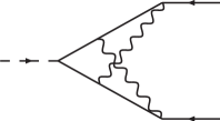
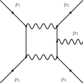
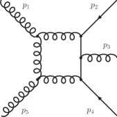
Figure 1: The master integrals V6l4m1 and F5l2m and F5l3m.

At several occasions, we used the package sector_decomposition [10] (built on the C++ library GINAC [13]) for cross checks and felt a lack of simple treatment of Feynman integrals with numerators. For that reason, the interface CSectors was written; it will be made publicly available soon. The syntax is similar to that of AMBRE. The program input for the evaluation of the integral V6l4m1 is simple; we again choose $m=1,s=-11$, and the topology may be read from the arguments of propagator functions PR:

<< CSectors.m

Options[DoSectors]
SetOptions[DoSectors, TempFileDelete -> False, SetStrategy -> C]

n1 = n2 = n3 = n4 = n5 = n6 = n7 = 1;
m = 1; s = -11;
invariants = {p1^2 -> m^2, p2^2 -> m^2, p1 p2 -> (s - 2 m^2)/2};

DoSectors[{1},
  {PR[k1,0,n1]       PR[k2,0,n2]       PR[k1+p1,m,n3]
   PR[k1+k2+p1,m,n5] PR[k1+k2-p2,m,n6] PR[k2-p2,m,n7]},
   {k2, k1}, invariants][-4, 2]

Here, the numerator is 1 (see the first argument $\{1\}$ of DoSectors), and the output contains the functions $U_{2}$ and $F_{2}$:

Using strategy C
U = x3 x4+x3 x5+x4 x5+x3 x6+x5 x6+x2 (x3+x4+x6)+x1 (x2+x4+x5+x6)

F = x1 x4^2+13 x1 x4 x5+x4^2 x5+x1 x5^2+x4 x5^2+13 x1 x4 x6
+2 x1 x5 x6+13 x4 x5 x6+x5^2 x6+x1 x6^2+x5 x6^2+x3^2 (x4+x5+x6)
+x2(x3^2+x4^2+13 x4 x6+x6^2+x3 (2 x4+13 x6))+x3 (x4^2+(x5+x6)^2
+x4 (2x5+13 x6))

Notice the presence of a $U$-function and the complexity of the $F$-function (compared to $U=1$ and f1 and f2 in the loop-by-loop MB-approach) due to the non-sequential, direct performance of both momentum integrals at once. Both $U$ and $F$ are evidently positive semi-definite. The numerical result for the Feynman integral is:

$$\mathtt{V6l4m1}(-s)^{2\varepsilon}=-0.052210~{}\frac{1}{\varepsilon}-0.17004+0.24634~{}\varepsilon+4.8773~{}\varepsilon^{2}+{\mathcal{O}}(\varepsilon^{3}).$$ (20)

The numbers may be compared to (11). We obtained a third numerical result, also by sector decomposition, with the Mathematica package FIESTA [14]:

$$\mathtt{V6l4m1}(-s)^{2\varepsilon}=-0.052208~{}\frac{1}{\varepsilon}-0.17002+0.24622~{}\varepsilon+4.8746~{}\varepsilon^{2}+{\mathcal{O}}(\varepsilon^{3}).$$ (21)

The most accurate result can be obtained with an analytical representation based on harmonic polylogarithmic functions [15, 16] obtained by solving a system of differential equations [17]:

$$\mathtt{V6l4m1}(-s)^{2\varepsilon}=-0.0522082~{}\frac{1}{\varepsilon}-0.170013+0.246253~{}\varepsilon+4.87500~{}\varepsilon^{2}+{\mathcal{O}}(\varepsilon^{3}).$$ (22)

All displayed digits are accurate here.

4 hexagon.m

The Mathematica package hexagon v. 1.0 (19 Sep 2008) was released quite recently [30 Sep 2008] at http://www-zeuthen.desy.de/theory/research/CAS.html. It may be used for the reduction of one-loop tensor 5- and 6-point Feynman integrals up to ranks $R=4$ and $R=3$, respectively, to scalar 3- and 4-point Feynman integrals. The latter have to be evaluated by some other package like LoopTools [18, 19] (case of only massive internal lines) or QCDloops [20] (general case); both these packages make also use of FF [21]. The formalism underlying this reduction and a short decsription as well as numerical examples may be found elsewhere [22, 23, 24, 25] so that we may hold this write-up short here. We only mention that it does not use Feynman parameters, but is based on recurrence relations with dimensional shifts [26]. In this approach, we have shown quite recently how to cancel explicitely and completely the inverse powers of the leading Gram determinant. hexagon was the first publicly available tensor reduction program for 5- and 6-point Feynman integrals with arbitrary internal masses. Now, also GOLEM95 [27] became public, but in the released version it handles so far only massless internal particles.

5 Summary

We described new features of the packages AMBRE and hexagon and of the interface
CSectors.

- [1] G. Balossini, C. Bignamini, C. M. Carloni Calame, G. Montagna, O. Nicrosini and F. Piccinini, Mini-review on Monte Carlo programs for Bhabha scattering, Nucl. Phys. Proc. Suppl. 183 (2008) 168, [arXiv:0806.4909 [hep-ph]].
- [2] A. Denner and S. Pozzorini, An algorithm for the high-energy expansion of multi-loop diagrams to next-to-leading logarithmic accuracy, Nucl. Phys. B717 (2005) 48–85, [hep-ph/0408068].
- [3] M. Czakon, J. Gluza, and T. Riemann, Master integrals for massive two-loop Bhabha scattering in QED, Phys. Rev. D71 (2005) 073009, [hep-ph/0412164].
- [4] J. Gluza, K. Kajda, and T. Riemann, AMBRE - a Mathematica package for the construction of Mellin-Barnes representations for Feynman integrals, Comput. Phys. Commun. 177 (2007) 879–893, [arXiv:0704.2423 [hep-ph]].
- [5] M. Czakon, A. Mitov, and S. Moch, Heavy-quark production in gluon fusion at two loops in QCD, Nucl. Phys. B798 (2008) 210–250, [0707.4139].
- [6] M. Czakon, Automatized analytic continuation of Mellin-Barnes integrals, Comput. Phys. Commun. 175 (2006) 559–571, [hep-ph/0511200].
- [7] J. Gluza, F. Haas, K. Kajda, and T. Riemann, Automatizing the application of Mellin-Barnes representations for Feynman integrals, PoS (ACAT) (2007) 081, [arXiv:0707.3567 [hep-ph]].
- [8] J. Gluza and T. Riemann, New results for 5-point functions, Proc. LCWS, Hamburg (2007) [arXiv:0712.2969 [hep-ph]]. See also at http://www-zeuthen.desy.de/riemanns/LCWS07-Loops.htm.
- [9] T. Binoth and G. Heinrich, An automatized algorithm to compute infrared divergent multi-loop integrals, Nucl. Phys. B585 (2000) 741–759, [http://arXiv.org/abs/hep-ph/0004013v.2].
- [10] C. Bogner and S. Weinzierl, Resolution of singularities for multi-loop integrals, Comput. Phys. Commun. 178 (2008) 596–610, [0709.4092].
- [11] G. Heinrich, Sector Decomposition, Int. J. Mod. Phys. A23 (2008) 1457–1486, [0803.4177].
- [12] A. V. Smirnov and V. A. Smirnov, Hepp and Speer Sectors within Modern Strategies of Sector Decomposition, 0812.4700.
- [13] C. Bauer, A. Frink, and R. Kreckel, Introduction to the GiNaC framework for symbolic computation within the C++ programming language, J. Symbolic Computation 33 (2002) 1, [cs.sc/0004015].
- [14] A. V. Smirnov and M. N. Tentyukov, Feynman Integral Evaluation by a Sector decomposiTion Approach (FIESTA), 0807.4129.
- [15] E. Remiddi and J. Vermaseren, Harmonic polylogarithms, Int. J. Mod. Phys. A15 (2000) 725–754, [hep-ph/9905237].
- [16] D. Maitre, HPL, a Mathematica implementation of the harmonic polylogarithms, Comput. Phys. Commun. 174 (2006) 222–240, [hep-ph/0507152].
- [17] J. Gluza and T. Riemann, unpublished.
- [18] T. Hahn and M. Rauch, News from formcalc and looptools, Nucl. Phys. Proc. Suppl. 157 (2006) 236–240, [hep-ph/0601248].
- [19] T. Hahn and M. Perez-Victoria, Automatized one-loop calculations in four and d dimensions, Comput. Phys. Commun. 118 (1999) 153, [http://arXiv.org/abs/hep-ph/9807565].
- [20] R. K. Ellis and G. Zanderighi, Scalar one-loop integrals for QCD, JHEP 02 (2008) 002, [0712.1851].
- [21] G. van Oldenborgh, Ff: A package to evaluate one loop Feynman diagrams, Comput. Phys. Commun. 66 (1991) 1.
- [22] J. Fleischer, J. Gluza, K. Kajda, and T. Riemann, Pentagon diagrams of Bhabha scattering, Acta Phys. Polon. B38 (2007) 3529–3536, [0710.5100].
- [23] T. Diakonidis, J. Fleischer, J. Gluza, K. Kajda, T. Riemann, and J. B. Tausk, On the tensor reduction of one-loop pentagons and hexagons, Nucl. Phys. Proc. Suppl. 183 (2008) 109–115, [0807.2984].
- [24] T. Diakonidis, J. Fleischer, J. Gluza, K. Kajda, T. Riemann, and J. B. Tausk, A complete reduction of one-loop tensor 5- and 6-point integrals, 0812.2134.
- [25] T. Diakonidis, “Reduction Method for One-loop Tensor 5- and 6-point Integrals Revisited.” To appear in Proc. of LCWS08 and ILC08, arXiv:0901.4455.
- [26] J. Fleischer, F. Jegerlehner, and O. Tarasov, Algebraic reduction of one-loop Feynman graph amplitudes, Nucl. Phys. B566 (2000) 423–440, [http://arXiv.org/abs/hep-ph/9907327].
- [27] T. Binoth, J. P. Guillet, G. Heinrich, E. Pilon, and T. Reiter, Golem95: a numerical program to calculate one-loop tensor integrals with up to six external legs, arXiv:0810.0992.