Optimal broadening of finite energy spectra in the numerical renormalization group: application to dissipative dynamics in two-level systems

Abstract

Numerical renormalization group (NRG) calculations of quantum impurity models, based on a logarithmic discretization in energy of electronic or bosonic Hamiltonians, provide a powerful tool to describe physics involving widely separated energy scales, as typically encountered in nanostructures and strongly correlated materials. This main advantage of the NRG was however considered a drawback for resolving sharp spectral features at finite energy, such as dissipative atomic peaks. Surprisingly, we find a bunching of many-body levels in NRG spectra near dissipative resonances, and exploit this by combining the widely-used Oliveira’s $z$-trick, using an averaging over few discrete NRG spectra, with an optimized frequency-dependent broadening parameter $b(\omega)$. This strategy offers a tremendous gain in computational power and extracts all the needed information from the raw NRG data without a priori knowledge of the various energy scales at play. As an application we investigate with high precision the crossover from coherent to incoherent dynamics in the spin boson model.

A general hallmark of many-particle interaction, as found in a variety of condensed matter systems such as nanostructures and strongly correlated materials, lies in the presence of several energy scales, possibly widely separated from each other due to renormalization and dynamical effects. Two well-studied examples found in electronic systems concern the Kondo effect for magnetic impurities in metals and Fermi liquids in proximity to a Mott insulating phase, two instances where low-energy quasiparticles emerge below a typical temperature which is quite reduced from the bare Fermi energy Hewson . These low-lying excitations do however coexist with higher energy atomic levels, also broadened and displaced in a strong manner from their bare atomistic values due to the dissipation brought by the electronic environment. Such complex physical effects, taking place on a broad range of energies, entail great practical difficulties for most direct numerical approaches. These are partially lifted using Wilson’s original idea of the logarithmic discretization Wilson ; Krishnamurthy , as implemented in numerical renormalization group calculations (see Ref. Bulla1, for a recent review). This technique has been improved in the last twenty years to calculate static and dynamic quantities both for fermionic Costi1 and bosonic quantum impurity models Tong . Important practical applications until now involve the calculation of transport in the Kondo regime for Kondo alloys and artificial quantum dots Costi2 , as well as the accurate description of the zero-temperature Mott transition by combining NRG Bulla2 with Dynamical Mean Field Theory (DMFT) DMFT . More generally, exponentially small energy scales are also found in the vicinity of quantum critical points Sachdev , so that impurity models provide a simplified testbed for the theory of quantum critical phenomena Vojta . Again the NRG is the ideal technique for studying such impurity quantum phase transitions Bulla1 , with potential implications for artificial nanostructures Potok ; Roch .

Despite these successes, the foundation of NRG on a logarithmic discretization mesh implies a loss in accuracy for the high energy spectral features, which has plagued most calculations so far. Not only are atomic-like excitations physically observable, using photoemission or tunneling spectroscopies, but they may also be intimately tied to the low-energy excitations. Such interesting behavior occurs in the vicinity of the Mott metal-insulator transition DMFT , where the self-consistently determined electronic environment in the DMFT picture shows electronic states violently redistributed over all energy scales. The numerical cost of converging the DMFT equations certainly requires efficient and accurate NRG calculations for the spectral functions, without a priori knowledge of the excitations involved. For this reason, the idea of averaging over $N_{z}$ realization of the Wilson chain, using the so-called $z$-trick Oliveira1 to fill in the missing spectral information (to be discussed later on), seems prohibitive for most practical calculations, and offers a limited gain for very narrow spectral structures (see Ref. Zitko, for a detailed study).

In this Rapid Communication, we show that the broadening procedure used to smoothen the discrete NRG data is one critical step for obtaining an optimal resolution at all energies. We henceforth develop a simple adaptive procedure where the standard broadening parameter $b$ is taken to be frequency dependent. This choice is dictated by our surprising observation that the density of many-body NRG levels increases sharply as soon as narrow atomic resonances are encountered. Together with the usual $z$-trick, combining several but reasonably few NRG calculations, this extra $b(\omega)$-trick allows to compute finite frequency spectra using as little as $N_{z}=10$ NRG calculations, in situations where large scale NRG $z$-averaging would be prohibitive. An improved broadening procedure leading to errors in spectral functions limited to few percents could constitute a further step in applying the NRG to a wider class of problems, such as DMFT+NRG calculations.

In order to explicitly demonstrate these ideas, we focus on the simplest quantum impurity model, namely the spin boson Hamiltonian:

$$H=\frac{\Delta}{2}\,\sigma^{x}+\frac{\lambda}{2}\,\sigma^{z}\sum_{i}(a^{\dagger}_{i}+a^{\phantom{\dagger}}_{i})+\sum_{i}\omega_{i}a^{\dagger}_{i}a^{\phantom{\dagger}}_{i}\,,$$ (1)

that involves a two-level system, described by a quantum spin $1/2$, and a bosonic bath $a^{\dagger}_{i}$ with continuous spectrum $\omega_{i}$ of energies. $\Delta$ is a transverse magnetic field, while the coupling constant $\lambda$ controls the strength of longitudinal dissipation. The bosonic spectrum is assumed to be sub-ohmic with bath exponent $0<s\leq 1$ (this includes the well-studied ohmic case $s=1$):

$$J(\omega)\equiv\sum_{i}\pi\lambda^{2}\delta(\omega-\omega_{i})=2\pi\alpha\omega_{c}^{1-s}\omega^{s}\theta(\omega)\theta(\omega_{c}-\omega)$$ (2)

where $\omega_{c}$ is a high-energy cutoff. For small values of the dissipation $\alpha$, this model is known to exhibit coherent precession of the spin around the $x$ axis at zero temperature. By increasing the coupling to the bath for values of $s\lesssim 1$, Rabi oscillations are progressively damped Leggett , before the two-level system localizes in one potential minima via a quantum phase transition Tong . When $s\gtrsim 0$ however, the phenomena of localization and decoherence occur in reverse order Anders . Despite its simplicity, this model embodies all the effects typical of strong correlations: low-energy scales are indeed dynamically generated near the localization transition, while discrete spin excitations due to the transverse field $\Delta$ are deeply affected by the bosonic environment, that leads to broadening and frequency shift in the magnetic response

$$C(\omega)=\frac{1}{2\pi}\int_{-\infty}^{+\infty}\!\!\!\!{\rm d}t\,C(t)e^{i\omega t}$$ (3)

with $C(t)=\frac{1}{2}\langle[\sigma_{z}(t),\sigma_{z}]\rangle$ the spin autocorrelation function.

The implementation of the NRG procedure follows the standard route Wilson as discussed in Ref. Tong, for the extension to bosonic Hamiltonians. The bosonic band (2) is logarithmically discretized with the Wilson parameter $\Lambda>1$, first on the highest energy interval $[\Lambda^{-z}\omega_{c},\omega_{c}]$, and then iteratively on successive decreasing energy windows $[\Lambda^{-n-z}\omega_{c},\Lambda^{-n-z+1}\omega_{c}]$ for $n$ strictly positive integer. This also introduces the crucial $z$ parameter ($0<z<1$) that is used to average over $N_{z}$ Wilson chains Oliveira1 , allowing to obtain better resolution on the finite energy states. The rest of the NRG follows Ref. Tong, , coupling iteratively the kept energy levels up to iteration $n$ to the states living in the shell $n+1$, and truncating the successive Hamiltonians to keep up with a manageable number of eigenstates. All subsequent calculations were performed with $\Lambda=2$, $N_{b}=8$ kept bosonic states on the added bosonic “site”, and $N=160$ kept NRG states, ensuring good convergence. The resulting discrete spectra at successive NRG iterations are combined using the interpolation scheme proposed in Ref. Bulla3, (see however Ref. Weichselbaum, for a more rigorous implementation), leading to a set of $z$-dependent many-body energy levels $\epsilon_{a,z}$ labelled by quantum number $a$. The spin-spin correlation function is thus readily obtained at zero temperature as:

$$C(\omega)=\frac{1}{2N_{z}}\sum_{a,z}|\langle 0,z|\sigma_{z}|a,z\rangle|^{2}\delta\left(|\omega|+\epsilon_{0,z}-\epsilon_{a,z}\right)$$ (4)

where $\epsilon_{0,z}$ is the ground state energy, and these raw NRG data are displayed on Fig. 1, to be discussed below.

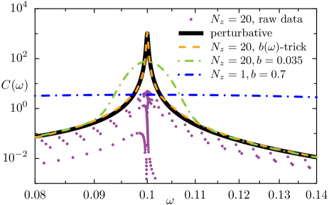
Figure 1: (Color online) Spin susceptibility $C(\omega)$ of the sub-ohmic spin boson model at $s=0.1$, $\Delta=0.1\omega_{c}$ and $\alpha=0.000125$. Raw data $|\langle 0,z|\sigma_{z}|a,z\rangle|^{2}/[2N_{z}(\epsilon_{a,z}-\epsilon_{0,z})]$ are given as circles for $N_{z}=20$ combined NRG calculations, solid line is the perturbative result (6), and the three dashed lines are the various NRG broadenings discussed in the text.

Let us now discuss the general structure of the NRG spectra. For a single NRG calculation with a given value of $z$, the a priori energy resolution at the scale $\omega_{N}=\Lambda^{-N-z}$ is $\delta\omega_{N}=\Lambda^{-N-z}-\Lambda^{-N-z-1}=(1-\Lambda^{-1})\omega_{N}$, so that the resolution degrades at increasing energy. For obtaining smooth NRG spectra, the delta-peaks in (4) are usually broadened Bulla1 at energy $\omega_{N}$ on the same scale:

$$\delta\left(|\omega|-\omega_{N}\right)\rightarrow\frac{e^{-b^{2}/4}}{\omega_{N}b\sqrt{\pi}}e^{-[\log(|\omega|/\omega_{N})^{2}/b]^{2}}$$ (5)

with $b\approx 0.7$ typically. Combining $N_{z}$ NRG runs using the $z$-averaging in (1) allows in principle to improve by a factor $N_{z}$ the accuracy at high energy, since the broadening parameter may now be decreased down to $b=0.7/N_{z}$. This procedure actually faces two problems: i) for very sharp resonances (typically several orders of magnitude narrower that the natural high-energy cutoff), parallelizing $N_{z}\gg 10$ NRG calculations becomes too prohibitive, especially with the aim of DMFT simulations; ii) states far from the resonances can then be too much underbroadened, so that oscillations of period $\Lambda/N_{z}$ can become quite prominent. In this view, quantitative spectra can be accurately extracted from the NRG data only in the continuum limit, either with $\Lambda\rightarrow 1$ or $N_{z}\rightarrow+\infty$, as assumed in the previous literature Zitko ; Oliveira2 ; Weichselbaum2 .

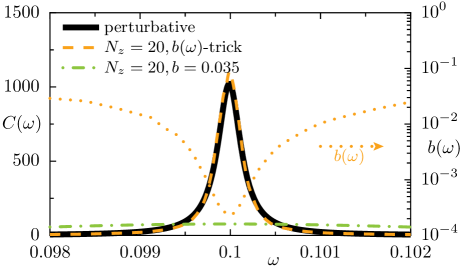
Figure 2: (Color online) Comparison of various broadening procedures near the resonance for the parameters of Fig. 1: standard interleaved averaging with $N_{z}=20$ and $b=0.7/N_{z}=0.035$ (dash-dotted line), $b(\omega)$-trick with $b_{0}=0.12$ (dashed line), and analytical result (full line). The adaptive broadening parameter $b(\omega)$ is also given (note the logarithmic scale on the right).

We wish to show however that NRG provides much more information close to dissipative resonances than usually expected. For this purpose, we closely examine the raw NRG spectra for resonance widths as small as $10^{-4}\omega_{c}$, using reasonably few interleaved averaging $N_{z}=20$, much smaller that the naively needed $10^{4}$ NRG runs. Fig. 1 shows that for frequencies far from the resonance located at $\Delta$, the highest weight NRG states come in packets of $N_{z}$ peaks for a given Wilson shell. Surprisingly, the density of NRG eigenstates demonstrates a huge increase precisely at the peak value, so that information about the resonance width and height seems really encoded in the discrete results! The standard broadening $b=0.7/N_{z}=0.035$ is however way too large to benefit from this effect, and the corresponding smoothed spectra are indeed completely inaccurate. For definite comparison, we have plotted the analytical result obtained from the expansion at weak dissipation Shnirman :

$$C(\omega) = -\frac{1}{\pi}{{\mathrm{Im}}}\frac{\omega-\Sigma(\omega)}{\omega[\omega-\Sigma(\omega)]-\Delta^{2}}$$ (6)

$$\Sigma(\omega) = \int\frac{{{\mathrm{d}}}\epsilon}{\pi}\frac{J(\epsilon)}{\omega-\epsilon+i0^{+}}=\int_{0}^{\omega_{c}}\!\!{{\mathrm{d}}}\epsilon\,\frac{2\alpha\omega_{c}^{1-s}\epsilon^{s}}{\omega-\epsilon+i0^{+}}.$$

In order to judiciously exploit this unexpected finding, the straightforward idea we follow here is to adapt the broadening parameter $b$ in (5) to the frequency dependence of the local density of NRG peaks. A very natural approach adapted to the NRG logarithmic discretization is to extract $b(\omega)$ from the logarithmic derivative of the integrated spectrum up to frequency $\omega$:

$$b(\omega)=\frac{b_{0}}{2}\left(\left[q+\frac{{{\mathrm{d}}}\log\int_{0}^{\omega}C}{{{\mathrm{d}}}\log\omega}\right]^{-1}\!\!\!\!\!\!+\!\left[q+\frac{{{\mathrm{d}}}\log\int_{+\infty}^{\omega}C}{{{\mathrm{d}}}\log\omega}\right]^{-1}\right)$$ (7)

where $q\simeq 1$ is regularization parameter, whose precise value is not sensitive to the final results, and $b_{0}$ sets the typical broadening at very low and very high frequencies (far from the atomic resonances). Note indeed that we average in this expression two frequency sweeps from $\omega=0$ and $\omega=+\infty$ respectively, in order to treat on an equal basis low and high frequency tails. Because the actual NRG data is fully discrete (4), we extract $b(\omega)$ recursively using equation (7) on the broadened NRG spectra. This procedure converges after few iterations to the results displayed on Figs. 1 and 2.

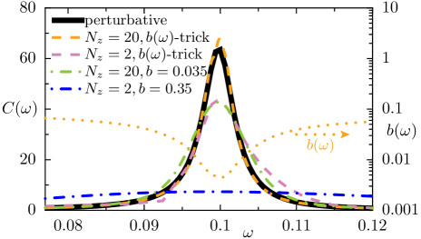
Figure 3: (Color online) Similar comparison as done on Fig. 2, with stronger dissipation $\alpha=0.02$. Optimized broadenings with $b(\omega)$-trick were done with $N_{z}=2,20$ and $b_{0}=0.6,0.12$ respectively.

Given the small numerical effort devoted to generate these NRG data, the quality of final result is quite astonishing. The reason for this success is given on Fig. 2, where the $b(\omega)$ parameter takes values as small as $10^{-4}$ at the resonance, while it increases drastically far away from it, naturally cancelling out a great part of the NRG oscillations due to the discretization of the Wilson chain. We emphasize that the only free parameter is the typical low-frequency broadening $b_{0}$ in (7), which is easily adjusted: we always find a range of $b_{0}$ values where the self-consistently broadened spectrum is relatively independent of the chosen $b_{0}$. More generally, one can also avoid the use of Ansatz (7) by determining $b(\omega)$ from estimates of the local density of highest weight states in the raw NRG data, giving similar results. Large scale NRG simulations with $N_{z}\gg 10$ and fixed $b$, as performed e.g. in Zitko , may thus benefit greatly from an adaptive broadening procedure. We also note that the high frequency tails are also faithfully reproduced using the $b(\omega)$-trick. Finally, in situations where relatively broader resonances are present, we show that quantitative results can be obtained at lower computational cost, by decreasing significantly the number of $z$-averaging even as low as $N_{z}<5$, see Fig. 3.

In order to check that our broadening procedure is completely robust for the whole range of parameters in the model (1), we investigate the effect of increasing dissipation for several bath exponent values $s$. The quantitative comparison of the Rabi resonance to the analytical formula (6) in its domain of validity, namely $\alpha\ll 1$, gives us indeed confidence in the adaptative method. This is proved on Fig. 4 and 5, which consider the same parameters as in Ref. Anders, , with important quantitative improvement.

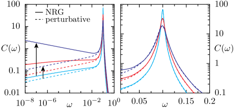
Figure 4: (Color online) Comparison of optimized NRG spectra (solid lines) and perturbative calculations (dashed lines) with bath exponent $s=0.1$, $\Delta=0.1\omega_{c}$ and increasing values (arrow) of dissipation $\alpha=0.002,0.004,0.007$.

For the small value of $s=0.1$ taken on Fig. 4, the perfect matching of the NRG data on the resonance to the lowest order calculation in $\alpha$ shows that the dissipation mechanism does not care for the low-energy behavior of the spin dynamics, even at the quantum critical point Tong ; Anders where the spin localizes for the values $\alpha_{c}=0.0071$ and $0.105$ with $s=0.1$ and $0.5$ respectively ($\Delta/\omega_{c}=0.1$ and $\Lambda=2$ here). Interestingly, the low-energy tails show significant deviations from the analytical result (6) even far from the quantum phase transition, so that lowest-order calculations Shnirman do not apply for the long-time dynamics. Improved resummation of the perturbation theory to all orders in $\alpha$ will be considered in a forthcoming work Florens . For the intermediate value $s=0.5$ shown on Fig. 5, clear non-perturbative effects on the resonance are seen inbetween the weak coupling regime and the quantum critical point, so that perturbation theory in $\alpha$ breaks down.

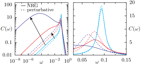
Figure 5: (Color online) Similar plot as on Fig. 4, with bath exponent $s=0.5$, $\Delta=0.1\omega_{c}$ and $\alpha=0.02,0.06,0.10$.

To conclude, we have investigated the properties of discrete NRG spectra near atomic states in the spin boson model, and found that a bunching of the many-body levels occurs whenever sharp resonances are encountered. An adaptive broadening scheme was proposed, showing a drastic improvement in computation power for the calculation of accurate spectral functions over the whole energy range. This procedure will certainly allow to take further advantage of the potentialities of the NRG in a wide range of physical situations, from ab-initio calculations for magnetic impurities in metals Costi3 to the difficult problem of simulating strongly correlated materials in the framework of the Dynamical Mean Field Theory DMFT .

References

- (1) A. C. Hewson, The Kondo Problem to Heavy Fermions, Cambridge University Press, Cambridge (1996).
- (2) K. G. Wilson, Rev. Mod. Phys. 47, 773 (1975).
- (3) H. R. Krishna-murthy, J. W. Wilkins and K. G. Wilson, Phys. Rev. B 21 1003 (1980).
- (4) R. Bulla, T. Costi and T. Pruschke, Rev. Mod. Phys. 80, 395 (2008).
- (5) T. A. Costi, A. C. Hewson and V. Zlatic, J. Phys.: Condens. Matter 6, 2519 (1994).
- (6) R. Bulla, H. J. Lee, N. H. Tong and M. Vojta, Phys. Rev. B 71, 045122 (2005).
- (7) T. A. Costi, Phys. Rev. Lett. 85, 1504 (2000).
- (8) R. Bulla, Phys. Rev. Lett. 83, 136 (1999).
- (9) A. Georges, G. Kotliar, W. Krauth and M. Rozenberg, Rev. Mod. Phys. 68, 13 (1996).
- (10) S. Sachdev, Quantum Phase Transitions, Cambridge University Press, Cambridge (1999).
- (11) M. Vojta, Phil. Mag. 86, 1807 (2006).
- (12) R. M. Potok, I. G. Rau, H. Shtrikman, Y. Oreg, and D. Goldhaber-Gordon, Nature 446, 167 (2007).
- (13) N. Roch, S. Florens, V. Bouchiat, W. Wernsdorfer and F. Balestro, Nature 453, 633 (2008).
- (14) W. C. Oliveira and L. N. Oliveira, Phys. Rev. B 49, 11986 (1994).
- (15) R. Zitko and T. Pruschke, Phys. Rev. B 79, 085106 (2009).
- (16) A. J. Leggett, S. Chakravarty, A. T. Dorsey, M. P. A. Fisher, A. Garg and W. Zwerger, Rev. Mod. Phys. 59, 1 (1987).
- (17) F. B. Anders, R. Bulla and M. Vojta, Phys. Rev. Lett. 98, 210402 (2007).
- (18) R. Bulla, T. A. Costi, and D. Vollhardt, Phys. Rev. B64, 045103 (2001).
- (19) A. Weichselbaum and J. von Delft, Phys. Rev. Lett. 99, 076402 (2007); R. Peters, T. Pruschke and F. B. Anders, Phys. Rev. B 74, 245114 (2006).
- (20) V. L. Campo and L. N. Oliveira, Phys. Rev. B 72, 104432 (2005).
- (21) A. Weichselbaum, F. Verstraete, U. Schollwöck, J. I. Cirac and J. von Delft, preprint arXiv:cond-mat/0504305.
- (22) A. Shnirman and Y. Makhlin, Phys. Rev. Lett. 91, 207204 (2003).
- (23) S. Florens, A. Freyn, R. Narayanan and D. Venturelli, in preparation.
- (24) T. A. Costi et al., Phys. Rev. Lett. 102, 056802 (2009).