Monte Carlo Determination of the Low-Energy Constants of a Spin 1/2 Heisenberg Model with Spatial Anisotropy

Abstract

Motivated by the possible mechanism for the pinning of the electronic liquid crystal direction in YBCO as proposed in Pardini08 , we use the first principles Monte Carlo method to study the spin 1/2 Heisenberg model with antiferromagnetic couplings $J_{1}$ and $J_{2}$ on the square lattice. In particular, the low-energy constants spin stiffness $\rho_{s}$, staggered magnitization ${\cal M}_{s}$ and spin wave velocity $c$ are determined by fitting the Monte Carlo data to the predictions of magnon chiral perturbation theory. Further, the spin stiffnesses $\rho_{s1}$ and $\rho_{s2}$ as a function of the ratio $J_{2}/J_{1}$ of the couplings are investigated in detail. Although we find a good agreement between our results with those obtained by the series expansion method in the weakly anisotropic regime, for strong anisotropy we observe discrepancies.

Introduction.— Understanding the mechanism responsible for high-temperature superconductivity in cuprate materials remains one of the most active research fields in condensed matter physics. Unfortunately, the theoretical understanding of the high-$T_{c}$ materials using analytic methods as well as first principles Monte Carlo simulations is hindered by the strong electron correlations in these materials. Despite this difficulty, much effort has been devoted to investigating the properties of the relevant $t$-$J$-type models for the high-$T_{c}$ cuprates Eder96 ; Lee97 ; Hamer98 ; Brunner00 . Although a conclusive agreement regarding the mechanism responsible for the high-$T_{c}$ phenomena has not been reached yet, it is known that the high-$T_{c}$ cuprate superconductors are obtained by doping the antiferromagnetic insulators with charge carriers. This has triggered vigorous studies of undoped and lightly doped antiferromagnets. Today, the undoped antiferromagnets on the square lattice such as La₂CuO₄ are among the quantitatively best understood condensed matter systems.

Spatially anisotropic Heisenberg models have been studied intensely due to their phenomenological importance as well as from the perspective of theoretical interest Parola93 ; Sandvik99 ; Irkhin00 ; Kim00 . For example, numerical evidence indicates that the anisotropic Heisenberg model with staggered arrangement of the antiferromagnetic couplings may belong to a new universality class, in contradiction to the $O(3)$ universality predictions Wenzel08 . Further, it is argued that the Heisenberg model with spatially anisotropic couplings $J_{1}$ and $J_{2}$ is relevant to the newly discovered pinning effects of the electronic liquid crystal in the underdoped cuprate superconductor YBa₂Cu₃O_6.45 Hinkov2007 ; Hinkov2008 . It is observed that the YBa₂Cu₃O_6.45 compound has a tiny in-plane lattice anisotropy which is strong enough to pin the orientation of the electronic liquid crystal in a particular direction. The authors of Pardini08 demonstrated that the in-plane anisotropy of the spin stiffness of the Heisenberg model with spatially anisotropic couplings $J_{1}$ and $J_{2}$ can provide a possible mechanism for the pinning of the electronic liquid crystal direction in YBa₂Cu₃O_6.45.

Since the anisotropy of the spin stiffness in the spin 1/2 Heisenberg model with different antiferromagnetic couplings $J_{1}$ and $J_{2}$ has not been studied in detail before with first principles Monte Carlo methods, in this letter we perform a Monte Carlo calculation to determine the low-energy constants, namely the spin stiffnesses $\rho_{s1}$ and $\rho_{s2}$, staggered magnitization ${\cal M}_{s}$ and spin wave velocity $c$. In particular, we investigate the $J_{2}/J_{1}$-dependence of $\rho_{s1}$ and $\rho_{s2}$, and find good agreement with earlier studies Pardini08 using series expansion methods in the weakly anisotropic regime. Our this finding would lead to very strong pinning energy per Cu site in YBa₂Cu₃O_6.45 as claimed in Pardini08 . However, deviations appear as one moves toward strong anisotropy. We argue that the deviations observed between our results and the naive expectation might indicate an unexpected behavior of the spin-stiffness $\rho_{s}$ at extremely strong anisotropy.

Figure 1: The anisotropic Heisenberg model investigated in this study. $J_{1}$ and $J_{2}$ are the antiferromagnetic couplings in the $1$- and $2$-directions, respectively.

Microscopic Models and Corresponding Observables.— The Heisenberg model we consider in this study is defined by the Hamilton operator

$$H=\sum_{x}\Big{[}\,J_{1}\vec{S}_{x}\cdot\vec{S}_{x+\hat{1}}+J_{2}\vec{S}_{x}\cdot\vec{S}_{x+\hat{2}}\,\Big{]},$$ (1)

where $\hat{1}$ and $\hat{2}$ refer to the two spatial unit-vectors. Further, $J_{1}$ and $J_{2}$ in eq. (1) are the antiferromagnetic couplings in the $1$- and $2$-directions respectively. A physical quantity of central interest is the staggered susceptibility (corresponding to the third component of the staggered magnetization $M_{s}^{3}$) which is given by

$$\chi_{s} = \frac{1}{L_{1}L_{2}}\int_{0}^{\beta}dt\ \frac{1}{Z}\mbox{Tr}[M^{3}_{s}(0)M^{3}_{s}(t)\exp(-\beta H)].$$ (2)

Here $\beta$ is the inverse temperature, $L_{1}$ and $L_{2}$ are the spatial box sizes in the $1$- and $2$-direction, respectively, and $Z=\mbox{Tr}\exp(-\beta H)$ is the partition function. The staggered magnetization order parameter $\vec{M}_{s}$ is defined as $\vec{M}_{s}=\sum_{x}(-1)^{x_{1}+x_{2}}\vec{S}_{x}$. Another relevant quantity is the uniform susceptibility which is given by

$$\chi_{u} = \frac{1}{L_{1}L_{2}}\int_{0}^{\beta}dt\ \frac{1}{Z}\mbox{Tr}[M^{3}(0)M^{3}(t)\exp(-\beta H)].$$ (3)

Here $\vec{M}=\sum_{x}\vec{S}_{x}$ is the uniform magnetization. Both $\chi_{s}$ and $\chi_{u}$ can be measured very efficiently with the loop-cluster algorithm using improved estimators Wie94 . In particular, in the multi-cluster version of the algorithm the staggered susceptibility is given in terms of the cluster sizes $|{\cal C}|$ (which have the dimension of time), i.e. $\chi_{s}=\frac{1}{\beta L_{1}L_{2}}\left\langle\sum_{\cal C}|{\cal C}|^{2}\right\rangle$. Similarly, the uniform susceptibility $\chi_{u}=\frac{\beta}{L_{1}L_{2}}\left\langle W_{t}^{2}\right\rangle=\frac{\beta}{L_{1}L_{2}}\left\langle\sum_{\cal C}W_{t}({\cal C})^{2}\right\rangle$ is given in terms of the temporal winding number $W_{t}=\sum_{\cal C}W_{t}({\cal C})$ which is the sum of winding numbers $W_{t}({\cal C})$ of the loop-clusters ${\cal C}$ around the Euclidean time direction. Similarly, the spatial winding numbers are defined by $W_{i}=\sum_{\cal C}W_{i}({\cal C})$ with $i\in\{1,2\}$.

Low-Energy Effective Theory for Magnons.— Due to the spontaneous breaking of the $SU(2)_{s}$ spin symmetry down to its $U(1)_{s}$ subgroup, the low-energy physics of antiferromagnets is governed by two massless Goldstone bosons, the antiferromagnetic spin waves or magnons. The description of the low-energy magnon physics by an effective theory was pioneered by Chakravarty, Halperin, and Nelson in Cha89 . A systematic low-energy effective field theory for magnons was further developed in Neu89 ; Has90 ; Has91 . The staggered magnetization of an antiferromagnet is described by a unit-vector field $\vec{e}(x)$ in the coset space $SU(2)_{s}/U(1)_{s}=S^{2}$, i.e. $\vec{e}(x)=\big{(}e_{1}(x),e_{2}(x),e_{3}(x)\big{)}$ with $\vec{e}(x)^{2}=1$. Here $x=(x_{1},x_{2},t)$ denotes a point in (2+1)-dimensional space-time. To leading order, the Euclidean magnon low-energy effective action takes the form

$$S[\vec{e}\,] = \int^{L_{1}}_{0}dx_{1}\int^{L_{2}}_{0}dx_{2}\int^{\beta}_{0}\ dt\ \left(\frac{\rho_{s1}}{2}\partial_{1}\vec{e}\cdot\partial_{1}\vec{e}\right.$$ (4)

$$+\left.\frac{\rho_{s2}}{2}\partial_{2}\vec{e}\cdot\partial_{2}\vec{e}+\frac{\rho_{s}}{2c^{2}}\partial_{t}\vec{e}\cdot\partial_{t}\vec{e}\right),$$

where the index $i\in\{1,2\}$ labels the two spatial directions and $t$ refers to the Euclidean time-direction. The parameters $\rho_{s}=\sqrt{\rho_{s1}\rho_{s2}}$, $\rho_{s1}$ and $\rho_{s2}$ are the spin stiffness in the temporal and spatial directions, respectively, and $c$ is the spin wave velocity. Rescaling $x^{\prime}_{1}=(\rho_{s2}/\rho_{s1})^{1/4}x_{1}$ and $x^{\prime}_{2}=(\rho_{s1}/\rho_{s2})^{1/4}x_{2}$, eq. (4) can be rewritten as

$$S[\vec{e}\,] = \int^{L^{\prime}_{1}}_{0}dx^{\prime}_{1}\int^{L^{\prime}_{2}}_{0}dx^{\prime}_{2}\int^{\beta}_{0}dt\ \frac{\rho_{s}}{2}\Big{(}\partial^{\prime}_{i}\vec{e}\cdot\partial^{\prime}_{i}\vec{e}$$ (5)

$$+\frac{1}{c^{2}}\partial_{t}\vec{e}\cdot\partial_{t}\vec{e}\Big{)}.$$

Additionally requiring $L^{\prime}_{1}=L^{\prime}_{2}=L$ we obey the condition of square area. Notice the effective field theories described by eqs. (4) and (5) are valid as long as the conditions $L_{i}\beta\rho_{s1}\gg 1$ and $L_{i}\beta\rho_{s2}\gg 1$ for $i\in\{1,2\}$ hold, which is indeed the case for the set up of this study. Once these conditions are satisfied, the low-energy physics of the underlying microscopic model can be captured quantitatively by the effective field theory as demonstrated in Wie94 . Further, in the so-called cubical regime (to be defined later) which is relevant to our study, the cut-off effects appear in the free energy density only at next-to-next-to-next-to-leading order (NNNLO). The finite cut-off leads to higher-order terms in the effective Lagrangian due to the breaking of some symmetries and it introduces the cut-off dependence in the Fourier integrals (sums). By employing similar arguments as those presented in Has93 , one can show that higher-order corrections to eq. (4) contain four derivatives and the leading cut-off effect in the Fourier integrals (sums) enters the free energy density only at NNNLO. Therefore eq. (5) is sufficient to derive up to next-to-next-to-leading order (NNLO) contributions to the observables considered here. We have further verified that the inclusion of NNNLO contributions to the relevant observables considered here lead to statistically consistent results with those not taking such corrections into account. Hence the volume- and temperature- dependence of $\chi_{s}$ and $\chi_{u}$ up to NNLO (to be presented below) are sufficient to describe our numerical data quantitatively, and the finite cut-off effects are negligible. Using the above Euclidean action (5), detailed calculations of a variety of physical quantities including the NNLO contributions have been carried out in Has93 . Here we only quote the results that are relevant to our study, namely the finite-temperature and finite-volume effects of the staggered susceptibility and the uniform susceptibility. The aspect ratio of a spatially quadratic space-time box with box size $L$ is characterized by $l=(\beta c/L)^{1/3}\,,$ with which one distinguishes cubical space-time volumes with $\beta c\approx L$ from cylindrical ones with $\beta c\gg L$. In the cubical regime, the volume- and temperature-dependence of the staggered susceptibility is given by

$$\chi_{s} = \frac{{\cal M}_{s}^{2}L^{2}\beta}{3}\left\{1+2\frac{c}{\rho_{s}Ll}\beta_{1}(l)\right.$$ (6)

$$+\left.\left(\frac{c}{\rho_{s}Ll}\right)^{2}\left[\beta_{1}(l)^{2}+3\beta_{2}(l)\right]+O\left(\frac{1}{L^{3}}\right)\right\},$$

where ${\cal M}_{s}$ is the staggered magnetization density. Finally the uniform susceptibility takes the form

$$\chi_{u} = \frac{2\rho_{s}}{3c^{2}}\left\{1+\frac{1}{3}\frac{c}{\rho_{s}Ll}\widetilde{\beta}_{1}(l)+\frac{1}{3}\left(\frac{c}{\rho_{s}Ll}\right)^{2}\times\right.$$ (7)

$$\left.\left[\widetilde{\beta}_{2}(l)-\frac{1}{3}\widetilde{\beta}_{1}(l)^{2}-6\psi(l)\right]+O\left(\frac{1}{L^{3}}\right)\right\}.$$

In (6) and (7), the functions $\beta_{i}(l)$, $\widetilde{\beta}_{i}(l)$, and $\psi(l)$, which only depend on $l$, are shape coefficients of the space-time box defined in Has93 .

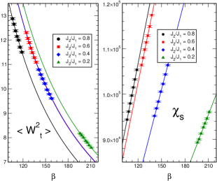
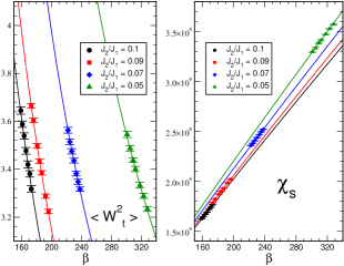
Figure 2: Comparison between our numerical results (data points) and the theoretical predictions (solid lines) which are obtained by using the low-energy parameters from the fits.

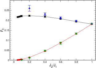
Figure 3: The $J_{2}/J_{1}$-dependence of the spin stiffness $\rho_{s1}$ and $\rho_{s2}$ of the anisotropic Heisenberg model. While the solid circles (black) and squares (red) are the Monte Carlo results of $\rho_{s1}$ and $\rho_{s2}$, respectively, the up and down triangles are the series expansion results of Pardini08 for $\rho_{s1}$ and $\rho_{s2}$, respectively. The solid lines are added to guide the eye.

Determination of the Low-Energy Parameters and Discussions.— In order to determine the low-energy constants for the anisotropic Heisenberg model given in (1), we have performed simulations within the range $0.05\leq J_{2}/J_{1}\leq 1.0$. The cubical regime is determined by the condition $\,\langle\sum_{C}W_{1}(C)^{2}\,\rangle\approx\langle\,\sum_{C}W_{2}(C)^{2}\,\rangle\approx\langle\,\sum_{C}W_{t}(C)^{2}\,\rangle$ (which implies $\beta c\approx L$). Notice that since $J_{2}\leq J_{1}$ in our simulations, one must increase the lattice size $L_{1}$ in order to fulfill the condition $\,\langle\sum_{C}W_{1}(C)^{2}\,\rangle=\langle\,\sum_{C}W_{2}(C)^{2}\,\rangle$ because eqs. (6) and (7) are obtained for a (2 + 1)-dimensional box with equal extent in the two spatial directions. Therefore, an interpolation of the data points is required in order to be able to use eqs. (6) and (7). Further, the low-energy parameters are extracted by fitting the Monte Carlo data to the effective field theory predictions. The quality of these fits is good as can be seen from figure 2 (the $\chi^{2}/{\text{d.o.f}}$ for all the fits is less than $1.25$). Figure 3 shows $\rho_{s1}$ and $\rho_{s2}$, obtained from the fits, as functions of the ratio of the antiferromagnetic couplings, $J_{2}/J_{1}$. The values of $\rho_{s1}$ ($\rho_{s2}$) obtained here agree quantitatively with those obtained using the series expansion in Pardini08 at $J_{2}/J_{1}=0.8$ and $0.6$ ($0.8$, $0.6$, $0.4$, and $0.2$). At $J_{2}/J_{1}=0.4$, the value we obtained for $\rho_{s1}$ is only slightly below the corresponding series expansion result in Pardini08 . However, sizable deviations begin to show up for stronger anisotropies. Further, we have not observed the saturation of $\rho_{s1}$ to a $1$-D limit, namely $0.25J_{1}$ as suggested in Pardini08 , even at $J_{2}/J_{1}$ as small as $0.05$. In particular, $\rho_{s1}$ decreases slightly as one moves from $J_{2}/J_{1}=0.1$ to $J_{2}/J_{1}=0.05$, although they still agree within statistical errors. Of course, one cannot rule out that the anisotropies in $J_{2}/J_{1}$ considered here are still too far away from the regime where this particular Heisenberg model can be effectively described by its $1$-D limit. On the other hand, the Heisenberg model considered here and its 1-D limit are two completely different systems, because spontaneous symmetry breaking appears only in 2-D, still $\xi=\infty$ in both cases. Further, the low-temperature behavior of $\chi_{u}$ in the 1-D system is known to be completely different from that of the 2-D system Egg94 ; Has93 . Although intuitively one might expect a continuous transition of $\rho_{s1}$, one cannot rule out an unexpected behavior of $\rho_{s1}$ as one moves from this Heisenberg model toward its 1-D limit. In particular, since earlier studies indicate that long-range order already sets in even for infinitesimal small $J_{2}/J_{1}$ Sandvik99 ; Affleck94 ; Miy95 , it would be interesting to consider even stronger anisotropies $J_{2}/J_{1}$ than those used in this study to see how $\rho_{s1}$ approaches its $1$-D limit. In addition to $\rho_{s1}$ and $\rho_{s2}$, we have obtained ${\cal M}_{s}$ and $c$ as functions of $J_{2}/J_{1}$ as well from the fits (figure 4). The values we obtained for ${\cal M}_{s}$ agree with earlier results in Sandvik99 , but have much smaller errors at strong anisotropies.

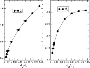
Figure 4: The $J_{2}/J_{1}$-dependence of the spin wave velocity $c$ (left) and the staggered magnitization density ${\cal M}_{s}$ (right) of the anisotropic Heisenberg model. The solid lines are added to guide the eye.

Next, we would like to turn to discussing the relevance of our results to the pinning effect observed empirically in YBa₂Cu₃O_6.45. In Pardini08 it is argued that the $J_{2}/J_{1}$ dependence of the spin-stiffnesses in the spatially anisotropic Heisenberg model studied in this work would lead to a very strong pinning energy per Cu site (one order of magnitude larger compared to the corresponding pinning energy in La₂CuO₄). To be more precise, it is the quantity $\kappa$ which is defined by $\rho_{s2}/\rho_{s1}=1+\kappa(J_{2}/J_{1}-1)$ in the weak anisotropy regime that results in the claim made in Pardini08 . Since the spin-stiffnesses calculated here agree with those obtained by series expansion in the weak anisotropy regime, which in turn implies that our $\kappa$ agrees with that in Pardini08 , we conclude that the pinning energy per Cu site is indeed very strong. Hence the in-plane anisotropy of the spin stiffness of the Heisenberg model with anisotropic couplings $J_{1}$ and $J_{2}$ can indeed provide a possible mechanism for the pinning of the electronic liquid crystal direction in YBa₂Cu₃O_6.45.

Conclusions.— In this note, we have numerically studied the Heisenberg model with anisotropic couplings $J_{1}$ and $J_{2}$ using a loop cluster algorithm. The coresponding low-energy constants are determined with high precision. Further, the $J_{2}/J_{1}$-dependence of $\rho_{s1}$ and $\rho_{s2}$ is investigated in detail and our results agree quantitatively with those obtained by series expansion Pardini08 in the weakly anisotropic regime. On the other hand, we observe discrepancies between our results and series expansion results in the strongly anisotropic regime. However, the results of our study still lead to very strong pinning energy per Cu site in YBa₂Cu₃O_6.45 which agrees with the claim made by the authors in Pardini08 . Finally we find that an unexpected behavior of $\rho_{s1}$ might be observed as one approaches much stronger anisotropy regime than those considered in this study.

We like to thank P. A. Lee, F. Niedermayer, B. C. Tiburzi, and U.-J. Wiese for useful discussions and comments on the manuscript. We also like to thank T. Pardini, R. R. P. Singh, and O. P. Sushkov for correspondence and providing their series expansion results in Pardini08 . The simulations in this study were performed using the ALPS library Troyer08 . This work is supported in part by funds provided by the Schweizerischer Nationalfonds (SNF).

References

- (1) T. Pardini, R. R. P. Singh, A. Katanin and O. P. Sushkov, Phys. Rev. B 78, 024439 (2008).
- (2) R. Eder, Y. Ohta, and G. A. Sawatzky, Phys. Rev. B55, R3414 (1996).
- (3) T. K. Lee and C. T. Shih, Phys. Rev. B55, R5983 (1997).
- (4) C. J. Hamer, W. Zheng, and J. Oitmaa, Phys. Rev. B58, 15508 (1998).
- (5) M. Brunner, F. F. Assaad, and A. Muramatsu, Phys. Rev. B62, 15480 (2000).
- (6) A. Parola, S. Storella, and Q. F. Zhong, Phys. Rev. Lett. 71, 4393 (1993).
- (7) A. W. Sandvik, Phys. Rev. Lett. 83, 3069 (1999).
- (8) V. Y. Irkhin and A. A. Katanin, Phys. Rev. B 61, 6757 (2000).
- (9) Y. J. Kim and R. Birgeneau, Phys. Rev. B 62, 6378 (2000).
- (10) S. Wenzel, L. Bogacz, and W. Janke, Phys. Rev. Lett 101, 127202 (2008).
- (11) V. Hinkov, P. Bourges, S. Pailhes, Y. Sidis, A. Ivanov, C. D. Frost, T. G. Perring, C. T. Lin, D. P. Chen, B. Keimer, Nature Physics 3, 780 (2007).
- (12) V. Hinkov et. al, Science 319, 597 (2008).
- (13) U.-J. Wiese and H.-P. Ying, Z. Phys. B 93, 147 (1994).
- (14) S. Chakravarty, B. I. Halperin, and D. R. Nelson, Phys. Rev. B 39, 2344 (1989).
- (15) H. Neuberger and T. Ziman, Phys. Rev. B 39, 2608 (1989).
- (16) P. Hasenfratz and H. Leutwyler, Nucl. Phys. B343, 241 (1990).
- (17) P. Hasenfratz and F. Niedermayer, Phys. Lett. B268, 231 (1991).
- (18) P. Hasenfratz and F. Niedermayer, Z. Phys. B 92, 91 (1993).
- (19) S. Eggert, I. Affleck, and M. Takahashi, Phys. Rev. Lett. 73, 332 (1994).
- (20) I. Affelck, M. P. Gelfand, and R. R. P. Singth, L. Phys. A 27, 7313 (1994).
- (21) T. Miyazaki, D. Yoshioka, and M. Ogata, Phys. Rev. B 51, 2966 (1995).
- (22) A. F. Albuquerque et. al, Journal of Magnetism and Magnetic Material 310, 1187 (2007).