Estimating black carbon aging time-scales with a particle-resolved aerosol model

Abstract

Understanding the aging process of aerosol particles is important for assessing their chemical reactivity, cloud condensation nuclei activity, radiative properties and health impacts. In this study we investigate the aging of black carbon containing particles in an idealized urban plume using a new approach, the particle-resolved aerosol model PartMC-MOSAIC. We present a method to estimate aging time-scales using an aging criterion based on cloud condensation nuclei activation. The results show a separation into a daytime regime where condensation dominates and a nighttime regime where coagulation dominates. For the chosen urban plume scenario, depending on the supersaturation threshold, the values for the aging time-scales vary between 0.06 hours and 10 hours during the day, and between 6 hours and 20 hours during the night.

, , ,

1 Introduction

Black carbon containing particles, or “soot” particles, are ubiquitous in the atmosphere and their role for regional and global climate has been widely recognized (IPCC, 2007). Since black carbon absorbs light (Horvath and Trier, 1993), it contributes to the aerosol radiative forcing, potentially partially offsetting the cooling effect of scattering aerosol particles such as sulfates (Menon et al., 2002).

Black carbon containing particles originate from the incomplete combustion of carbon containing material, hence emissions from traffic are an important contributor (Bond et al., 2004). Other important sources for black carbon include biomass burning and the combustion of coal by industrial processes. In this paper we focus on black carbon from traffic emissions. Measurements of vehicle emissions from gasoline and diesel cars show that the emitted particles are a complex mixture of many chemical species with the main constituents being black carbon and organic carbon (Medalia and Rivin, 1982; Toner et al., 2006). Trace concentrations of ionic and metallic species are also present (Kleeman et al., 2000). The exact composition depends on several factors, including the fuel type, the operating conditions and the condition of the individual vehicles.

During their transport in the atmosphere, the composition of these particle emissions are further modified. Coagulation, condensation and photochemistry are contributing processes, collectively known as aging (Weingartner et al., 1997). During this aging process the composition of the individual particles or, in other words, their mixing states change (Furutani et al., 2008). This impacts the particles’ physico-chemical properties including their chemical reactivity, radiative properties and health impacts. In particular, the aging process can change the particles’ hygroscopicity from initially hydrophobic to more hydrophylic, and hence change their ability to become cloud condensation nuclei (McFiggans et al., 2006; McMurry and Stolzenburg, 1989; Moffet et al., 2008; Cubison et al., 2008).

This is important as models and observations suggest that wet deposition represents 70–85% of the tropospheric sink for carbonaceous aerosol mass (Pöschl, 2005). As a consequence, to assess the budget and impact of black carbon, models need to capture the aging process adequately. Many global models have simulated both (fresh) hydrophobic black carbon and (aged) hydrophilic black carbon, which can be considered a minimal representation of the black carbon mixing state (Cooke et al., 1999; Lohmann et al., 1999; Koch, 2001; Croft et al., 2005). In such a framework only the hydrophilic black carbon is subject to in-cloud scavenging. The conversion from hydrophobic to hydrophilic is frequently modeled as a first-order system with the single parameter of aging rate or its inverse, the aging time-scale $\tau$ which represents the time-scale on which a population of black carbon containing particles transfers from the “fresh” category to the “aged” category.

While conceptually simple, the actual value of the aging time-scale $\tau$ is not well constrained. Koch (2001) and Croft et al. (2005) compared different aging parameterizations in global models and concluded that the model results critically depended on the respective formulation. Riemer et al. (2004) used mesoscale simulations to determine $\tau$. They derived the aging time-scale for black carbon particles as a function of height and time of the day, which suggested that assuming a single parameter for the black carbon aging time-scale is an oversimplification that will incorrectly estimate the black carbon burden. However, even though this treatment allowed more detailed insight into the aging process, it was still based on ad hoc aging rules inherent to the modal model framework that was used (Riemer et al., 2003).

Recently, Riemer et al. (2009) developed a particle-resolved aerosol model, PartMC-MOSAIC, which explicitly resolves the composition of individual particles in a given population of different types of aerosol particles, so that no ad hoc aging criteria needs to be invoked. They applied PartMC-MOSAIC in a Lagrangian box-model framework to an idealized urban plume scenario to study the evolution of urban aerosols due to coagulation and condensation over the course of 24 hours.

In this study, we build upon Riemer et al. (2009) and present a method for estimating aging time-scales of black carbon containing particles using PartMC-MOSAIC, based on the idealized urban plume scenario. We take the particle population simulated in Riemer et al. (2009) and use a CCN-based aging criteria to determine whether each individual particle is fresh or aged at every timestep, and how many particles transfer between the fresh and aged categories during each timestep. By fitting these results to a first-order bulk model of aerosol aging we are able to determine the aging timescale without making any a priori assumptions about the aging process. To our knowledge it is the first time that a method is presented for explicitly calculating aging time-scales.

Section 2 introduces the model system. In Section 3 we describe the idealized plume scenario that served as a basis for the time-scale estimation. Section 4 presents our method for deriving time-scales from our model and Section 5 shows the results. We summarize our findings in Section 6.

2 Model description

PartMC-MOSAIC is a particle-resolved model that simulates the evolution of individual aerosol particles and trace gases in a single parcel (or volume) of air moving along a specified trajectory. For each particle the mass of each constituent species is tracked, but the particle position in space is not simulated, making this a zero-dimensional or box model. In addition to coagulation and aerosol- and gas-phase chemistry, the model includes prescribed emissions of aerosols and gases, and mixing of the parcel with background air. The simulation results shown here use around 100,000 particles in a volume of around $16\rm\,cm^{3}$ (the precise values vary over the course of the simulation). We regard this volume as being representative of a much larger air parcel. The model accurately predicts both number and mass size distributions and is therefore suited for applications where either quantity is required. Details of PartMC-MOSAIC and the urban plume scenario are described in Riemer et al. (2009). Here we give a brief summary.

The simulation of the aerosol state proceeds by two mechanisms. First, the composition of each particle can change as species condense from the gas phase and evaporate to it. Second, the aerosol population can have particles added and removed, either by coagulation events between particles, by emissions, or by dilution. While condensation/evaporation is handled deterministically, emission, dilution and coagulation are treated with a stochastic approach.

Coagulation between aerosol particles is simulated in PartMC by generating a realization of a Poisson process with a Brownian coagulation kernel. For the large number of particles used here it is necessary to employ an efficient approximate simulation method. We developed a binned sampling method to efficiently sample from the highly multi-scale coagulation kernel (in our case the Brownian kernel) in the presence of a very non-uniform particle size distribution, which is described in detail in Riemer et al. (2009).

Particle emissions and dilution with background air are also implemented in a stochastic manner. Because we are using a finite number of particles to approximate the current aerosol population, we need to add a finite number of emitted particles to the volume at each timestep. Over time these finite particle samplings should approximate the continuum emission distribution, so the samplings at each timestep must be different. As for coagulation, we assume that emissions are memoryless, so that emission of each particle is uncorrelated with emission of any other particle. Under this assumption the appropriate statistics are Poisson distributed, whereby the distribution of finite particles is parametrized by the mean emission rate and distribution.

Lastly, we must also obtain a finite sampling of background particles that have diluted into our computational volume during each timestep. In addition, some of the particles in our current sample will dilute out of our volume and will be lost, so this must be sampled as well. Again, we assume that dilution is memoryless, so that dilution of each particle is uncorrelated with the dilution of any other particle or itself at other times, and that once a particle dilutes out it is lost.

We coupled the stochastic PartMC particle-resolved aerosol model to the deterministic MOSAIC gas- and aerosol-chemistry code (Zaveri et al., 2008) in a time- or operator-splitting fashion (Press et al., 2007, Section 20.3.3). MOSAIC treats all the globally important aerosol species including sulfate, nitrate, chloride, carbonate, ammonium, sodium, calcium, primary organic aerosol (POA), secondary organic aerosol (SOA), black carbon (BC), and inert inorganic mass.

MOSAIC consists of four computationally efficient modules: 1) the gas-phase photochemical mechanism CBM-Z (Zaveri and Peters, 1999); 2) the Multicomponent Taylor Expansion Method (MTEM) for estimating activity coefficients of electrolytes and ions in aqueous solutions (Zaveri et al., 2005b); 3) the Multicomponent Equilibrium Solver for Aerosols (MESA) for intra-particle solid-liquid partitioning (Zaveri et al., 2005a); and 4) the Adaptive Step Time-split Euler Method (ASTEM) for dynamic gas-particle partitioning over size- and composition-resolved aerosol (Zaveri et al., 2008). The version of MOSAIC implemented here also includes a treatment for SOA based on the SORGAM scheme (Schell et al., 2001).

3 Idealized urban plume scenario

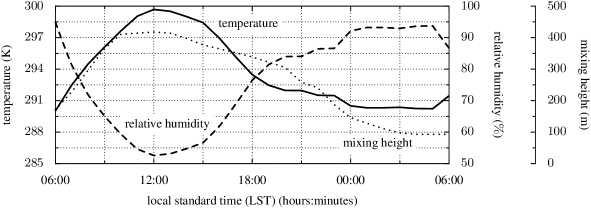
Figure 1: Time series of temperature, relative humidity, and mixing height over the course of the 24 hour simulation. The pressure and water mixing ratio were kept constant.

For our urban plume scenario, we tracked the evolution of gas phase species and aerosol particles in a Lagrangian air parcel that initially contained background air and was advected over and beyond a large urban area, as described in Riemer et al. (2009). The simulation started at 06:00 local standard time (LST), and during the advection process, primary trace gases and aerosol particles from different sources were emitted into the air parcel for the duration of 12 hours. After 18:00 LST, all emissions were switched off, and the evolution of the air parcel was tracked for another 12 hours. The time series of temperature, relative humidity and mixing height are shown in Figure 1.

Initial gas-phase and aerosol particle concentrations as well as gas phase and particle emissions were the same as in Riemer et al. (2009). The gas phase emissions varied throughout the emission time interval according to a typical diurnal cycle found in polluted urban areas.

The initial particle distribution, which was identical to the background aerosol distribution, was bimodal with Aitken and accumulation modes (Jaenicke, 1993). We assumed that it consisted of $\rm(NH_{4})_{2}SO_{4}$ and POA, as shown in Table 1. We considered three different types of carbonaceous aerosol emissions: 1) meat cooking aerosol, 2) diesel vehicle emissions, and 3) gasoline vehicle emissions. The parameters for the distributions of these three emission categories were based on Eldering and Cass (1996), Kittelson et al. (2006a), and Kittelson et al. (2006b), respectively. For simplicity in this idealized study, the particle emissions strength and their size distribution and composition were kept constant with time during the time period of emission.

Furthermore, we assumed that every particle from a given source had the same composition, with the species listed in Table 1, since to date the mixing state of particle emissions is still not well quantified. In particular, we assume that the diesel and gasoline exhaust particles consist exclusively of POA and BC, which is very nearly the case (Andreae and Gelencśer, 2006; Medalia and Rivin, 1982; Kleeman et al., 2000).

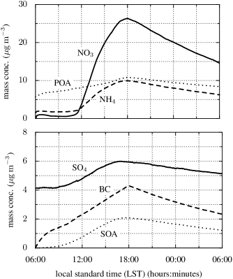
Figure 2: Time series of mass concentrations of selected aerosol species: nitrate ($\rm NO_{3}$), ammonium ($\rm NH_{4}$), POA, sulfate ($\rm SO_{4}$), BC, and SOA. Particle and gas phase emissions were present from 06:00 to 18:00 LST.

Figure 2 shows time series of the bulk aerosol mass concentrations as they result from this urban plume scenario. We observed a pronounced production of ammonium nitrate, reaching nitrate mass concentration of up to $26\rm\,\mu g\,m^{-3}$ and ammonium mass concentration of $10\rm\,\mu g\,m^{-3}$ in the late afternoon. Sulfate mass concentrations increased from $4.1\rm\,\mu g\,m^{-3}$ to $6.0\rm\,\mu g\,m^{-3}$ due to condensation of photochemically produced sulfuric acid. POA and BC were directly emitted (with a temporally constant rate) and accumulated to $11\rm\,\mu g\,m^{-3}$ and $4.3\rm\,\mu g\,m^{-3}$, respectively, until 18:00 LST when the emissions stopped. After 18:00 LST the mass concentrations declined due to dilution, especially nitrate and BC for which the background mass concentration were zero.

3.1 Characterizing mixing state

To characterize the mixing state and to discuss the composition of a particle, we refer to the BC mass fractions as

$$w_{\rm BC,dry} =\frac{\mu_{\rm BC}}{\mu_{\rm dry}}$$ (1)

where $\mu_{\rm BC}$ is the mass of BC in a given particle and $\mu_{\rm dry}$ is the total dry mass.

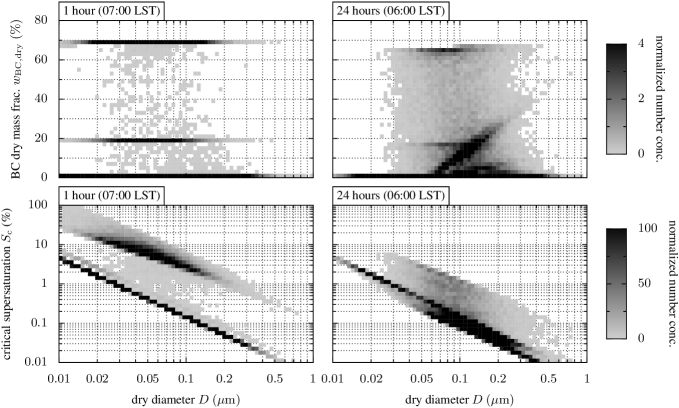
Figure 3: Normalized two-dimensional number distributions after 1 hour (07:00 LST) and 24 hours (06:00 LST the next day) of simulation. The top panels show the normalized value of the two-dimensional distribution $\partial^{2}N_{\rm BC,dry}(D,w)/(\partial\log_{10}D\ \partial w)$ with respect to diameter $D$ and BC dry mass fraction $w_{\rm BC,dry}$, while the bottom panels show the normalized value of the two-dimensional distribution $\partial^{2}N_{\rm S}(D,S_{\rm c})/(\partial\log_{10}D\ \partial\log_{10}S_{\rm c})$ with respect to diameter $D$ and critical supersaturation $S_{\rm c}$.

Based on this quantity, we then define a two-dimensional number concentration that is a function of both particle composition and diameter. The two-dimensional cumulative number distribution $N_{\rm BC,dry}(w,D)$ is the number of particles per volume that have a diameter less than $D$ and a BC mass fraction of less than $w$. The top panels in Figure 3 show the corresponding two-dimensional distributions, normalized with the respective total number concentrations, after 1 hour and after 24 hours of simulation time. Since even at the time of emission no particles were pure BC, particles were not present at $w_{{\rm BC},{\rm dry}}=100\%$. Fresh emissions from diesel vehicles ($w_{{\rm BC},{\rm dry}}=70\%$) and gasoline vehicles ($w_{{\rm BC},{\rm dry}}=20\%$) appear as horizontal lines since particles in one emission category were all emitted with the same composition. At $w_{{\rm BC},{\rm dry}}=0\%$ all the particles appear that do not contain any BC (i.e. background particles and particles from meat cooking emissions that have not undergone coagulation with particles containing BC). After 1 hour (07:00 LST) a small number of particles between these three classes indicate the occurrence of coagulation. Comparing this result to the result for the end of the simulation, we note that at the end of the simulation particles with diameter below $D=0.03\rm\,\mu m$ were heavily depleted due to coagulation. A continuum of mixing states formed between the extreme mixing states of $w_{{\rm BC},{\rm dry}}=0\%$ and $w_{{\rm BC},{\rm dry}}=70\%$.

3.2 Calculating CCN activity

Given that we track the composition evolution of each individual particle throughout the simulation, we can calculate the critical supersaturation $S_{{\rm c}}$ that the particle needs in order to activate. We use the concept of a dimensionless hygroscopicity parameter suggested by Ghan et al. (2001) or Petters and Kreidenweis (2007). In Petters and Kreidenweis (2007) this parameter is denoted by $\kappa$, and we adopt their notation for the remainder of the paper. This concept has the advantage that results from laboratory measurements can be used to quantify the hygroscopicity of complex compounds for which $\kappa$ values cannot be calculated in a straightforward manner. The overall $\kappa$ for a particle is the volume-weighted average of the $\kappa$ values of the constituent species. This requires the assignment of individual $\kappa$ values for each aerosol component in MOSAIC.

Petters and Kreidenweis (2007) compiled a table (Table 1 in their paper) with $\kappa$ values for a variety of inorganic and organic species based on recent laboratory measurements or on thermodynamic model calculations. For $\rm(NH_{4})_{2}SO_{4}$ and $\rm NH_{4}NO_{3}$ they report $\kappa$ values of 0.61 and 0.67, based on calculations by Clegg et al. (1998) and measurements by Svenningsson et al. (2006), respectively. Based on this we assume $\kappa=0.65$ for all salts formed from the $\rm NH_{4}^{+}$-$\rm SO_{4}^{2-}$-$\rm NO_{3}^{-}$ system. For all MOSAIC model species that represent SOA we assume $\kappa=0.1$, based on measurements by Prenni et al. (2007). Following Petters et al. (2006) we assume $\kappa=0.001$ for POA and $\kappa=0$ for BC. The critical supersaturation $S_{\rm c}$ for a particle of diameter $D$ and volume-weighted hygroscopicity parameter $\kappa$ is then given by

$$S_{\rm c}=\frac{C}{\sqrt{\kappa D^{3}}},$$ (2)

where

$$C=\sqrt{\frac{4A^{3}}{27}}\qquad{\rm and}\qquad A=\frac{4\sigma_{w}m_{w}}{R^{*}T\rho_{w}},$$ (3)

with $\sigma_{w}$ being the surface tension of water, $m_{w}$ the molecular weight of water, $R^{*}$ the universal gas constant, $\rho_{w}$ the water density, and $T$ the temperature.

Similarly to the use of $w_{\rm BC,dry}$ above, we can use $S_{\rm c}$ to define a two-dimensional cumulative number distribution $N_{\rm S}(D,S_{\rm c})$ in terms of size and critical supersaturation. The bottom panels in Figure 3 show examples of the corresponding two-dimensional distributions after 1 hour (left) and after 24 hours (right) of simulation. While freshly emitted diesel, gasoline and meat cooking particles differ in their BC and POA mass fractions, they are very similar in their hygroscopicity with initial $\kappa$ values close to zero. After 1 hour they are visible as the dark band of high number concentrations at high $S_{c}$ values. Separated from this we see another dark band representing the most hygroscopic particles, consisting of wet background particles. They contain the largest fraction of inorganic mass (ammonium, sulfate, and nitrate), hence their critical supersaturation is lowest at a given size compared to the other particle classes.

Directly slightly above the most hygroscopic band at 1 hour is a weaker band, which represents the dry background particles. Because they are dry and the vapor pressure of $\rm HNO_{3}$ is still low, nitrate formation does not occur on these particles. The coexistence of wet and dry particles can be explained by the fact that the relative humidity falls below 85% at 06:42 LST, which is the deliquescence point of the inorganic mixture of ammonium, sulfate, and nitrate. Particles that exist before that time contain water and take up nitrate. They stay wet throughout the whole day as a result of the hysteresis of particle deliquescence and crystallization. Particles that are emitted after 06:42 LST do not contain water and take up nitrate only much later. Hence after 1 hour of simulation, at a given size the fraction of highly hygroscopic inorganics is higher for the wet particles, which results in a higher $\kappa$ value and lower critical supersaturation $S_{c}$.

The individual bands are not completely separated at 1 hour, but the regions in between have started to fill out. The reason for this is the occurance of coagulation, which produces particles of intermediate composition and hence corresponding intermediate $S_{\rm c}$ values. After 24 hours the population as a whole has moved to lower critical supersaturations, and the distribution with respect to $S_{\rm c}$ has become more continuous. Given a certain size, the critical supersaturation ranges over about one order of magnitude.

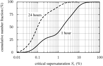
Figure 4: Cloud condensation nuclei spectra after 1 hour (07:00 LST) and 24 hours (06:00 LST the next day) of simulation based on the simulation results shown in Figure 3.

Figure 4 shows CCN properties as more traditional CCN spectra. This representation is the one-dimensional projection of the bottom panels of Figure 3 onto the critical supersaturation axis, plotted as a cumulative distribution. The change in CCN properties over the course of 24 hours is obvious. After 1 hour a supersaturation of $S=1.5\%$ is necessary to activate $50\%$ of the particles by number. This required supersaturation decreases to $S=0.1\%$ after 24 hours. In the following section we use the results of this urban plume scenario as a basis for estimating the aging time-scales.

4 First-order Models of Aging

In this section we describe the first-order model of black carbon aging to which we fit the particle-resolved data simulated with PartMC-MOSAIC, in order to determine the aging time-scale. We emphasize that we do not actually simulate using the first-order models presented in this section. Such first-order systems are frequently used, however, to model the conversion from hydrophobic to hydrophilic black carbon with the single parameter of aging rate or its inverse, the aging time-scale $\tau$ (Croft et al., 2005). More specifically, the aging time-scale represents the time-scale on which particles that would initially not activate turn into particles that can be activated, given a certain chosen supersaturation threshold. Budget equations for the fresh and aged populations can be formulated in terms of either number or mass. A number based aging time-scale is relevant for aerosol indirect forcing as the cloud optical properties depend on the cloud droplet number distribution. On the other hand, a mass aging time-scale is relevant for in-cloud scavenging and wet removal of BC mass. In the following we will present results for both number- and mass-based aging time-scales.

At time $t$, the total number concentration $N_{\rm BC}(t)$ of BC-particles is the sum of the number concentration of BC-containing fresh particles $N_{\rm f}(t)$ and the number concentration of BC-containing aged particles $N_{\rm a}(t)$. We define analogously the total BC mass concentration $M_{\rm BC}(t)$, the BC mass concentration in fresh BC-containing particles $M_{\rm f}(t)$, and the BC mass concentration in aged BC-containing particles $M_{\rm a}(t)$. The aged and fresh populations are separated by applying an aging criterion, in our case activation at a certain supersaturation threshold $S_{\rm c}$. Fresh particles are those with critical supersaturation above the threshold value, while aged particles have critical supersaturations below the threshold.

In the PartMC model we explicitly track a finite number of particles in a computational volume $V$. The number of fresh and aged BC-containing particles in the volume $V(t_{k})$ at time $t_{k}$ is denoted by $n_{\rm f}(t_{k})$ and $n_{\rm a}(t_{k})$, respectively. Similarly, $m_{\rm f}(t_{k})$ and $m_{\rm a}(t_{k})$ are respectively the total mass of BC in fresh and aged BC-containing particles in $V(t_{k})$. The number and mass concentrations of fresh BC-containing particles in $V(t_{k})$ are then given by

$$N_{\rm f}(t_{k}) =\frac{n_{\rm f}(t_{k})}{V(t_{k})} \qquad M_{\rm f}(t_{k}) =\frac{m_{\rm f}(t_{k})}{V(t_{k})}$$ (4)

$$N_{\rm a}(t_{k}) =\frac{n_{\rm a}(t_{k})}{V(t_{k})} M_{\rm a}(t_{k}) =\frac{m_{\rm a}(t_{k})}{V(t_{k})}.$$

The fresh and aged number and mass concentrations can change due to emission and dilution, while condensation and coagulation can transfer number and mass concentration from the fresh to the aged population and vice versa. Changes in number and mass concentrations also occur due to temperature and pressure changes. In our model we neglect at present the impact of heterogeneous reactions on the surface of the particles, although studies have shown that these also contribute to the aging process (Rudich et al., 2007). The gain and loss terms for the fresh and aged BC-containing populations are given in Table 2.

To express changes in number and mass for coagulation we consider that all constituent particles are lost during a coagulation event and the product of coagulation is a gain of a new particle. Table 3 shows the overview of all possible combinations and the resulting terms for each of those combinations. For example, let us assume that there are four independent coagulation events within a single timestep: one event between two fresh BC-containing particles resulting in an aged particle, two events between fresh and aged BC-containing particles each resulting in an aged particle, and one event between a fresh BC-containing particle and a non-BC-containing particle resulting in a fresh particle. Then we have losses $\Delta n^{\rm coag}_{\rm f\to a}(t_{k-1},t_{k})=5$ and $\Delta n^{\rm coag}_{\rm a\to a}(t_{k-1},t_{k})=2$, and gains $\Delta n^{\rm coag}_{\rm f}(t_{k-1},t_{k})=1$ and $\Delta n^{\rm coag}_{\rm a}(t_{k-1},t_{k})=3$.

Note that for each particle pairing in Table 3 there can be two outcomes. For example, coagulation of a small fresh and large aged particle generally produces an aged particle, while coagulation of large fresh and small aged generally produces a fresh particle. When $S_{c}$, as calculated in equations (2)–(3), is used as the criterion for fresh versus aged, it can be shown that coagulation of two aged particles never produces a fresh particle, and that the coagulation of two fresh particles with $S_{c}$ values close to the cutoff value can produce an aged particle.

Coagulation can result in a net loss of number but must conserve mass. We thus have

$$\dot{N}^{\rm coag}_{\rm a}(t) \leq\dot{N}^{\rm coag}_{\rm f\to a}(t)+\dot{N}^{\rm coag}_{\rm a\to a}(t)$$ (5)

$$\dot{M}^{\rm coag}_{\rm a}(t) =\dot{M}^{\rm coag}_{\rm f\to a}(t)+\dot{M}^{\rm coag}_{\rm a\to a}(t)$$ (6)

$$\Delta n^{\rm coag}_{\rm a}(t_{k-1},t_{k}) \leq\Delta n^{\rm coag}_{\rm f\to a}(t_{k-1},t_{k})+\Delta n^{\rm coag}_{\rm a\to a}(t_{k-1},t_{k})$$ (7)

$$\Delta m^{\rm coag}_{\rm a}(t_{k-1},t_{k}) =\Delta m^{\rm coag}_{\rm f\to a}(t_{k-1},t_{k})+\Delta m^{\rm coag}_{\rm a\to a}(t_{k-1},t_{k})$$ (8)

and similarly for coagulation resulting in fresh particles.

The following continuous equations describe the evolution of the number and mass concentrations of fresh and aged BC-containing populations:

$$\frac{dN_{\rm f}(t)}{dt} =\dot{N}^{\rm density}_{\rm f}(t)+\dot{N}^{\rm emit}_{\rm f}(t)-\dot{N}^{\rm dilution}_{\rm f}(t)$$ (9)

$$\qquad+\dot{N}^{\rm cond}_{\rm a\to f}(t)+\dot{N}^{\rm coag}_{\rm f}(t)-\dot{N}^{\rm coag}_{\rm f\to f}(t)-\underbrace{\Bigl{(}\dot{N}^{\rm cond}_{\rm f\to a}(t)+\dot{N}^{\rm coag}_{\rm f\to a}(t)\Bigr{)}}_{\dot{N}^{\rm aging}(t)}$$

$$\frac{dN_{\rm a}(t)}{dt} =\dot{N}^{\rm density}_{\rm a}(t)+\dot{N}^{\rm emit}_{\rm a}(t)-\dot{N}^{\rm dilution}_{\rm a}(t)$$ (10)

$$\qquad+\dot{N}^{\rm cond}_{\rm f\to a}(t)+\dot{N}^{\rm coag}_{\rm a}(t)-\dot{N}^{\rm coag}_{\rm a\to a}(t)-\underbrace{\Bigl{(}\dot{N}^{\rm cond}_{\rm a\to f}(t)+\dot{N}^{\rm coag}_{\rm a\to f}(t)\Bigr{)}}_{\dot{N}^{\text{de-aging}}(t)}$$

$$\frac{dM_{\rm f}(t)}{dt} =\dot{M}^{\rm density}_{\rm f}(t)+\dot{M}^{\rm emit}_{\rm f}(t)-\dot{M}^{\rm dilution}_{\rm f}(t)$$ (11)

$$\qquad+\underbrace{\Bigl{(}\dot{M}^{\rm cond}_{\rm a\to f}(t)+\dot{M}^{\rm coag}_{\rm a\to f}(t)\Bigr{)}}_{\dot{M}^{\rm de-aging}(t)}-\underbrace{\Bigl{(}\dot{M}^{\rm cond}_{\rm f\to a}(t)+\dot{M}^{\rm coag}_{\rm f\to a}(t)\Bigr{)}}_{\dot{M}^{\rm aging}(t)}$$

$$\frac{dM_{\rm a}(t)}{dt} =\dot{M}^{\rm density}_{\rm a}(t)+\dot{M}^{\rm emit}_{\rm a}(t)-\dot{M}^{\rm dilution}_{\rm a}(t)$$ (12)

$$\qquad+\underbrace{\Bigl{(}\dot{M}^{\rm cond}_{\rm f\to a}(t)+\dot{M}^{\rm coag}_{\rm f\to a}(t)\Bigr{)}}_{\dot{M}^{\rm aging}(t)}-\underbrace{\Bigl{(}\dot{M}^{\rm cond}_{\rm a\to f}(t)+\dot{M}^{\rm coag}_{\rm a\to f}(t)\Bigr{)}}_{\dot{M}^{\rm de-aging}(t)}$$

Note that the mass equations (11)–(12) have been simplified from forms identical to the number equations (9)–(10) by using equation (6) for the conservation of mass during coagulation. Condensation (or rather evaporation) and coagulation can in principle also produce a transfer from aged to fresh particles. This is reflected by the terms denoted as $\dot{N}^{\rm de-aging}(t)$ and $\dot{M}^{\rm de-aging}(t)$ above.

The aging time-scales $\tau_{\rm N}$ and $\tau_{\rm M}$ for number and mass are then determined by the first-order models:

$$\dot{N}^{\rm aging}(t) =\frac{1}{\tau_{\rm N}(t)}N_{\rm f}(t)$$ (13)

$$\dot{M}^{\rm aging}(t) =\frac{1}{\tau_{\rm M}(t)}M_{\rm f}(t)$$ (14)

The discrete versions of the balance equations (9)–(12) are:

$$n_{\rm f}(t_{k})-n_{\rm f}(t_{k-1}) =\Delta n^{\rm emit}_{\rm f}(t_{k-1},t_{k})-\Delta n^{\rm dilution}_{\rm f}(t_{k-1},t_{k})$$ (15)

$$\qquad+\Delta n^{\rm cond}_{\rm a\to f}(t_{k-1},t_{k})+\Delta n^{\rm coag}_{\rm f}(t_{k-1},t_{k})-\Delta n^{\rm coag}_{\rm f\to f}(t_{k-1},t_{k})$$

$$\qquad-\underbrace{\Bigl{(}\Delta n^{\rm cond}_{\rm f\to a}(t_{k-1},t_{k})+\Delta n^{\rm coag}_{\rm f\to a}(t_{k-1},t_{k})\Bigr{)}}_{\Delta n^{\rm aging}(t_{k-1},t_{k})}$$

$$n_{\rm a}(t_{k})-n_{\rm a}(t_{k-1}) =\Delta n^{\rm emit}_{\rm a}(t_{k-1},t_{k})-\Delta n^{\rm dilution}_{\rm a}(t_{k-1},t_{k})$$ (16)

$$\qquad+\Delta n^{\rm cond}_{\rm f\to a}(t_{k-1},t_{k})+\Delta n^{\rm coag}_{\rm a}(t_{k-1},t_{k})-\Delta n^{\rm coag}_{\rm a\to a}(t_{k-1},t_{k})$$

$$\qquad-\underbrace{\Bigl{(}\Delta n^{\rm cond}_{\rm a\to f}(t_{k-1},t_{k})+\Delta n^{\rm coag}_{\rm a\to f}(t_{k-1},t_{k})\Bigr{)}}_{\Delta n^{\rm de-aging}(t_{k-1},t_{k})}$$

$$m_{\rm f}(t_{k})-m_{\rm f}(t_{k-1}) =\Delta m^{\rm emit}_{\rm f}(t_{k-1},t_{k})-\Delta m^{\rm dilution}_{\rm f}(t_{k-1},t_{k})$$ (17)

$$\qquad+\underbrace{\Bigl{(}\Delta m^{\rm cond}_{\rm a\to f}(t_{k-1},t_{k})+\Delta m^{\rm coag}_{\rm a\to f}(t_{k-1},t_{k})\Bigr{)}}_{\Delta m^{\rm de-aging}(t_{k-1},t_{k})}$$

$$\qquad-\underbrace{\Bigl{(}\Delta m^{\rm cond}_{\rm f\to a}(t_{k-1},t_{k})+\Delta m^{\rm coag}_{\rm f\to a}(t_{k-1},t_{k})\Bigr{)}}_{\Delta m^{\rm aging}(t_{k-1},t_{k})}$$

$$m_{\rm a}(t_{k})-m_{\rm a}(t_{k-1}) =\Delta m^{\rm emit}_{\rm a}(t_{k-1},t_{k})-\Delta m^{\rm dilution}_{\rm a}(t_{k-1},t_{k})$$ (18)

$$\qquad+\underbrace{\Bigl{(}\Delta m^{\rm cond}_{\rm f\to a}(t_{k-1},t_{k})+\Delta m^{\rm coag}_{\rm f\to a}(t_{k-1},t_{k})\Bigr{)}}_{\Delta m^{\rm aging}(t_{k-1},t_{k})}$$

$$\qquad-\underbrace{\Bigl{(}\Delta m^{\rm cond}_{\rm a\to f}(t_{k-1},t_{k})+\Delta m^{\rm coag}_{\rm a\to f}(t_{k-1},t_{k})\Bigr{)}}_{\Delta m^{\rm de-aging}(t_{k-1},t_{k})}$$

Here equation (8) for the discrete conservation of mass during coagulation was used to simplify the mass equations, as in the continuous case.

By comparing the continuous equations (9)– (12) to the discrete equations (15)– (18) using the relationships (4) we see that the continuous aging terms can be approximated by:

$$\dot{N}^{\rm aging}(t_{k}) \approx\frac{\Delta n^{\rm aging}(t_{k-1},t_{k})}{(t_{k}-t_{k-1})V(t_{k})}$$ (19)

$$\dot{M}^{\rm aging}(t_{k}) \approx\frac{\Delta m^{\rm aging}(t_{k-1},t_{k})}{(t_{k}-t_{k-1})V(t_{k})},$$ (20)

where the use of $V$ at time $t_{k}$ is because the computational volume $V$ is updated first within each timestep in the PartMC algorithm (Riemer et al., 2009, Figure 1).

From equations (13) and (14) and the relationships (4), the aging time-scales $\tau_{\rm N}$ and $\tau_{\rm M}$ are then approximated by:

$$\tau_{\rm N}(t_{k}) \approx\frac{(t_{k}-t_{k-1})n_{\rm f}(t_{k})}{\Delta n^{\rm aging}(t_{k-1},t_{k})}$$ (21)

$$\tau_{\rm M}(t_{k}) \approx\frac{(t_{k}-t_{k-1})m_{\rm f}(t_{k})}{\Delta m^{\rm aging}(t_{k-1},t_{k})}.$$ (22)

For the analysis in Section 5 we additionally define the aging time-scale $\tau_{\rm N}^{\rm cond}$ ignoring the impact of coagulation, an average time-scale $\tau_{\rm N,day}$ during the day, and an average time-scale $\tau_{\rm N,night}$ during the night, given by:

$$\tau_{\rm N}^{\rm cond}(t_{k}) \approx\frac{(t_{k}-t_{k-1})n_{\rm f}(t_{k})}{\Delta n^{\rm cond}_{\rm f\to a}(t_{k-1},t_{k})}$$ (23)

$$(\tau_{\rm N,day})^{-1} =\frac{1}{3\,{\rm hours}}\int_{\rm 12:00\,LST}^{\rm 15:00\,LST}\bigl{(}\tau_{\rm N}(t)\bigr{)}^{-1}\,dt$$ (24)

$$(\tau_{\rm N,night})^{-1} =\frac{1}{10\,{\rm hours}}\int_{\rm 18:00\,LST}^{\rm 04:00\,LST}\bigl{(}\tau_{\rm N}(t)\bigr{)}^{-1}\,dt,$$ (25)

and similarly for $\tau_{\rm M}^{\rm cond}$, $\tau_{\rm M,day}$, $\tau_{\rm M,night}$, $\tau_{\rm N,day}^{\rm cond}$, and so on.

5 Results

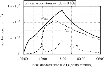
Figure 5: Time series of total number concentration $N_{\rm BC}$ of BC-containing particles and number concentrations $N_{\rm f}$ and $N_{\rm a}$ for fresh and aged BC-containing particles, respectively. The critical supersaturation separating fresh and aged particles is set to $S_{\rm c}=0.6\%$.

In this section we show results for supersaturation thresholds ranging between $S_{\rm c}=0.1\%$ and $S_{\rm c}=1.0\%$, as these are typically achieved in updrafts in stratus and cumulus clouds (Warner, 1968). To limit the number of figures we use $S_{\rm c}=0.6\%$ as a base case. Figure 5 shows the time series for $N_{\rm f}$, $N_{\rm a}$, and $N_{\rm BC}=N_{\rm f}+N_{\rm a}$ for $S_{\rm c}=0.6\%$. The total number concentration $N_{\rm BC}$ of BC-containing particles increased until 18:00 LST due to the emission of particles. After the emissions stopped, $N_{\rm BC}$ decreased as a result of continued dilution and coagulation. The time series for $N_{\rm f}$ and $N_{\rm a}$ show that both increased in the morning hours. A pronounced transfer from fresh to aged occurred after 11:30 LST, the time when nitrate formation started taking place on the dry particles (compare Figure 2). This process efficiently contributed to the conversion of fresh particles to aged particles, which was reflected by a short aging time-scale.

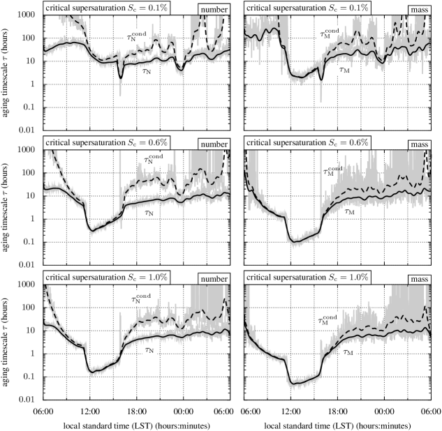
Figure 6: Comparison of aging time-scales based on number (left) and mass (right), showing both the time-scales due to condensation and coagulation ($\tau_{\rm N}$ and $\tau_{\rm M}$) and the time-scales due to condensation alone ($\tau_{\rm N}^{\rm cond}$ and $\tau_{\rm M}^{\rm cond}$). The top panels have the critical supersaturation separating fresh from aged particles set to $S_{\rm c}=0.1\%$, while the middle panels have $S_{\rm c}=0.6\%$, and the bottom panels have $S_{\rm c}=1.0\%$.

The left column of Figure 6 compares the aging time-scales $\tau_{\rm N}$ and $\tau_{\rm N}^{\rm cond}$ computed according to equations (21) and (23) for different supersaturation thresholds. The top, middle and bottom panels shows the results for supersaturation thresholds $S_{\rm c}=0.1\%$, $S_{\rm c}=0.6\%$, and $S_{\rm c}=1\%$, respectively. The grey shading is the raw data, and the black lines are results computed from smoothing the transfer rates with a Hann filter with a window width of 1 hour.

The solid lines represent $\tau_{\rm N}$, including the contributions due to both coagulation and condensation according to equation (21). For $S_{\rm c}=0.6\%$, $\tau_{\rm N}$ started off in the morning with values of $\tau_{\rm N}\approx 20$ hours. It decreased sharply after 11:00 LST, which is the time when photochemistry was at its peak, and nitrate formation was most pronounced, hence leading to a fast aging process. Between 12:00 LST and 16:00 LST, $\tau_{\rm N}$ was less than 1 hour, and reached values as low as 0.2 hours. After 16:00 LST, as photochemistry slowed down, $\tau_{\rm N}$ increased again, reaching a plateau of $\tau_{\rm N}\approx 10$ hours during the evening and night.

The broken lines represent $\tau_{\rm N}^{\rm cond}$ as defined in equation (23), i.e. the contribution due to coagulation is ignored. There was only a small difference between $\tau_{\rm N}$ and $\tau_{\rm N}^{\rm cond}$ during midday and early afternoon when condensation was operating very effectively. However during morning, afternoon and night, neglecting coagulation lead to larger time-scales (up to one order of magnitude).

A similar pattern was found for $S_{\rm c}=1\%$, shown in the bottom panel. For $S_{\rm c}=0.1\%$ we generally obtained larger time-scales. During the morning, $\tau_{\rm N}$ was about 50 hours and decreased to 10 hours in the early afternoon. There was a short period around 16:00 LST when $\tau_{\rm N}$ dropped to 2 hours. Obviously, at $S_{\rm c}=0.1\%$, even after the growth due to condensation of ammonium nitrate, the particles were still too small to be activated to the same extent as seen for the larger supersaturations. During the following night $\tau_{\rm N}$ was around 10–20 hours. For this low supersaturation the contrast between day and night was not as pronounced as for $S_{\rm c}=0.6\%$ or $S_{\rm c}=1\%$.

Qualitatively, the temporal evolution of $\tau_{\rm M}$ (right column) was similar to the number-based result $\tau_{\rm N}$. However the day/night contrast was more pronounced for the case with $S_{\rm c}=0.1\%$, and the time-scales based on mass during the day were lower than the ones based on number.

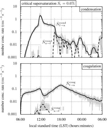
Figure 7: Transfer rates due to condensation (top) and coagulation (bottom). The critical supersaturation separating fresh and aged particles is set to $S_{\rm c}=0.6\%$. The notation is according to Table 2.

Figure 7 shows the individual transfer terms of BC-containing particles for the case $S_{\rm c}=0.6\%$. The transfer rate $\dot{N}_{\rm a\to f}^{\rm coag}$ due to coagulation from aged to fresh was very small throughout the whole day, remaining below $0.01$ $\rm cm^{-3}\,s^{-1}$. The transfer rate $\dot{N}_{\rm f\to a}^{\rm coag}$ due to coagulation from fresh to aged followed the time series of $N_{\rm f}$. The minimum of $N_{\rm f}$ during the early afternoon was reflected in a minimum of the transfer rate $\dot{N}_{\rm f\to a}^{\rm coag}$. The transfer rate $\dot{N}_{\rm f\to a}^{\rm cond}$ due to condensation from fresh to aged was large between 11:30 and 15:00 LST, consistent with the decrease of $\tau_{\rm N}$ in Figure 6. Lastly, there was a non-zero transfer $\dot{N}_{\rm a\to f}^{\rm cond}$ from aged to fresh due to condensation, which was larger than $\dot{N}_{\rm f\to a}^{\rm cond}$ towards the end of the simulation. This was related to a shrinking of the particles due to decreasing relative humidity (compare Figure 1).

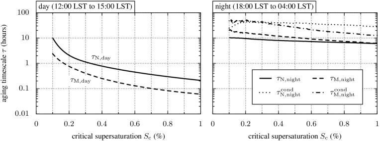
Figure 8: Day (left) and night (right) averages of the aging time-scale, as defined in equations (23)–(25). As can be see from Figure 6, during the day the condensation-induced aging dominates, so $\tau^{\rm cond}_{\rm N,day}$ is almost indistinguishable from $\tau_{\rm N,day}$, and similarly for mass.

Figure 8 summarizes the results for the different aging time-scale definitions. We calculated $\tau_{\rm N,day}$ and $\tau_{\rm N,night}$ according to equation (23) for several hundred different supersaturation thresholds between $S_{\rm c}=0.1\%$ and $S_{\rm c}=1\%$. We also distinguished between the definition of $\tau$ including the transfer due to coagulation and condensation (solid lines), and including only the transfer due to condensation, $\tau_{\rm N,day}^{\rm cond}$ and $\tau_{\rm N,night}^{\rm cond}$ (broken lines).

For this particular urban plume scenario the following general features emerge: during the day, condensation of semi-volatile species, in our case especially ammonium nitrate, was the dominant process for aging. The time-scales based on number were larger than the time-scales based on mass during the day, by roughly a factor of five. The aging time-scales had a strong dependence on supersaturation threshold. For $S_{\rm c}=0.1\%$, $\tau_{\rm N,day}$ was 10 hours, whereas for $S_{\rm c}=1\%$, $\tau_{\rm N,day}$ was only 0.2 hours. During the night condensation was limited, hence coagulation was the dominant aging process. For low supersaturation thresholds, the time-scales based on number were smaller than the time-scales based on mass, but this difference decreased for higher supersaturation thresholds.

6 Conclusions

In this paper we presented a method for explicitly calculating aging time-scales of black carbon aerosol using particle-resolved model simulations with PartMC-MOSAIC. We developed number-based and mass-based aging time-scales using the activation of the particles at a given supersaturation as a criterion for aging. We applied this method to an urban plume scenario (Riemer et al., 2009) for a range of supersaturation thresholds between 0.1% and 1% and considered condensation of secondary substances and coagulation as aging mechanisms. Aging due to heterogeneous processes (chemical aging) were not included.

For this particular scenario we found a separation into day and night regimes. During the day the condensation-induced aging dominated, in particular due to the formation of ammonium nitrate. Therefore the condensation-only number-based aging time-scale $\tau_{\rm N,day}^{\rm cond}$ was almost the same as the total time-scale $\tau_{\rm N,day}$ and similarly for mass. The daytime aging number-based time-scale $\tau_{\rm N,day}$ was about 10 hours for a supersaturation threshold of $S_{\rm c}=0.1\%$ and decreased to 0.06 hours for a threshold of $S_{\rm c}=1\%$. The daytime mass-based aging time-scale $\tau_{\rm M,day}$ was about a factor of five lower than $\tau_{\rm N,day}$ for all supersaturation thresholds.

During the night, the absence of condensable species caused the number-based aging time-scale $\tau_{\rm N,night}$ to be about one order of magnitude larger than during the day. Coagulation became dominant, which was reflected by the fact that the condensation-only time-scale $\tau_{\rm N,night}^{\rm cond}$ was an order of magnitude larger than the total time-scale $\tau_{\rm N,night}$. The nighttime aging time-scales therefore depended on the particle number concentrations. We suspect that chemical aging would have its largest impact during periods when condensation is not dominant, i.e. during the night in our case.

Compared to the time-scales used in global models, which are typically on the order of 30 hours (Chung and Seinfeld, 2002; Koch, 2001, e.g.), our time-scales were much shorter, in particular during the day. This confirmed findings by Riemer et al. (2004) who showed with a completely different approach that daytime and nighttime aging regimes exists, and that aging during the day proceeds very rapidly.

However some caveats need to be emphasized: our urban plume scenario represents only one scenario, with very polluted conditions and fairly high number concentrations during the night ($N_{\rm BC}\approx 5000$ $\rm cm^{-3}$). For lower number concentrations, we expect the aging time-scales during the night to increase.

Acknowledgments.

Funding for N. Riemer and M. West was provided by the National Science Foundation (NSF) under grant ATM 0739404. Funding for R. A. Zaveri and R. C. Easter was provided by the Aerosol-Climate Initiative as part of the Pacific Northwest National Laboratory (PNNL) Laboratory Directed Research and Development (LDRD) program. Pacific Northwest National Laboratory is operated for the U.S. Department of Energy by Battelle Memorial Institute under contract DE-AC06-76RLO 1830.

Initial/Background	$N$ ($\rm m^{-3}$)	$D_{\rm gn}$ ($\rm\mu m$)	$\sigma_{\rm g}$ (1)	Composition by mass
Aitken Mode	$3.2\cdot 10^{9}$	0.02	1.45	50% $\rm(NH_{4})_{2}SO_{4}$, 50% POA
Accumulation Mode	$2.9\cdot 10^{9}$	0.116	1.65	50% $\rm(NH_{4})_{2}SO_{4}$, 50% POA
Emissions	$E$ ($\rm m^{-2}\,s^{-1}$)	$D_{\rm gn}$ ($\rm\mu m$)	$\sigma_{\rm g}$ (1)	Composition by mass
Meat cooking	$9\cdot 10^{6}$	0.086	1.9	100% POA
Diesel vehicles	$1.6\cdot 10^{8}$	0.05	1.7	30% POA, 70% BC
Gasoline vehicles	$5\cdot 10^{7}$	0.05	1.7	80% POA, 20% BC

Table 1: Initial and emitted aerosol distribution parameters. The initial aerosol distribution is also used as the background aerosol distribution. The percentages for the composition are by mass. $E$ is the area source strength of particle emissions. Dividing $E$ by the mixing height and multiplying by a normalized composition distribution gives the number distribution emission rate.

Terms	Description
$N_{\rm f}(t)$, $N_{\rm a}(t)$	Number concentration of fresh/aged BC-containing particles.
$\dot{N}^{\rm emit}_{\rm f}(t)$, $\dot{N}^{\rm emit}_{\rm a}(t)$	Gain rate of number concentration of fresh/aged BC-containing particles due to emission.
$\dot{N}^{\rm dilution}_{\rm f}(t)$, $\dot{N}^{\rm dilution}_{\rm a}(t)$	Loss rate of number concentration of fresh/aged BC-containing particles due to dilution.
$\dot{N}^{\rm cond}_{\rm f\to a}(t)$, $\dot{N}^{\rm cond}_{\rm a\to f}(t)$	Gain rate of number concentration of aged/fresh BC-containing particles due to condensation or evaporation on fresh/aged particles.
$\dot{N}^{\rm coag}_{\rm f}(t)$, $\dot{N}^{\rm coag}_{\rm a}(t)$	Gain rate of number concentration of fresh/aged BC-containing particles from coagulation events.
$\dot{N}^{\rm coag}_{\rm f\to f}(t)$, $\dot{N}^{\rm coag}_{\rm f\to a}(t)$	Loss rate of number concentration of fresh BC-containing particles to coagulation events resulting in fresh/aged particles.
$\dot{N}^{\rm coag}_{\rm a\to a}(t)$, $\dot{N}^{\rm coag}_{\rm a\to f}(t)$	Loss rate of number concentration of aged BC-containing particles to coagulation events resulting in aged/fresh particles.
$\dot{N}^{\rm density}_{\rm f}(t)$, $\dot{N}^{\rm density}_{\rm a}(t)$	Gain rate of number concentration of fresh/aged BC-containing particles due to air density changes.
$\dot{N}^{\rm aging}(t)$, $\dot{N}^{\rm de-aging}(t)$	Net transfer rate of fresh-to-aged/aged-to-fresh number concentration of BC-containing particles.

Table 2: Description of individual terms in equations (9) and (10). With the exception of $\dot{N}^{\rm density}_{\rm f}(t)$ and $\dot{N}^{\rm density}_{\rm a}(t)$ all of these terms must be non-negative. The same notation is for the terms in equations (11) and (12) for mass concentration, and for the corresponding discrete equations (15)–(18). The discrete terms are expressed as a change in number or mass within a timestep, so that $\Delta n^{\rm cond}_{\rm f\to a}(t_{k-1},t_{k})$ is the number of BC-containing particles in the computational volume that change from fresh to aged due only to condensation during the timestep from time $t_{k-1}$ to $t_{k}$, for example. There are no discrete terms for air density changes as they are incorporated by changing the computational volume $V$.

Particle 1	Particle 2	Resulting particle	Non-zero loss terms	Non-zero gain terms
fresh	fresh	fresh	$\Delta n^{\rm coag}_{\rm f\to f}=2$	$\Delta n^{\rm coag}_{\rm f}=1$
fresh	fresh	aged	$\Delta n^{\rm coag}_{\rm f\to a}=2$	$\Delta n^{\rm coag}_{\rm a}=1$
aged	fresh	fresh	$\Delta n^{\rm coag}_{\rm a\to f}=1$, $\Delta n^{\rm coag}_{\rm f\to f}=1$	$\Delta n^{\rm coag}_{\rm f}=1$
aged	fresh	aged	$\Delta n^{\rm coag}_{\rm a\to a}=1$, $\Delta n^{\rm coag}_{\rm f\to a}=1$	$\Delta n^{\rm coag}_{\rm a}=1$
aged	aged	aged	$\Delta n^{\rm coag}_{\rm a\to a}=2$	$\Delta n^{\rm coag}_{\rm a}=1$
fresh	non-BC	fresh	$\Delta n^{\rm coag}_{\rm f\to f}=1$	$\Delta n^{\rm coag}_{\rm f}=1$
fresh	non-BC	aged	$\Delta n^{\rm coag}_{\rm f\to a}=1$	$\Delta n^{\rm coag}_{\rm a}=1$
aged	non-BC	fresh	$\Delta n^{\rm coag}_{\rm a\to f}=1$	$\Delta n^{\rm coag}_{\rm f}=1$
aged	non-BC	aged	$\Delta n^{\rm coag}_{\rm a\to a}=1$	$\Delta n^{\rm coag}_{\rm a}=1$

Table 3: The different coagulation events and the resulting expressions for the loss and gain terms of the number of fresh and aged BC-containing particles. Similar expressions exist for mass changes $\Delta m$ in the particle-resolved model and for the number rates $\dot{N}$ and mass rates $\dot{M}$ in the continuous model.

References

- Andreae and Gelencśer (2006) Andreae, M., Gelencśer, A., 2006. Black carbon or brown carbon? The nature of light-absorbing carbonaceous aerosols. Atmos. Chem. Phys. 6, 3131–3148.
- Bond et al. (2004) Bond, T., Streets, D., Yarber, K., Nelson, S., Woo, J., Klimont, Z., 2004. A technology-based global inventory of black and organic carbon emissions from combustion. J. Geophys. Res 109 (D14), D14203.
- Chung and Seinfeld (2002) Chung, S. H., Seinfeld, J. H., 2002. Global distribution and climate forcing of carbonaceous aerosols. J. Geophys. Res. 107.
- Clegg et al. (1998) Clegg, S., Brimblecombe, P., Wexler, A., 1998. Thermodynamic model of the system ------ at 298.15 K. J. Phys. Chem. A 102 (12), 2155–2171.
- Cooke et al. (1999) Cooke, W. F., Liousse, C., Cachier, H., Feichter, J., 1999. Construction of a 1 fossil fuel emission data set for carbonaceous aerosol and implementation and radiative impact in the ECHAM4 model. J. Geophys. Res. 104, 22137–22162.
- Croft et al. (2005) Croft, B., Lohmann, U., von Salzen, K., 2005. Black carbon aging in the Canadian Centre for Climate modelling and analysis atmospheric general circulation model. Atmos. Chem. Phys. 5, 1931–1949, sRef-ID:1680-7324/acp/2005-5-1931.
- Cubison et al. (2008) Cubison, M. J., Ervens, B., Feingold, G., Docherty, K. S., Ulbrich, I. M., Shields, L., Prather, K., Hering, S., Jimenez, J. L., 2008. The influence of chemical composition and mixing state on Los Angeles urban aerosol on CCN number and cloud properties. Atmos. Chem. Phys. Discuss. 8, 5629–5681.
- Eldering and Cass (1996) Eldering, A., Cass, G. R., 1996. Source-oriented model for air pollution effects on visibility. J. Geophys. Res. 101, 19343–19369.
- Furutani et al. (2008) Furutani, H., Dall’osto, M., Roberts, G., Prather, K., 2008. Assessment of the relative importance of atmospheric aging on CCN activity derived from field observations. Atmos. Environ. 42 (13), 3130–3142.
- Ghan et al. (2001) Ghan, S., Laulainen, N., Easter, R., Wagener, R., Nemesure, S., Chapman, E., Zhang, Y., Leung, R., 2001. Evaluation of aerosol direct radiative forcing in MIRAGE. Journal of Geophysical Research 106 (D6), 5317–5334.
- Horvath and Trier (1993) Horvath, H., Trier, A., 1993. A study of the aerosol of Santiago de Chile — I. Light extinction coefficient. Atmos. Environ. 27, 371–384.
- IPCC (2007) IPCC, 2007. Climate Change 2007: The physical science basis summary for policymakes. Contribution of working group I to the fourth assessment report of the Intergovernmental Panel on Climate Change. World Meteorological Organization, Geneva, Switzerland.
- Jaenicke (1993) Jaenicke, R., 1993. Aerosol-Cloud-Climate Interaction. Academic Press, San Diego, CA, Ch. Tropospheric aerosols, pp. 1–31.
- Kittelson et al. (2006a) Kittelson, D., Watts, W., Johnson, J., 2006a. On-road and laboratory evaluation of combustion aerosols — Part 1: Summary of diesel engine results. Aerosol Sci. 37, 913–930.
- Kittelson et al. (2006b) Kittelson, D., Watts, W., Johnson, J., Schauer, J., Lawson, D., 2006b. On-road and laboratory evaluation of combustion aerosols — Part 2: Summary of spark ignition engine results. Aerosol Sci. 37, 931–949.
- Kleeman et al. (2000) Kleeman, M., Schauer, J., Cass, G., 2000. Size and composition distribution of fine particulate matter emitted from motor vehicles. Environ. Sci. Technol. 34, 1132–1142.
- Koch (2001) Koch, D., 2001. Transport and direct radiative forcing of carbonaceous and sulfate aerosols in the GISS GCM. J. Geophys. Res. 106, 20311–20332.
- Lohmann et al. (1999) Lohmann, U., Feichter, J., Chuang, C. C., Penner, J. E., 1999. Prediction of the number of cloud droplets in the ECHAM GCM. J. Geophys. Res. 104, 9169–9198.
- McFiggans et al. (2006) McFiggans, G., Artaxo, P., Baltensperger, U., Coe, H., Facchini, M. C., Feingold, G., Fuzzi, S., Gysel, M., Laaksonen, A., Lohmann, U., Mentel, T. F., Murphy, D. M., O’Dowd, C. D., Snider, J. R., Weingartner, E., 2006. The effect of physical and chemical aerosol properties on warm cloud droplet activation. Atmos. Chem. Phys. 6, 2593–2649.
- McMurry and Stolzenburg (1989) McMurry, P., Stolzenburg, M., 1989. On the sensitivity of particle size to relative humidity for Los Angeles aerosols. Atmospheric Environment (1967) 23 (2), 497–507.
- Medalia and Rivin (1982) Medalia, A., Rivin, D., 1982. Particulate carbon and other components of soot and carbon black. Carbon 20, 481–492.
- Menon et al. (2002) Menon, S., Hansen, J., Nazarenko, L., Luo, Y. F., 2002. Climate effects of black carbon aerosols in China and India. Science 297, 2250–2253.
- Moffet et al. (2008) Moffet, R., Qin, X., Rebotier, T., Furutani, H., Prather, K., 2008. Chemically segregated optical and microphysical properties of ambient aerosols measured in a single-particle mass spectrometer. J. Geophys. Res. 113 (D12), D12213.
- Petters et al. (2006) Petters, M., Prenni, A., Kreidenweis, S., DeMott, P., Matsunaga, A., Lim, Y., Ziemann, P., 2006. Chemical aging and the hydrophobic-to-hydrophilic conversion of carbonaceous aerosol. Geophys. Res. Lett 33, L24806.