Abstract

A detailed derivation of a two dimensional (2D) low energy effective model for spinless fermions on a square lattice with local interactions is given. This derivation utilizes a particular continuum limit that is justified by physical arguments. It is shown that the effective model thus obtained can be treated by exact bosonization methods. It is also discussed how this effective model can be used to obtain physical information about the corresponding lattice fermion system.

1 Introduction

One powerful approach to 1D lattice fermion systems is to utilize a particular continuum limit to derive a low-energy effective model that can be solved analytically. For the simplest case of spinless fermions with local interactions away from half-filling, this approach leads to the so-called Luttinger model [1] which can be solved exactly using bosonization [2]; see [3, 4, 5] for closely related pioneering papers. Exact solubility means a lot in this case: not only the partition function but all Green’s functions of the Luttinger model can be computed exactly by analytical methods; see e.g. [6, 7] and references therein. This method can be generalized to 1D Hubbard-like systems and is the basis of a paradigm for 1D interacting fermion systems [8] (for a textbook presentation see e.g. [9], Sections 29–32). In a previous paper we outlined a similar approach to 2D lattice fermion systems [10]. The aim of this paper is to present details and generalizations of this proposal. Applications and additional results are given elsewhere [11, 12].

Our starting point is the so-called 2D $t$-$t^{\prime}$-$V\,$model describing spinless fermions on a square lattice with nearest-neighbor and next-nearest-neighbor hopping constants $t$ and $t^{\prime}$, respectively, and with nearest-neighbor density-density interaction strength $V/2$; see (20)–(21) for a precise definition. We propose a particular continuum limit similar to one allowing to derive the Luttinger model from the 1D $t$-$t^{\prime}$-$V\,$model. Using that we derive a 2D fermion model that is a natural 2D analogue of the Luttinger model not only by its relation to 2D lattice fermions but also because it can be treated by exact bosonization methods. However, different from the 1D case, we find that only parts of the fermion degrees of freedom of this 2D Luttinger model can be bosonized and thus treated exactly. We suggest to treat the other degrees of freedom by mean field theory, and we argue that there is a significant doping regime where this treatment is adequate. We refer to the fermion degrees of freedom that can be bosonized as nodal and the others as antinodal.

The 2D $t$-$t^{\prime}$-$V\,$model is a spinless variant of the 2D Hubbard model which is often regarded as prototype model for high temperature superconductors (HTSC) [14]. As discussed in Section 3.1, our approach and terminology is partly motivated by the so-called pseudogap in HTSC [15]. Another motivation are mean field theory results about 2D Hubbard-like models; see [16] and references therein. Our approach was also inspired by renormalization group studies of the 2D Hubbard model that predict a truncation of the Fermi surface to four disconnected arcs [17, 18]; see also [19].

Our work owes much to other ideas on 2D interacting fermion systems discussed extensively in the literature, mainly motivated by the HTSC problem. The idea that 2D interacting fermions can be understood by bosonization in each direction of the Fermi surface [20] was advocated by Anderson [13]. One realization of this idea close to ours appeared already earlier: Mattis [21] pointed out an exactly solvable 2D model of interacting fermions similar to our 2D Luttinger model but without the antinodal fermions; see [22] for other work on Mattis’ model. Various other implementations of this idea have appeared in the literature since then (see e.g. [23] and references therein), but, to our knowledge, they all differ in detail from ours. One approach similar to ours is by Luther [24] who proposed an effective model for 2D lattice fermions taking into account the 2D square Fermi surface in all detail. In Luther’s treatment an exactly solvable bosonized model is obtained only if one ignores interactions coupling different 1D “chains” in Fourier space. Since we use a simplified description of the Fermi surface we can avoid such a truncation. Still, our description of the Fermi surface is more detailed than in Mattis’ model [21] since we also take into account the antinodal fermions. The importance of the antinodal fermions in 2D Hubbard-like systems is well-known from various different approaches to the HTSC problem, including Schulz’ work on Fermi surface instabilities [25] and the so-called van Hove singularity scenarios [26].

A few remarks on our level of mathematical rigor is in order. As we show, the 2D Luttinger model is a quantum field theory, i.e. a quantum model with infinitely many degrees of freedom, that is mathematically well-defined. However, its precise definition includes short- and long distance regularizations whose specification requires a considerable amount of notation. We therefore first present a formal definition of this model in which these regularizations are suppressed. This formal definition has heuristic value, and it allows a concise summary of computations and results. Our derivation of the 2D Luttinger model from the 2D $t$-$t^{\prime}$-$V\,$model determines the details of all regularizations and the model parameters. This derivation is done by by exact computations, except for the continuum limit that corresponds to a sequence of approximations marked as A1–A5 in Sections 5.2 and 5.4. Physical motivations for these approximations are discussed in Section 3. Our treatment of the 2D Luttinger model by bosonization can be made mathematically precise. However, to limit the length of the present paper, we only show in Appendix B that the same mathematical results that allow to construct and bosonize the 1D Luttinger model rigorously [27] are sufficient to do so also in the 2D case. Our bosonization results are otherwise derived by theoretical physics arguments. Mathematically precise formulations and proofs of the latter results are given elsewhere [12].

Section 2 contains a summary of our results, including a formal definitions of the 2D Luttinger model and a formal description of its bosonized form. Section 3 discusses physical motivations for our approach. Section 4 fixes our notation and gives mathematically precise definitions of the 2D $t$-$t^{\prime}$-$V\,$model and the 2D Luttinger model. Section 5 contains a detailed derivation of the 2D Luttinger model. Section 6 discusses the bosonization of the 2D Luttinger model, the exact solution of the bosonized nodal model, and a derivation of the effective antinodal model. We conclude with complementary remarks in Section 7. Some technical details are deferred to three appendices.

2 Summary of results

We emphasize that the Hamiltonians and (anti)commutator relations of boson and fermion operators in this section are only formal, and they become well-defined only with particular short- and long-distance regularizations made precise in Sections 4.2 and 5.5. In particle physics parlance, the Hamiltonian below defines a quantum field theory model with UV divergences, and is is well-defined only with a UV cutoff $a>0$ (lattice constant) and a IR cutoff $L<\infty$ (square root of system area). The importance of the former cutoff is highlighted by the non-trivial scaling of the model parameters and the boson operators with $a$; see (6), (8) and (10) below. This scaling and the short- and long-distance regularizations are such that physical results computed from the 2D Luttinger model have a well-defined quantum field theory limit $L/a\to\infty$ (this is shown for various special cases in the present paper and in [11, 12], and we conjecture that it is always true).

The 2D Luttinger model is formally given by the Hamiltonian $H=H_{n}+H_{a}+H_{na}$ with

$$\begin{split}H_{n}&=\sum_{s=\pm}\int d^{2}x\,\Bigl{(}\sum_{r=\pm}rv_{F}:\!\psi^{\dagger}_{r,s}({\bf x})(-\mathrm{i}\partial_{s})\psi_{r,s}^{\phantom{{\dagger}}}({\bf x})\!:\\ &+g_{1}\sum_{r=\pm}J_{r,s}({\bf x})J_{-r,s}({\bf x})+g_{2}\sum_{r,r^{\prime}=\pm}J_{r,s}({\bf x})J_{r^{\prime},-s}({\bf x})\Bigr{)}\end{split}$$ (1)

the part involving only on the nodal fermions,

$$H_{a}=\int d^{2}x\,\sum_{r=\pm}\Bigl{(}:\!\psi^{\dagger}_{r,0}({\bf x})[rc_{F}\partial_{+}\partial_{-}+c_{F}^{\prime}(\partial_{+}^{2}+\partial_{-}^{2})-\mu_{0}]\psi_{r,0}^{\phantom{{\dagger}}}({\bf x})\!:+g_{3}J_{r,0}({\bf x})J_{-r,0}({\bf x})\Bigr{)}$$ (2)

the part with only antinodal fermions, and

$$H_{na}=\int d^{2}x\,g_{4}\sum_{r,r^{\prime},s=\pm}J_{r,0}({\bf x})J_{r^{\prime},s}({\bf x})$$ (3)

the mixed part. The colons indicate normal ordering, $\partial_{\pm}=\partial/\partial x_{\pm}$ with $x_{\pm}$ the components of the 2D position coordinates ${\bf x}$, $\psi_{r,s}^{({\dagger})}({\bf x})$ are fermion field operators with the usual anticommutator relations $\{\psi^{\phantom{{\dagger}}}_{r,s}({\bf x}),\psi^{{\dagger}}_{r^{\prime},s^{\prime}}({\bf y})\}=\delta_{r,r^{\prime}}\delta_{s,s^{\prime}}\delta^{2}({\bf x}-{\bf y})$ etc., and

$$J_{r,s}({\bf x})=\,:\!\psi^{\dagger}_{r,s}({\bf x})\psi_{r,s}^{\phantom{{\dagger}}}({\bf x})\!:$$ (4)

are the corresponding fermion densities. The model parameters $c_{F}$, $c_{F}^{\prime}$, $v_{F}$, $g_{j}$ and $\mu_{0}$ are given below.

Our main result is a derivation of the 2D Luttinger model from the 2D $t$-$t^{\prime}$-$V\,$model in Section 5 using certain Approximations A1–A5. This derivation determines the regularizations needed to make precise mathematical sense of this model. It also introduces two parameters $\kappa$ and $Q$ in the ranges

$$0\leq\kappa\leq 1,\quad\pi(1-\kappa)/2<Q<\pi(1+\kappa)/2$$ (5)

determining the size and location of the nodal Fermi surface (see Section 3.2). This derivation also fixes the model parameters

$$v_{F}=2\sqrt{2}\sin(Q)[t+2t^{\prime}\cos(Q)]a,\quad c_{F}=2ta^{2},\quad c_{F}^{\prime}=2t^{\prime}a^{2}$$ (6)

$$\mu_{0}=-4t^{\prime}-[4t+V(1-\kappa)^{2}]\cos(Q)-[4t^{\prime}+2V(1-\kappa)(\mbox{$\frac{2Q}{\pi}$}-1)]\cos^{2}(Q)$$ (7)

$$g_{1}=2g_{2}=2Va^{2}\sin^{2}(Q),\quad g_{3}=g_{4}=2Va^{2}$$ (8)

and the filling factor

$$\nu=\mbox{$\frac{1}{2}$}+(1-\kappa)\left(\mbox{$\frac{2Q}{\pi}$}-1\right)+\kappa^{2}(\nu_{a}-\mbox{$\frac{1}{2}$}).$$ (9)

The parameter $\nu_{a}$ is the filling factor of the anti-nodal fermions and can be computed self-consistently [11].

Our second result is to show that the 2D Luttinger model is equivalent to a model of 2D bosons coupled to the antinodal fermions and with interactions at most quadratic in the bosons field operators (Section 6.1). A mathematically precise statement of this result is given in proposition 6.1. It can be formally summarized as follows: the following linear combinations of fermion densities

$$\begin{split}\partial_{s}\Phi_{s}({\bf x})&=\sqrt{\frac{\tilde{a}}{4\pi}}[J_{+,s}({\bf x})+J_{-,s}({\bf x})]\\ \Pi_{s}({\bf x})&=\sqrt{\frac{\tilde{a}}{4\pi}}[-J_{+,s}({\bf x})+\hat{J}_{-,s}({\bf x})]\end{split}$$ (10)

with

$$\tilde{a}\stackrel{{\scriptstyle\mbox{{\tiny def}}}}{{=}}\frac{\sqrt{2}}{1-\kappa}a$$ (11)

define 2D boson operators obeying the canonical commutator relations $[\Pi^{\phantom{{\dagger}}}_{s}({\bf x}),\Phi_{s^{\prime}}({\bf y})]=-\mathrm{i}\delta_{s,s^{\prime}}\delta^{2}({\bf x}-{\bf y})$ etc. Moreover, the nodal and mixed parts of the 2D Luttinger Hamiltonian are equal to

$$H_{n}=\frac{v_{F}}{2}\int d^{2}x\,:\!\Bigl{(}\sum_{s=\pm}\Bigl{[}(1-\gamma)\Pi_{s}({\bf x})^{2}+(1+\gamma)\bigl{(}\partial_{s}\Phi_{s}({\bf x})\bigr{)}^{2}\Bigr{]}+2\gamma\partial_{+}\Phi_{+}({\bf x})\partial_{-}\Phi_{-}({\bf x})\Bigr{)}\!:$$ (12)

and

$$H_{na}=\int d^{2}x\,\frac{g_{4}}{\sqrt{\pi\tilde{a}}}\sum_{r,s=\pm}J_{r,0}({\bf x})\partial_{s}\Phi_{s}({\bf x})$$ (13)

with the dimension-less coupling parameter

$$\gamma=\frac{V(1-\kappa)\sin(Q)}{2\pi[t+2t^{\prime}\cos(Q)]}.$$ (14)

As we will see, this implies that the 2D Luttinger model is well-defined provided that $\gamma<1$. Fortunately this does not restrict the model to weak coupling. We also outline how to exactly solve the bosonized nodal model (Section 6.2).

Our third result is an effective model for the antinodal fermions obtained by integrating out the bosons exactly (Section 6.3). This effective antinodal model includes an effective interaction that has a non-trivial time dependence. We propose to approximate this interaction by an instantaneous one (as will be discussed, this approximation is convenient but not essential). We find that the effective antinodal model can then be represented by an Hamiltonian as in (37) but with $g_{3}$ changed to $g_{3}-g_{{\textrm{eff}}}$ with

$$g_{\textrm{eff}}=\frac{V^{2}(1-\kappa)a^{2}}{\sin(Q)\pi[t+2t^{\prime}\cos(Q)+\frac{V}{\pi}(1-\kappa)\sin(Q)]}$$ (15)

the renormalization of the antinodal coupling by the nodal fermions. Note that all parameters in this effective antinodal model scale like $a^{2}$. Mean field results for the effective antinodal model are given in [11]. Green’s functions of the nodal model defined by the Hamiltonian in (36) can be computed exactly [12].

3 Physical motivations

3.1 Experiments

We recall experimental facts about HTSC [15] that motivate our approach and the terminology we use.

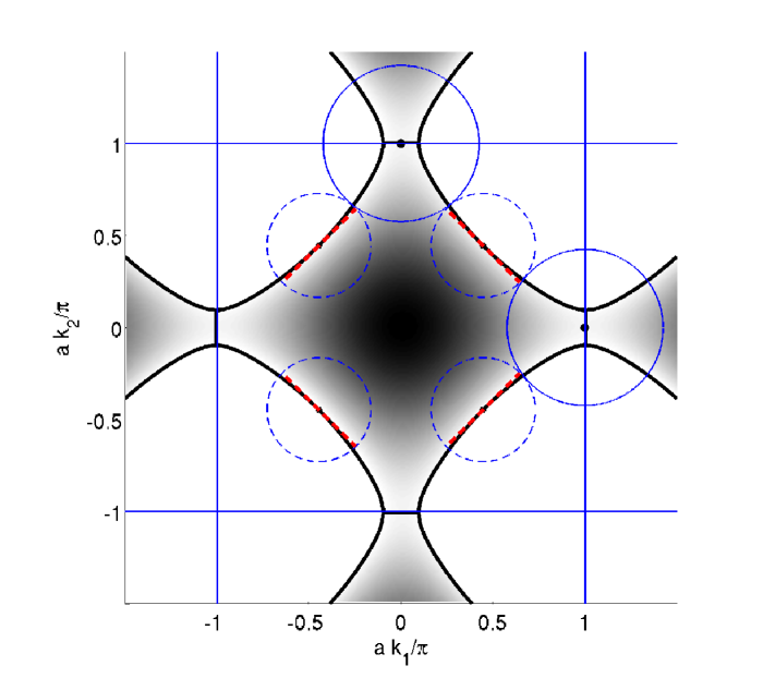
Figure 1: Fermi surface $\epsilon({\bf k})=\mu$ for the tight-binding dispersion relations in (16) for $t^{\prime}/t=-0.2$ and $\mu/t=-0.672$. The full and dashed circles indicate the antinodal respectively nodal regions, as explained in the main text. The dashed lines indicate the Fermi surface arcs we postulate to exist in our approach.

An important parameter determining the physical behavior of HTSC materials is the so-called filling factor $\nu$ defined as the total fermion number divided by the largest possible number of fermions (note that our definition is such that $0\leq\nu\leq 1$). HTSC are typically insulators at half-filling ($\nu=1/2$), and they have a conventional and essentially 2D Fermi surface in the so-called overdoped regime where $\nu$ is significantly different from $1/2$. In the latter regime HTSC behave like conventional metals. Our interest is in the so-called underdoped regime where $\nu$ is close to but different from $1/2$. In this regime HTSC have exotic properties not fully understood. In particular, the Fermi surface in this regime seems to be partially gapped [28]: there still exists a so-called underlying Fermi surface that can be well described by a tight-binding dispersion relation [29] (an example is given in figure 1). The visible part of this Fermi surface consists typically of four line segments called nodal arcs (enclosed by dashed circles in figure 1), and the remaining so-called antinodal parts of the Fermi surface (enclosed by full circles in figure 1) are gapped. The $\nu$-dependence of the size and location of the nodal arcs has been measured for various HTSC materials; see e.g. [29] and references therein.

3.2 Theory

The continuum limit we use to derive the 2D Luttinger model is based on the following hypothesis about interacting fermion systems that can be justified by renormalization group arguments; see e.g. [30], Chapter 12 and 14 or [31], Chapter 4.

• There exists some underlying Fermi surface dominating the low energy physics of the interacting fermion model, and one can modify, ignore or add degrees of freedom far away from this Fermi surface without changing the low energy properties of the model much.

As a motivation we first recall the well-known 1D case [8]. The non-interacting Fermi surface of the 1D $t$-$t^{\prime}$-$V\,$model consists of two points, and according to Hypothesis H1 one can perform a continuum limit that amounts to the following approximations: linearizing the dispersion relation in the vicinity of the Fermi surface points, modifying interactions of degrees of freedom away from these points, and partly removing the short-distance cutoff. One thus obtains a continuum model with two fermion branches, the left- and the right movers, representing the fermion degrees of freedom in vicinity of the two Fermi-surface points. The approximations described above provide crucial simplifications since they lead to a model of interacting fermions that can be mapped exactly to a non-interacting boson model [8].

In 2D the situation is more involved. However, it is still useful to consider a typical non-interacting Fermi surface of the 2D $t$-$t^{\prime}$-$V\,$model. The latter is defined by the following tight-binding dispersion relation

$$\epsilon({\bf k})=-2t[\cos(ak_{1})+\cos(ak_{2})]-4t^{\prime}\cos(ak_{1})\cos(ak_{2})$$ (16)

with ${\bf k}=(k_{1},k_{2})$ the usual momenta in the Brillouin zone $-\pi/a\leq k_{j}<\pi/a$ and the hopping parameters $t>0$ and $t^{\prime}$ ($a>0$ is the lattice constant). As a representative example we plot in figure 1 the Fermi surface $\epsilon({\bf k})=\mu$ for some small negative values of $t^{\prime}/t$ and the Fermi energy $\mu$.

The behavior of the dispersion relation $\epsilon({\bf k})$ is qualitatively different in different regions of the Brillouin zone: since $(\pi/a,0)$ and $(0,\pi/a)$ are saddle points of $\epsilon({\bf k})$, no linear approximation of the dispersion relation exists in the so-called antinodal regions close to these saddle points. However, in the so-called nodal regions close to points ${\bf k}=(Q/a,\pm Q/a)$ and $(-Q/a,\mp Q/a)$ for some parameter $Q\approx\pi/2$, one can approximate by a linear dispersion relation; see (47). (The antinodal and nodal regions are indicated by full respectively dashed circles in figure 1.) This suggests that the fermion degrees of freedom in these different regions play different roles in the interacting model. We thus rewrite the model by introducing field operators $\psi^{({\dagger})}_{r,s}$ labeled by “flavor indices” $r=\pm$ and $s=0,\pm$ that represent the fermion degrees of freedom in these different regions: $r=\pm$ and $s=\pm$ correspond to the regions close to the nodal points $(rQ/a,srQ/a)$, and $r=\pm$ and $s=0$ correspond to the regions close to the antinodal points $(\pi/a,0)$ and $(0,\pi/a)$, respectively. Before we can use H1 above to modify the model we need another hypothesis that is partly motivated by experiments on HTSC mentioned in Section 3.1:

• The underlying Fermi surface contains nodal arcs that can be well approximated by straight line segments.

To be more specific, we assume that the Fermi surface contains four points $(Q/a,\pm Q/a)$ and $(-Q/a,\mp Q/a)$ for some parameter $Q\approx\pi/2$, and that close to each of these points we can approximate the exact dispersion relation by the linearized one. As will be seen, this corresponds to a Fermi surface containing four straight line segments as indicated by the dashed lines in figure 1. We introduce a parameter $\kappa$ determining the size of the regions where we use the linearized dispersion relations and such that the length of these line segments is $(1-\kappa)\sqrt{2}\pi/a$. We emphasize that we do not make any assumption about the underlying Fermi surface in the antinodal region, and whether the antinodal regions are gapped or not depends on parameters and can be determined by computations [11].

Our approximations leading to the 2D Luttinger model are similar to the ones in 1D mentioned above. They are (essentially) justified by Hypotheses H1 and H2 above. Similarly as in 1D, due to their linear dispersion relation, the interacting nodal fermions can be mapped exactly to non-interacting bosons.

4 Definitions and notation

We write “$\stackrel{{\scriptstyle\mbox{{\tiny def}}}}{{=}}$” to emphasize that an equality is a definition. We write a vector ${\bf k}\in{\mathbb{R}}^{2}$ in components either as ${\bf k}=(k_{1},k_{2})$, $k_{j}\in{\mathbb{R}}$, or as ${\bf k}=k_{+}{\bf e}_{+}+k_{-}{\bf e}_{-}$ with

$$k_{\pm}\stackrel{{\scriptstyle\mbox{{\tiny def}}}}{{=}}(k_{1}\pm k_{2})/\sqrt{2},\quad{\bf e}_{\pm}\stackrel{{\scriptstyle\mbox{{\tiny def}}}}{{=}}(1,\pm 1)/\sqrt{2},$$

and $|{\bf k}|\stackrel{{\scriptstyle\mbox{{\tiny def}}}}{{=}}\sqrt{k_{+}^{2}+k_{-}^{2}}$. We use symbols ${\bf x},{\bf y}$ for fermion positions, ${\bf k},{\bf k}^{\prime}$ for fermion momenta, and ${\bf p}$ for differences of fermion momenta.

We write “$k_{\pm}<c$” short for “$k_{+}<c$ and $k_{-}<c$” etc., and “$k_{\pm}\not<c$” is short for “$k_{+}\not<c$ or $k_{-}\not<c$ (or both)” etc.

4.1 2D $t$-$t^{\prime}$-$V\,$model

We consider a diagonal square lattice $\Lambda$ with lattice constant $a>0$ and $(L/a)^{2}\gg 1$ lattice sites: The lattice sites are ${\bf x}=(x_{1},x_{2})=(an_{1},an_{2})$ with integers $n_{j}$ such that $-L/2\leq x_{\pm}<L/2$, and we assume that $L/(2\sqrt{2}a)\in{\mathbb{N}}$. The momenta we use are therefore restricted to be in the following sets,

$$\begin{split}\Lambda^{*}\stackrel{{\scriptstyle\mbox{{\tiny def}}}}{{=}}&\left\{{\bf k}\in{\mathbb{R}}^{2}:\;k_{\pm}\in\mbox{$\frac{2\pi}{L}$}({\mathbb{Z}}+\mbox{$\frac{1}{2}$})\right\}\\ \tilde{\Lambda}^{*}\stackrel{{\scriptstyle\mbox{{\tiny def}}}}{{=}}&\left\{{\bf p}\in{\mathbb{R}}^{2}:\;p_{\pm}\in\mbox{$\frac{2\pi}{L}$}{\mathbb{Z}}\right\}\end{split}$$ (17)

(we use antiperiodic boundary conditions for the fermions). The Brillouin zone (lattice Fourier space) for the fermions is

$$\mathrm{BZ}\stackrel{{\scriptstyle\mbox{{\tiny def}}}}{{=}}\left\{{\bf k}\in\Lambda^{*}:\;-\frac{\pi}{a}\leq k_{j}<\frac{\pi}{a},\quad j=1,2\right\}.$$ (18)

The 2D $t$-$t^{\prime}$-$V\,$model is defined on a Fock space with fermion creation- and annihilation operators $\psi^{({\dagger})}({\bf x})$ labeled by lattice vectors ${\bf x}$ and satisfying the usual canonical anticommutator relations. We denote as $|0\rangle$ the normalized vacuum state annihilated by all $\psi({\bf x})$, and our normalization is such that $\{\psi({\bf x}),\psi^{\dagger}({\bf y})\}=\delta_{{\bf x},{\bf y}}/a^{2}$. The Hamiltonian of this model is

$$H_{tt^{\prime}V}=H_{0}+H^{\prime}$$ (19)

with the free part

$$H_{0}=\sum_{{\bf x},{\bf y}\in\Lambda}a^{4}[-T({\bf x}-{\bf y})-\mu\delta_{{\bf x},{\bf y}}/a^{2}]\psi^{\dagger}({\bf x})\psi({\bf y})$$ (20)

and the hopping matrix $T({\bf x}-{\bf y})$ equal to $t/a^{2}>0$ for nearest neighbor sites (i.e. if $|{\bf x}-{\bf y}|=a$), $t^{\prime}/a^{2}$ for next-nearest neighbor sites (i.e. if $|{\bf x}-{\bf y}|=\sqrt{2}a$), and zero otherwise; $\mu\in{\mathbb{R}}$ is the chemical potential. The interaction part is

$$H^{\prime}=\sum_{{\bf x},{\bf y}\in\Lambda}a^{4}u({\bf x}-{\bf y})\psi^{\dagger}({\bf x})\psi({\bf x})\psi^{\dagger}({\bf y})\psi({\bf y})$$ (21)

with $u({\bf x}-{\bf y})=V/4>0$ for nearest neighbor sites ${\bf x}$, ${\bf y}$ and zero otherwise. Note that our scaling with $a$ is such that $t$, $t^{\prime}$, $V$ and $\mu$ all have the dimensions of an energy. We assume that $|2t^{\prime}/t|<1$ (otherwise the qualitative features of the dispersion relation are different from what we assume in Section 5 and our treatment does not apply).

The average number of fermions per site is the filling factor (or filling) defined as follows,

$$\nu\stackrel{{\scriptstyle\mbox{{\tiny def}}}}{{=}}\left(\mbox{$\frac{a}{L}$}\right)^{2}\langle N\rangle,\quad N\stackrel{{\scriptstyle\mbox{{\tiny def}}}}{{=}}\sum_{{\bf x}\in\Lambda}a^{2}\psi^{\dagger}({\bf x})\psi({\bf x})$$ (22)

where $\langle\cdot\rangle$ is the ground (or thermal) state expectation value and $N$ the fermion number operator. Thus $0\leq\nu\leq 1$, and half-filling corresponds to $\nu=1/2$. We sometimes refer to $\nu-1/2$ as doping.

We recall that the model is invariant under the particle-hole transformation $\psi({\bf x})\leftrightarrow(-1)^{(x_{1}+x_{2})/a}\psi^{\dagger}({\bf x})$ equivalent to the following change of parameters

$$(t,t^{\prime},\nu,\mu,V)\to(t,-t^{\prime},1-\nu,2V-\mu,V).$$ (23)

The model is also invariant under the following (discrete) rotation and parity transformations

$$\mathcal{R}:\;{\bf x}=(x_{1},x_{2})\to(-x_{2},x_{1}),\quad\mathcal{P}:\;{\bf x}\to-{\bf x}.$$ (24)

Our conventions for Fourier transformation are as follows,

$$\hat{\psi}({\bf k})=\frac{1}{2\pi}\sum_{{\bf x}\in\Lambda}a^{2}\psi({\bf x})\,\mathrm{e}^{-\mathrm{i}{\bf k}\cdot{\bf x}}$$

with ${\bf k}\in\mathrm{BZ}$. This allows us to write

$$H_{0}=\sum_{{\bf k}\in\mathrm{BZ}}(\mbox{$\frac{2\pi}{L}$})^{2}[\epsilon({\bf k})-\mu]\hat{\psi}^{\dagger}({\bf k})\hat{\psi}({\bf k})$$ (25)

with the dispersion relation in (16). The interaction part in Fourier space is

$$H^{\prime}=\sum_{{\bf k}_{j}\in\mathrm{BZ}}\left(\mbox{$\frac{2\pi}{L}$}\right)^{8}\hat{v}({\bf k}_{1},{\bf k}_{2},{\bf k}_{2},{\bf k}_{4})\,\hat{\psi}^{\dagger}({\bf k}_{1})\hat{\psi}({\bf k}_{2})\hat{\psi}^{\dagger}({\bf k}_{3})\hat{\psi}({\bf k}_{4})$$ (26)

with

$$\hat{v}({\bf k}_{1},{\bf k}_{2},{\bf k}_{3},{\bf k}_{4})=\hat{u}({\bf k}_{1}-{\bf k}_{2})\sum_{{\bf n}\in{\mathbb{Z}}^{2}}\left(\mbox{$\frac{L}{2\pi}$}\right)^{2}\delta_{{\bf k}_{1}-{\bf k}_{2}+{\bf k}_{3}-{\bf k}_{4},2\pi{\bf n}/a}$$ (27)

and

$$\hat{u}({\bf p})=\frac{a^{2}V}{8\pi^{2}}[\cos(ap_{1})+\cos(ap_{2})].$$ (28)

The physical interpretation of our interaction is that it contains all possible scattering terms ${\bf k}_{4}\to{\bf k}_{3}$ and ${\bf k}_{2}\to{\bf k}_{1}$ weighted by a factor $\hat{u}({\bf k}_{1}-{\bf k}_{2})$ and otherwise restricted only by overall momentum conservation up to umklapp processes.

We also use fermion density operators

$$\rho({\bf x})\stackrel{{\scriptstyle\mbox{{\tiny def}}}}{{=}}\psi^{\dagger}({\bf x})\psi({\bf x})$$

with the following conventions for Fourier transformation

$$\hat{\rho}({\bf p})=\sum_{{\bf x}\in\Lambda}a^{2}\rho({\bf x})\,\mathrm{e}^{-\mathrm{i}{\bf p}\cdot{\bf x}}=\sum_{{\bf k}_{1},{\bf k}_{2}\in\mathrm{BZ}}\hat{\psi}^{\dagger}({\bf k}_{1})\hat{\psi}({\bf k}_{2})\sum_{{\bf n}\in{\mathbb{Z}}^{2}}\delta_{{\bf k}_{1}+{\bf p},{\bf k}_{2}+2\pi{\bf n}/a}$$

for ${\bf p}\in\tilde{\Lambda}^{*}$ such that $|p_{\pm}|\leq\pi/a$. This allows us to write

$$H^{\prime}=\sum_{{\bf x},{\bf y}}a^{4}u({\bf x}-{\bf y})\rho({\bf x})\rho({\bf y})=\sum_{{\bf p}}\mbox{$(\frac{1}{L})^{2}$}\hat{u}({\bf p})\hat{\rho}(-{\bf p})\hat{\rho}({\bf p}).$$

Our conventions for density operators of the 2D Luttinger model are similar.

Remark: Note that our normalizations are such that the naive continuum limit $a\to 0$ makes sense, in particular $\delta_{{\bf x},{\bf y}}/a^{2}\to\delta^{2}({\bf x}-{\bf y})$ (Dirac delta) and $\sum_{{\bf x}}a^{2}\to\int d^{2}x$ (Riemann sum). This limit corresponds to the one discussed in Section 7, remark 4. However, we are mainly interested in the continuum limit where $\nu$ is fixed and close to $1/2$, and this limit is more delicate. Note also that our formulas have a well-defined limit $L\to\infty$, in particular, $\{\hat{\psi}({\bf k}),\hat{\psi}^{\dagger}({\bf k}^{\prime})\}=[L/(2\pi)]^{2}\delta_{{\bf k},{\bf k}^{\prime}}\to\delta^{2}({\bf k}-{\bf k}^{\prime})$ and $\sum_{{\bf k}}(2\pi/L)^{2}\to\int d^{2}k$.

4.2 2D Luttinger model

The formal definition of the 2D Luttinger model in Section 2 can be made mathematically precise as follows.

The 2D Luttinger model is an effective model for the 2D $t$-$t^{\prime}$-$V\,$model depending on two more parameters $\kappa$ and $Q$ in the ranges given in (5) and such that

$$\kappa\in\frac{2\sqrt{2}a}{L}({\mathbb{N}}+\mbox{$\frac{1}{2}$}),\quad Q\in\frac{\sqrt{2}\pi a}{L}{\mathbb{N}}$$ (29)

(it would be easy to drop the restrictions in (29), but they simplify some formulas below, and they become irrelevant for $L/a\gg 1$).

We introduce fermion operators $\hat{\psi}^{({\dagger})}_{r,s}({\bf k})$ labeled by two indices $s=0,\pm$ and $r=\pm$ and by momenta ${\bf k}$ in different Fourier spaces $\Lambda^{*}_{s}$ as follows,

$$\begin{split}\Lambda^{*}_{0}=&\left\{{\bf k}\in\Lambda^{*}:\;|k_{\pm}+\mbox{$\frac{\pi}{L}$}|<\frac{\kappa\pi}{\sqrt{2}a}\right\}\\ \Lambda^{*}_{s=\pm}=&\left\{{\bf k}\in\Lambda^{*}:\;|k_{-s}+\mbox{$\frac{\pi}{L}$}|<\frac{(1-\kappa)\pi}{\sqrt{2}a}\right\}.\end{split}$$ (30)

Note that there are infinitely many nodal (i.e. $s=\pm$) fermion degrees of freedom (since there is no restriction in $\Lambda^{*}_{s=\pm}$ on $k_{s}$), but only finitely many antinodal (i.e. $s=0$) ones. These fermion operators obey the usual canonical anticommutator relations normalized such that

$$\{\hat{\psi}^{\phantom{{\dagger}}}_{r,s}({\bf k}),\hat{\psi}^{\dagger}_{r^{\prime},s^{\prime}}({\bf k}^{\prime})\}=\delta_{r,r^{\prime}}\delta_{s,s^{\prime}}\delta_{{\bf k},{\bf k}^{\prime}}(\mbox{$\frac{2\pi}{L}$})^{2},$$ (31)

and they are defined on a Fock space with a non-trivial vacuum $\Omega$ (“Dirac sea”) characterized by the following conditions,

$$\hat{\psi}^{\phantom{{\dagger}}}_{r,s=\pm}({\bf k})\Omega=\hat{\psi}^{\dagger}_{r,s=\pm}(-{\bf k})\Omega=0\quad\forall{\bf k}\,\mbox{ such that }\,rk_{s}>0$$ (32)

and $\langle\Omega,\Omega\rangle=1$, with $\langle\cdot,\cdot\rangle$ the Fock space inner product. For the antinodal fermions we only assume that antinodal filling is the same for $r=+$ and $r=-$, i.e.

$$\nu_{a}\stackrel{{\scriptstyle\mbox{{\tiny def}}}}{{=}}\frac{2}{(\kappa L)^{2}}\sum_{{\bf k}\in\Lambda^{*}_{0}}(\mbox{$\frac{2\pi}{L}$})^{2}\langle\Omega,\hat{\psi}^{\dagger}_{r,0}({\bf k})\hat{\psi}^{\phantom{{\dagger}}}_{r,0}({\bf k})\Omega\rangle$$ (33)

is independent of $r=\pm$. The latter assumption could be easily dropped, but it simplifies some formulas, and it can be checked at the end of our computations. Note that $0\leq\nu_{a}\leq 1$, i.e. $\nu_{a}$ defined in (33) is the filling factor for the antinodal fermions. It is not a free parameter but can be computed self-consistently [11]. We denote by colons normal ordering with respect to $\Omega$ as usual,

$$:\!A\!:\;\stackrel{{\scriptstyle\mbox{{\tiny def}}}}{{=}}A-\langle\Omega,A\Omega\rangle$$ (34)

for fermion bilinear operators $A=\hat{\psi}^{\dagger}_{r,s}({\bf k})\hat{\psi}^{\phantom{{\dagger}}}_{r,s}({\bf k}^{\prime})$ etc. (boson operators are normal ordered in the same way in Section 6). We also introduce the cutoff functions

$$\chi_{s=\pm}({\bf p})=\begin{cases}1&\mbox{ if }\;|p_{s}|\leq\frac{\kappa\pi}{\sqrt{2}a}\;\mbox{ and }\;|p_{-s}|\leq\frac{(1-\kappa)\pi}{\sqrt{2}a}\\ 0&\mbox{ otherwise.}\end{cases}$$ (35)

The 2D Luttinger model is defined by the Hamiltonian $H=H_{n}+H_{a}+H_{na}$ with

$$\begin{split}H_{n}=&\sum_{s=\pm}\sum_{{\bf k}\in\Lambda^{*}_{s}}(\mbox{$\frac{2\pi}{L}$})^{2}\sum_{r=\pm}rv_{F}k_{s}:\!\hat{\psi}^{\dagger}_{r,s}({\bf k})\hat{\psi}^{\phantom{{\dagger}}}_{r,s}({\bf k})\!:\\ &+2\sum_{{\bf p}\in\tilde{\Lambda}^{*}}\mbox{$(\frac{1}{L})^{2}$}\Bigl{(}g_{1}\sum_{s=\pm}\chi_{s}({\bf p})\hat{J}_{+,s}(-{\bf p})\hat{J}_{-,s}({\bf p})+g_{2}\sum_{r,r^{\prime}=\pm}\chi_{+}({\bf p})\chi_{-}({\bf p})\hat{J}_{r,+}(-{\bf p})\hat{J}_{r^{\prime},-}({\bf p})\Bigr{)}\end{split}$$ (36)

the nodal part,

$$\begin{split}H_{a}=&\sum_{{\bf k}\Lambda^{*}_{0}}(\mbox{$\frac{2\pi}{L}$})^{2}\sum_{r=\pm}[-rc_{F}k_{+}k_{-}-c_{F}^{\prime}(k_{+}^{2}+k_{-}^{2})-\mu_{0}]:\!\hat{\psi}^{\dagger}_{r,0}({\bf k})\hat{\psi}^{\phantom{{\dagger}}}_{r,0}({\bf k})\!:\\ &+2\sum_{{\bf p}\in\tilde{\Lambda}^{*}}\mbox{$(\frac{1}{L})^{2}$}\,g_{3}\hat{J}_{+,0}(-{\bf p})\hat{J}_{-,0}({\bf p})\end{split}$$ (37)

the antinodal part, and

$$H_{na}=\sum_{{\bf p}\in\tilde{\Lambda}^{*}}\mbox{$(\frac{1}{L})^{2}$}\,g_{4}\sum_{r,r^{\prime}}\hat{J}_{r,0}(-{\bf p})\sum_{s=\pm}\chi_{s}({\bf p})\hat{J}_{r^{\prime},s}({\bf p})$$ (38)

the mixed part. The interactions involve the following Fourier transformed and normal ordered fermion densities,

$$\begin{split}\hat{J}_{r,0}({\bf p})=&\sum_{{\bf k}\in\Lambda^{*}_{0}}(\mbox{$\frac{2\pi}{L}$})^{2}:\!\hat{\psi}^{\dagger}_{r,0}({\bf k}-{\bf p})\hat{\psi}^{\phantom{{\dagger}}}_{r,0}({\bf k})\!:\\ \hat{J}_{r,s=\pm}({\bf p})=&\sum_{{\bf k}\in\Lambda^{*}_{s}}(\mbox{$\frac{2\pi}{L}$})^{2}\sum_{n\in{\mathbb{Z}}}:\!\hat{\psi}^{\dagger}_{r,s}({\bf k}-{\bf p})\hat{\psi}^{\phantom{{\dagger}}}_{r,s}({\bf k}+\sqrt{2}(1-\kappa)\pi n{\bf e}_{-s}/a)\!:.\end{split}$$ (39)

The model parameters are given in (6)–(9). As mentioned, the 2D Luttinger model is well-defined if $\gamma$ in (14) satisfies the condition $\gamma<1$, and we always assume this is the case.

As discussed in more detail below, normal ordering is essential to make the terms involving nodal fermions well-defined, but for the antinodal fermions it only amounts to subtracting finite constants. Note that $\hat{J}_{r,0}({\bf p})$ is non-zero only for $|p_{\pm}|\leq\sqrt{2}\pi\kappa/a$, and $\hat{J}_{r,s=\pm}({\bf p})$ is defined for ${\bf p}$ in

$$\mathrm{C}_{s=\pm}=\left\{{\bf p}\in\tilde{\Lambda}^{*}\,:\,|p_{-s}|\leq\frac{\pi(1-\kappa)}{\sqrt{2}a}\right\}.$$ (40)

The relation between the precise definition of the 2D Luttinger model here and the formal one in Section 2 is spelled out in Section 5.5.

5 Derivation of the 2D Luttinger model

5.1 Eight flavor model

We divide our Brillouin zone in eight non-overlapping regions as indicated in figure 2. For that we define eight vectors ${\bf Q}_{r,s}$ with $r=\pm$ and $s=0,\pm,2$ as follows

$$\begin{split}&{\bf Q}_{+,0}=(\pi/a,0),\quad{\bf Q}_{-,0}=(0,\pi/a)\\ &{\bf Q}_{r,s}=(rQ/a,rsQ/a)\;\mbox{ for }\;r=\pm,s=\pm\\ &{\bf Q}_{-,2}=(0,0),\quad{\bf Q}_{+,2}=(\pi/a,\pi/a)\end{split}$$ (41)

for some $Q\approx\pi/2$ obeying the second condition in (5). We also introduce eight corresponding rectangular regions $\Lambda^{*}_{r,s}$ so that every vector in $\mathrm{BZ}$ can be written uniquely as ${\bf Q}_{r,s}+{\bf k}+2\pi{\bf n}/a$ for some $r\in\{+,-\}$, $s\in\{0,\pm,2\}$, ${\bf k}\in\Lambda^{*}_{r,s}$, and ${\bf n}\in{\mathbb{Z}}^{2}$ (the umklapp term $2\pi{\bf n}/a$ is sometimes needed to translate to the region $-\pi/a\leq k_{j}<\pi/a$). Mathematically these regions can be defined as follows

$$\begin{split}\Lambda^{*}_{r,0}=&\left\{{\bf k}\in\mathrm{BZ}:\;|k_{\pm}+\mbox{$\frac{\pi}{L}$}|<\frac{\kappa\pi}{\sqrt{2}a}\right\}\\ \Lambda^{*}_{r,s=\pm}=&\left\{{\bf k}\in\mathrm{BZ}:\;\left|k_{s}+\mbox{$\frac{\pi}{L}$}+r\frac{(2Q-\pi)}{\sqrt{2}a}\right|<\frac{\kappa\pi}{\sqrt{2}a},\quad\left|k_{-s}+\mbox{$\frac{\pi}{L}$}\right|<\frac{(1-\kappa)\pi}{\sqrt{2}a}\right\}\\ \Lambda^{*}_{r,2}=&\left\{{\bf k}\in\mathrm{BZ}:\;\left|k_{\pm}+\mbox{$\frac{\pi}{L}$}\right|<\frac{(1-\kappa)\pi}{\sqrt{2}a}\right\}\end{split}$$ (42)

for some parameter $\kappa$ satisfying the first condition in (5) (see figure 2). Thus our division of the Brillouin zone depends on two parameters $Q$ and $\kappa$ where the former specifies the locations and the latter the size of the Fermi surface arcs. It is easy to see that, for geometric reasons, $\kappa$ and $Q$ are restricted as in (5). Note that $\Lambda^{*}_{r,0}$ is the same for $r=+$ and $r=-$ and equal to $\Lambda^{*}_{0}$ in (30).

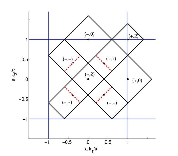
Figure 2: Division of the Brillouin zone $\mathrm{BZ}$ in eight regions ${\bf Q}_{r,s}+\Lambda^{*}_{r,s}$ marked as $(r,s)$ for $r=\pm$, $s=0,\pm,2$; see (41) and (42). The eight dots mark the points ${\bf Q}_{r,s}$, and the parameters are $Q=0.45\pi$ and $\kappa=0.8$. Note that $k_{1,2}$ can be shifted by integer multiples of $2\pi/a$ so that the union of these regions cover the $\mathrm{BZ}$ exactly once.

We define

$$\hat{\psi}_{r,s}({\bf k})\stackrel{{\scriptstyle\mbox{{\tiny def}}}}{{=}}\hat{\psi}({\bf Q}_{r,s}+{\bf k}+2\pi{\bf n}/a)\quad\forall{\bf k}\in\Lambda^{*}_{r,s}$$

with ${\bf n}\in{\mathbb{Z}}^{2}$ such that ${\bf Q}_{r,s}+{\bf k}+2\pi{\bf n}/a\in\mathrm{BZ}$. This allows us to rewrite the free- and interaction parts of our Hamiltonian in (25) and (26) as follows,

$$H_{0}=\sum_{r,s}\sum_{{\bf k}\in\Lambda^{*}_{r,s}}(\mbox{$\frac{2\pi}{L}$})^{2}[\epsilon({\bf Q}_{r,s}+{\bf k})-\mu]\hat{\psi}^{\dagger}_{r,s}({\bf k})\hat{\psi}^{\phantom{{\dagger}}}_{r,s}({\bf k})$$

and

$$H^{\prime}=\sum_{r_{j},s_{j}}\sum_{{\bf k}_{j}\in\Lambda^{*}_{r_{j},s_{j}}}\left(\mbox{$\frac{2\pi}{L}$}\right)^{8}\hat{v}(K_{1},K_{2},K_{3},K_{4})\,\hat{\psi}^{\dagger}_{r_{1},s_{1}}({\bf k}_{1})\hat{\psi}^{\phantom{{\dagger}}}_{r_{2},s_{2}}({\bf k}_{2})\hat{\psi}^{\dagger}_{r_{3},s_{3}}({\bf k}_{3})\hat{\psi}^{\phantom{{\dagger}}}_{r_{4},s_{4}}({\bf k}_{4})$$

where $K_{j}$ is short for $({\bf k}_{j},r_{j},s_{j})$ and

$$\begin{split}\hat{v}(K_{1},K_{2},K_{3},K_{4})=&\hat{u}({\bf Q}_{r_{1},s_{1}}-{\bf Q}_{r_{2},s_{2}}+{\bf k}_{1}-{\bf k}_{2})\sum_{{\bf n}\in{\mathbb{Z}}^{2}}\left(\mbox{$\frac{L}{2\pi}$}\right)^{2}\\ &\times\delta_{{\bf Q}_{r_{1},s_{1}}-{\bf Q}_{r_{2},s_{2}}+{\bf Q}_{r_{3},s_{3}}-{\bf Q}_{r_{4},s_{4}}+{\bf k}_{1}-{\bf k}_{2}+{\bf k}_{3}-{\bf k}_{4},2\pi/a{\bf n}}.\end{split}$$ (43)

The fermion number operator can now be written as

$$N=\sum_{{\bf k}\in\mathrm{BZ}}(\mbox{$\frac{2\pi}{L}$})^{2}\hat{\psi}^{\dagger}({\bf k})\hat{\psi}({\bf k})=\sum_{r,s}N_{r,s},\quad N_{r,s}=\sum_{{\bf k}\in\Lambda^{*}_{r,s}}(\mbox{$\frac{2\pi}{L}$})^{2}\hat{\psi}^{\dagger}_{r,s}({\bf k})\hat{\psi}^{\phantom{{\dagger}}}_{r,s}({\bf k})$$ (44)

where $N_{r,s}$ is the number operator for the $(r,s)$ fermions.

Note that, up to now, we only rewrote the lattice Hamiltonian without any approximation. However, we now can interpret it as model of eight different flavors of fermions distinguished by the labels $s$ and $r$. The degrees of freedom with the flavor index $s=0$, $r=\pm$ are what we call antinodal fermions, and the ones with $s=\pm$, $r=\pm$ are the nodal fermions. We call the degrees of freedom with $s=2$ for $r=-$ and $r=+$ the in- and the out fermions, respectively.

We have introduced two parameters $Q$ and $\kappa$ for generality, and the effective model we derive below depends on them. In principle these parameters can be determined from filling and by minimizing the total energy, but for now we leave them arbitrary. We note that the choice $\kappa=1/2$ and $Q=\pi/2$ is special since then all the “small” Fourier space regions $\Lambda^{*}_{r,s}$ are identical and equal to the Brillouin zone of a “large” lattice with sites ${\bf X}=n_{1}(1,1)a+n_{2}(-1,1)a$, $n_{j}$ integers, which contains eight sites of the original lattice per elementary cell. However, it is important to note that our eight flavor model is not local on this “large” lattice.

Our fermion flavors $(r,s)$ can be naturally divided into four different classes with different physical behavior: (i) $(+,0)$ and $(-,0)$ (antinodal fermions), (ii) $(+,+)$, $(-,+)$, $(+,-)$ and $(-,-)$ (nodal fermions), (iii) $(-,2)$ (in-fermions), and (iv) $(+,2)$ (out-fermions). It is interesting to note that this division of fermions in four classes is also implied by symmetry considerations: The (discrete) rotation and parity transformations in (24) mix our fermion flavors $(r,s)$ as follows,

$$\begin{split}\mathcal{R}:&\;(r,0)\to(-r,0),\quad(r,\pm)\to(\pm r,\mp),\quad(r,2)\to(r,2)\\ \mathcal{P}:&\;(r,0)\to(r,0),\quad(r,\pm)\to(-r,\pm),\quad(r,2)\to(r,2)\end{split}$$ (45)

for $r=\pm$. Thus the four fermion classes above transform under different irreducible representations of the group generated by ${\cal R}$ and ${\cal P}$.

5.2 Partial continuum limit I

We indent to modify the short-distance details of the eight flavor model such that it becomes amenable to exact, non-perturbative computations. For that we follow a strategy which has been successfully used in 1D: We assume that there is some underlying Fermi surface dominating the low energy physics, and we can modify, ignore or add degrees of freedom far away from this Fermi surface (in the latter two cases we need to correct the definition of doping, of course); see Section 3.2 for physical arguments motivating this strategy.

We expand the dispersion relations of the different fermion flavors $(r,s)$ in Taylor series in $k_{\pm}$, and we denote the lowest order non-trivial terms as $\varepsilon_{r,s}$,

$$\epsilon({\bf Q}_{r,s}+{\bf k})=\epsilon({\bf Q}_{r,s})+\varepsilon_{r,s}({\bf k})+\ldots$$

with the dots indicating higher order terms. We find

$$\epsilon({\bf Q}_{r,0})=4t^{\prime},\quad\epsilon({\bf Q}_{r,\pm})=-4[t\cos(Q)+t^{\prime}\cos^{2}(Q)],\quad\epsilon({\bf Q}_{r,2})=4(rt-t^{\prime})$$ (46)

and

$$\begin{split}\varepsilon_{r,0}({\bf k})&=-rc_{F}k_{+}k_{-}-c_{F}^{\prime}(k_{+}^{2}+k_{-}^{2}),\\ \varepsilon_{r,\pm}({\bf k})&=rv_{F}k_{\pm},\\ \varepsilon_{r,2}({\bf k})&=(-\mbox{$\frac{1}{2}$}rc_{F}+c_{F}^{\prime})(k_{+}^{2}+k_{-}^{2})\end{split}$$ (47)

with the constants in (6). We see that the nodal fermions ($s=\pm$) have dispersion relations approximately linear and with a constant Fermi velocity $v_{F}$, but the dispersion relations of the antinodal fermions ($s=0$) are quadratic. The in- and out fermions ($s=2$ with $r=-$ and $r=+$, respectively) have energies far away from the Fermi energy, and we therefore expect that they can be ignored. This will be done below in Approximation A3’.

Our first approximation is in the free part of the Hamiltonian:

• Replace the exact dispersion relations $\epsilon({\bf Q}_{r,s}+{\bf k})$ in $H_{0}$ by the truncated Taylor series $\epsilon({\bf Q}_{r,s})+\varepsilon_{r,s}({\bf k})$.

This approximation is only essential for the nodal fermions [11], and we use it for the other fermion flavors only for aesthetic consistency.

	$r_{1},s_{1}$	$r_{2},s_{2}$	$r_{3},s_{3}$	$r_{4},s_{4}$	Restrictions
1.	$r,s$	$r,s$	$r^{\prime},s^{\prime}$	$r^{\prime},s^{\prime}$	$(r,s)\neq(r^{\prime},s^{\prime})$, $s,s^{\prime}=0,\pm,2$
2.	$r,s$	$r^{\prime},s^{\prime}$	$r^{\prime},s^{\prime}$	$r,s$	$(r,s)\neq(r^{\prime},s^{\prime})$, $s,s^{\prime}=0,\pm,2$
3.	$r,s$	$r,s$	$r,s$	$r,s$	$s=0,\pm,2$
4.	$r,s$	$-r,s^{\prime}$	$-r,s$	$r,s^{\prime}$	$(s,s^{\prime})=(\pm,\mp),(0,2),(2,0)$
5.	$r,s$	$r,s^{\prime}$	$-r,s$	$-r,s^{\prime}$	$(s,s^{\prime})=(\pm,\mp),(0,2),(2,0)$
6.	$r,s$	$-r,s$	$r,s$	$-r,s$	$s=0,2$
7.	$r,s$	$r^{\prime},s^{\prime}$	$r,s$	$-r^{\prime},s^{\prime}$	$s=0,2$, $s^{\prime}=\pm$
8.	$r,s$	$r^{\prime},s^{\prime}$	$-r,s$	$r^{\prime},s^{\prime}$	$s=\pm$, $s^{\prime}=0,2$
9.	$r,s$	$r^{\prime},s^{\prime}$	$r,s$	$r^{\prime},s^{\prime}$	$s,s^{\prime}=0,2$
10.	$r,s$	$r^{\prime},s^{\prime}$	$-r^{\prime},s^{\prime}$	$-r,s$	$(s,s^{\prime})=(0,2),(2,0)$
11.	$r,s$	$-r,s$	$r^{\prime},s^{\prime}$	$-r^{\prime},s^{\prime}$	$(s,s^{\prime})=(0,2),(2,0)$

Table 1: List of all interactions terms potentially contributing to the effective model derived in Section 5.2; $r,r^{\prime}=\pm$.

Our second approximation is for the interaction part of the Hamiltonian (again this approximation is only essential for terms involving nodal fermions).

• Replace the interaction vertex (43) in $H^{\prime}$ by

  $$\begin{split}\hat{v}(K_{1},K_{2},K_{3},K_{4})=\left(\mbox{$\frac{L}{2\pi}$}\right)^{2}\delta_{{\bf k}_{1}-{\bf k}_{2}+{\bf k}_{3}-{\bf k}_{4},{\boldsymbol{0}}}\,\hat{u}({\bf Q}_{r_{1},s_{1}}-{\bf Q}_{r_{2},s_{2}})\\ \times\sum_{{\bf n}\in{\mathbb{Z}}^{2}}\delta_{{\bf Q}_{r_{1},s_{1}}-{\bf Q}_{r_{2},s_{2}}+{\bf Q}_{r_{3},s_{3}}-{\bf Q}_{r_{4},s_{4}},2\pi/a{\bf n}}.\end{split}$$ (48)

This corresponds to two changes: Firstly, the original interaction vertex in (43) allows all scattering processes such that

$${\bf Q}_{r_{1},s_{1}}-{\bf Q}_{r_{2},s_{2}}+{\bf Q}_{r_{3},s_{3}}-{\bf Q}_{r_{4},s_{4}}+{\bf k}_{1}-{\bf k}_{2}+{\bf k}_{3}-{\bf k}_{4}\in\frac{2\pi}{a}{\mathbb{Z}}^{2}$$

but we now enforce, in addition,

$${\bf Q}_{r_{1},s_{1}}-{\bf Q}_{r_{2},s_{2}}+{\bf Q}_{r_{3},s_{3}}-{\bf Q}_{r_{4},s_{4}}\in\frac{2\pi}{a}{\mathbb{Z}}^{2}.$$ (49)

Secondly, we modify the argument of the weight function $\hat{u}$ in (43) by ignoring the dependence on ${\bf k}_{1}-{\bf k}_{2}$. Since the ${\bf Q}_{r_{j},s_{j}}$ are large and the ${\bf k}_{j}$ (typically) small on the scale of our short-distance cutoff $\pi/a$, we expect that the difference between the original- and our approximate interaction does not change the low energy properties of the model.

We therefore only keep the interaction terms between the fermion flavors for which the condition in (49) is fulfilled. For $Q=\pi/2$ we find 512 such terms, but for $Q\neq\pi/2$ there are only the 196 terms listed in table 1. Below we discuss the corresponding interactions in more detail.

Terms 1 in table 1 are Hartree-like, i.e. they describe scattering processes ${\bf Q}_{r,s}\to{\bf Q}_{r,s}$, ${\bf Q}_{r^{\prime},s^{\prime}}\to{\bf Q}_{r^{\prime},s^{\prime}}$ which preserve fermion flavors. They are given by

$$H^{\prime}_{1}=\sum^{\prime}_{r,s,r^{\prime},s^{\prime}}\sum_{{\bf k}_{j}}(\mbox{$\frac{2\pi}{L}$})^{6}\hat{u}({\boldsymbol{0}})\delta_{{\bf k}_{1}-{\bf k}_{2}+{\bf k}_{3}-{\bf k}_{4},{\boldsymbol{0}}}\,\hat{\psi}^{\dagger}_{r,s}({\bf k}_{1})\hat{\psi}^{\phantom{{\dagger}}}_{r,s}({\bf k}_{2})\hat{\psi}^{\dagger}_{r^{\prime},s^{\prime}}({\bf k}_{3})\hat{\psi}^{\phantom{{\dagger}}}_{r^{\prime},s^{\prime}}({\bf k}_{4})$$

where the prime in the sum indicates that the diagonal terms $(r,s)=(r^{\prime},s^{\prime})$ are excluded (the latter are terms 3 in table 1 and are treated separately). It is useful to introduce the operators

$$\hat{\rho}_{r,s}({\bf p})\stackrel{{\scriptstyle\mbox{{\tiny def}}}}{{=}}\sum_{{\bf k}_{1},{\bf k}_{2}\in\Lambda^{*}_{r,s}}(\mbox{$\frac{2\pi}{L}$})^{2}\hat{\psi}^{\dagger}_{r,s}({\bf k}_{1})\hat{\psi}^{\phantom{{\dagger}}}_{r,s}({\bf k}_{2})\delta_{{\bf k}_{1}+{\bf p},{\bf k}_{2}}$$ (50)

which allow to write the Hartree-like interactions in the following simpler form,

$$H^{\prime}_{1}=\sum^{\prime}_{r,s,r^{\prime},s^{\prime}}\sum_{{\bf p}}(\mbox{$\frac{a}{L}$})^{2}V\hat{\rho}_{r,s}(-{\bf p})\hat{\rho}_{r^{\prime},s^{\prime}}({\bf p})$$ (51)

where we used $(2\pi)^{2}\hat{u}({\boldsymbol{0}})=a^{2}V$. The operators in (50) can be naturally interpreted as Fourier transformed fermion densities.

Terms 2 are Fock-like, i.e. the corresponding scattering processes ${\bf Q}_{r,s}\to{\bf Q}_{r^{\prime},s^{\prime}}$, ${\bf Q}_{r^{\prime},s^{\prime}}\to{\bf Q}_{r,s}$ exchange fermion flavors. They are given by

$$H^{\prime}_{2}=\sum^{\prime}_{r,s,r^{\prime},s^{\prime}}\sum_{{\bf k}_{j}}(\mbox{$\frac{2\pi}{L}$})^{6}\hat{u}({\bf Q}_{r,s}-{\bf Q}_{r^{\prime},s^{\prime}})\delta_{{\bf k}_{1}-{\bf k}_{2}+{\bf k}_{3}-{\bf k}_{4},{\boldsymbol{0}}}\,\hat{\psi}^{\dagger}_{r,s}({\bf k}_{1})\hat{\psi}^{\phantom{{\dagger}}}_{r^{\prime},s^{\prime}}({\bf k}_{2})\hat{\psi}^{\dagger}_{r^{\prime},s^{\prime}}({\bf k}_{3})\hat{\psi}^{\phantom{{\dagger}}}_{r,s}({\bf k}_{4}).$$

Renaming ${\bf k}_{2},{\bf k}_{4}$ to ${\bf k}_{4},{\bf k}_{2}$ and using the anticommutator relations of the fermion field operators we can also write $H^{\prime}_{2}$ in terms of fermion densities,

$$H^{\prime}_{2}=-\sum^{\prime}_{r,s,r^{\prime},s^{\prime}}v_{r,s,r^{\prime},s^{\prime}}\sum_{{\bf p}}(\mbox{$\frac{a}{L}$})^{2}\hat{\rho}_{r,s}(-{\bf p})\hat{\rho}_{r^{\prime},s^{\prime}}({\bf p})+\sum^{\prime}_{r,s,r^{\prime},s^{\prime}}v_{r,s,r^{\prime},s^{\prime}}N_{r,s}f_{r^{\prime},s^{\prime}}$$ (52)

with $N_{r,s}=\hat{\rho}_{r,s}({\boldsymbol{0}})$ equal to the number operators in (44) and the constants

$$v_{r,s,r^{\prime},s^{\prime}}\stackrel{{\scriptstyle\mbox{{\tiny def}}}}{{=}}(2\pi)^{2}\hat{u}({\bf Q}_{r,s}-{\bf Q}_{r^{\prime},s^{\prime}})/a^{2}=v_{r^{\prime},s^{\prime},r,s}$$

and $f_{r,s}\stackrel{{\scriptstyle\mbox{{\tiny def}}}}{{=}}\sum_{{\bf k}\in\Lambda^{*}_{r,s}}(a/L)^{2}$. By simple computations we find

$$\begin{split}v_{+,0,-,0}&=v_{+,2,-,2}=-V,\quad v_{+,\pm,-,\pm}=V\cos(2Q)\\ v_{r,0,r^{\prime},\pm}&=v_{r,0,r^{\prime},2}=0,\quad v_{r,\pm,r^{\prime},\mp}=\mbox{$\frac{1}{2}$}V[1+\cos(2Q)]\\ v_{r,\pm,-,2}&=V\cos(Q),\quad v_{r,\pm,+,2}=-V\cos(Q),\quad v_{r,s,r,s}=V\end{split}$$ (53)

and

$$f_{r,0}=\mbox{$\frac{1}{2}$}\kappa^{2},\quad f_{r,\pm}=\mbox{$\frac{1}{2}$}\kappa(1-\kappa),\quad f_{r,2}=\mbox{$\frac{1}{2}$}(1-\kappa)^{2}$$ (54)

for all $r,r^{\prime}=\pm$. Note that $f_{r,s}$ equals the ratio of the area of $\Lambda^{*}_{r,s}$ to the area of $\mathrm{BZ}$, and $\sum_{r,s}f_{r,s}=1$.

We excluded the diagonal Hartree terms where $(r,s)=(r^{\prime},s^{\prime})$ above since, by simple computations similar to the ones described above, they can be simplified to

$$H^{\prime}_{3}=\sum_{r,s}\sum_{{\bf k},{\bf k}^{\prime}}(\mbox{$\frac{2\pi}{L}$})^{4}\hat{u}({\boldsymbol{0}})\hat{\psi}^{\dagger}_{r,s}({\bf k})\hat{\psi}_{r,s}^{\phantom{{\dagger}}}({\bf k})=\sum_{r,s}VN_{r,s}f_{r,s}$$ (55)

and thus do not contribute to the interactions; see Appendix A for details.

Terms 4 and 5 in table 1 are mixed, i.e. they are Hartree-like in one and Fock-like in the other of the components of the momenta. By straightforward computations one finds that they exactly add up to zero; see Appendix A for details.

Terms 6 are back-scattering terms where the condition in (49) holds true for a non-zero integer vector ${\bf n}$. A simple computations shows that these terms are identical to zero; see Appendix A.

Terms 7–9 are BCS-like, i.e. ${\bf Q}_{r_{1},s_{1}}+{\bf Q}_{r_{3},s_{3}}\in 2\pi{\mathbb{Z}}^{2}/a$ and ${\bf Q}_{r_{2},s_{2}}+{\bf Q}_{r_{4},s_{4}}\in 2\pi{\mathbb{Z}}^{2}/a$ (note that ${\bf Q}_{r,s}+{\bf Q}_{r,s}\in 2\pi{\mathbb{Z}}^{2}/a$ for $s=0,2$ and ${\bf Q}_{r,s}+{\bf Q}_{-r,s}={\boldsymbol{0}}$ for $s=\pm$). Straightforward computations show that all these terms are identically zero; see Appendix A. There are also BCS-like terms $(r_{1},s_{1})=(r,\pm)$, $(r_{2},s_{2})=(-r,\pm)$, $(r_{3},s_{3})=(-r,\pm)$, $(r_{4},s_{4})=(r,\pm)$ which give non-zero contributions, but they are already included in the Fock terms 2 above.

Terms 10 and 11 are back-scattering terms. One can show that the former vanish, and the latter are equal to

$$H^{\prime}_{11}=-V\sum_{{\bf k}_{j}}\sum_{r,r^{\prime}}\left(\mbox{$\frac{2\pi}{L}$}\right)^{4}(\mbox{$\frac{a}{L}$})^{2}\hat{\psi}^{\dagger}_{r,0}({\bf k}_{1})\hat{\psi}^{\phantom{{\dagger}}}_{-r,0}({\bf k}_{2})\hat{\psi}^{\dagger}_{r^{\prime},2}({\bf k}_{3})\hat{\psi}^{\phantom{{\dagger}}}_{-r^{\prime},2}({\bf k}_{4});$$ (56)

see Appendix A.

For $Q=\pi/2$ the equation in (49) has many more solutions. This leads to additional interactions, including, for example,

$$H^{\prime}_{\mathrm{BS}}=V\sum_{{\bf k}_{j}}\sum_{r,r^{\prime}}\sum_{s=\pm}\left(\mbox{$\frac{2\pi}{L}$}\right)^{4}(\mbox{$\frac{a}{L}$})^{2}\hat{\psi}^{\dagger}_{r,0}({\bf k}_{1})\hat{\psi}^{\phantom{{\dagger}}}_{-r,0}({\bf k}_{2})\hat{\psi}^{\dagger}_{r^{\prime},s}({\bf k}_{3})\hat{\psi}^{\phantom{{\dagger}}}_{-r^{\prime},s}({\bf k}_{4}).$$

Nodal back-scattering terms like this, involving nodal fermion operators but which cannot be written in terms of nodal densities $\hat{\rho}_{r,\pm}({\bf p})$, cannot be bosonized in a simple manner. In the following we therefore assume that $Q\neq\pi/2$.

To summarize, we found that, using the Approximations A1 and A2 and assuming $Q\neq\pi/2$, the free- and interaction parts of the 2D $t$-$t^{\prime}$-$V\,$model Hamiltonian are equal to

$$H_{0}=\sum_{r,s}\sum_{{\bf k}}(\mbox{$\frac{2\pi}{L}$})^{2}{[}\epsilon({\bf Q}_{r,s})+\varepsilon_{r,s}({\bf k})-\mu{]}\hat{\psi}^{\dagger}_{r,s}({\bf k})\hat{\psi}^{\phantom{{\dagger}}}_{r,s}({\bf k})$$ (57)

and $H^{\prime}=H^{\prime}_{1}+H^{\prime}_{2}+H^{\prime}_{3}+H^{\prime}_{11}$, i.e.

$$\begin{split}H^{\prime}=\sum^{\prime}_{r,s,r^{\prime},s^{\prime}}(V-v_{r,s,r^{\prime},s^{\prime}})\sum_{{\bf p}}(\mbox{$\frac{a}{L}$})^{2}\hat{\rho}_{r,s}(-{\bf p})\hat{\rho}_{r^{\prime},s^{\prime}}({\bf p})+\sum_{r,s,r^{\prime},s^{\prime}}v_{r,s,r^{\prime},s^{\prime}}N_{r,s}f_{r^{\prime},s^{\prime}}+H^{\prime}_{11}\end{split}$$ (58)

with the dispersion relations in (47) and the constants in (6), (46), (53) and (54). In the following we denote the full Hamiltonian $H_{0}+H^{\prime}$ as $H+H^{\prime}_{11}$ (since $H^{\prime}_{11}$ is not affected by the computations in the next section and will be dropped in Approximation A3’).

Remark: The fact that many of the interaction terms listed in table 1 add up to zero is a consequence of the Pauli exclusion principle and holds true since we use spinless fermions.

5.3 Normal ordering

Up to now we assumed a reference state $|0\rangle$ in the fermion Fock space which is annihilated by all fermion operators $\hat{\psi}({\bf k})$. Before we can partly remove the UV cutoff below (Approximation A4) it is important to introduce another reference state $\Omega$ in which all momentum states ${\bf k}$ inside some Fermi surface are filled. This state can be defined as follows,

$$\Omega\stackrel{{\scriptstyle\mbox{{\tiny def}}}}{{=}}\prod_{{\bf k}}\hat{\psi}^{\dagger}({\bf k})|0\rangle$$

where the product is over the set of all filled momenta ${\bf k}$ specified below. After Approximation A4 below one can only measure physical quantities with respect to this state $\Omega$, i.e., only expectation values of normal ordered operators are finite. We therefore have to determine the effect of normal ordering for various operators of interest to us.

To be more specific, we assume that nodal fermion states ($s=\pm$) are filled up to the Fermi surface arcs described in Section 3.2 (Hypothesis H2) and indicated by dashed lines in figure 1. This is the only assumption we need to make about the Fermi surface since the partial continuum that we perform below only affects the nodal fermions. However, it is also convenient to assume that the antinodal fermions ($s=0$ and $r=\pm$) have some filling $\nu_{a}/2$ which is the same for $r=+$ and $r=-$. We expect that there is an interesting parameter regime with $\nu_{a}=1/2$ [10], but this remains to be shown [11]. It is also convenient to assume that the in- and out fermions ($s=2$ with $r=-$ and $r=+$, respectively) are totally filled and totally empty, respectively. Thus the sets of filled states for the different fermion flavors $r,s$ are as follows,

$$S_{r,\pm}=\left\{{\bf k}\in\Lambda^{*}_{r,\pm}:\;rk_{\pm}<0\right\},\quad S_{-,2}=\Lambda^{*}_{-,2},\quad S_{+,2}=\emptyset$$

and $S_{r,0}$ such that the r.h.s. of (33) is the same for $r=+$ and $r=-$ (as will be seen, we need not be more specific about $S_{r,0}$). This allows us to fully characterize the new reference state as follows,

$$\hat{\psi}^{\dagger}_{r,s}({\bf k})\Omega=0\quad\forall{\bf k}\in S_{r,s},\quad\hat{\psi}^{\phantom{{\dagger}}}_{r,s}({\bf k})\Omega=0\quad\forall{\bf k}\notin S_{r,s}$$

leading to (32) after Approximation A4 below. We compute the contributions $\nu_{r,s}\stackrel{{\scriptstyle\mbox{{\tiny def}}}}{{=}}(a/L)^{2}\langle\Omega,N_{r,s}\Omega\rangle$ of the different fermion flavors to the filling factor in this new reference state and find

$$\nu_{r,0}=\mbox{$\frac{1}{2}$}\nu_{a}\kappa^{2},\quad\nu_{r,\pm}=\mbox{$\frac{1}{4}$}(1-\kappa)\left(\mbox{$\frac{2Q}{\pi}$}-1+\kappa\right),\quad\nu_{-,2}=\mbox{$\frac{1}{2}$}(1-\kappa)^{2},\quad\nu_{+,2}=0$$ (59)

with $\nu_{a}$ in (33), and for the total filling $\sum_{r,s}\nu_{r,s}$ we obtain the result in (9).

We normal order various operators quadratic in the fermion fields as usual; see (34). In particular, the normal ordered fermion number operators are $:\!N_{r,s}\!:\,=N_{r,s}-(L/a)^{2}\nu_{r,s}$. Thus the filling is related to the expectation values of these normal ordered particle number operators as follows,

$$\nu=\mbox{$\frac{1}{2}$}+(1-\kappa)\left(\mbox{$\frac{2Q}{\pi}$}-1\right)+\kappa^{2}(\nu_{a}-\mbox{$\frac{1}{2}$})+\mbox{$(\frac{a}{L})^{2}$}\sum_{r,s}\langle\,:\!N_{r,s}\!:\,\rangle.$$ (60)

To compute the Hamiltonian in its normal ordered form we have to write it in terms of normal ordered fermion densities $\hat{J}_{r,s}({\bf p})\stackrel{{\scriptstyle\mbox{{\tiny def}}}}{{=}}\;:\!\hat{\rho}_{r,s}({\bf p})\!:$. Since normal ordering of these densities is irrelevant unless ${\bf p}=0$ and $\hat{\rho}_{r,s}({\boldsymbol{0}})=N_{r,s}$ we obtain

$$\hat{J}_{r,s}({\bf p})=\hat{\rho}_{r,s}({\bf p})-\delta_{{\bf p},{\boldsymbol{0}}}\,\left(\mbox{$\frac{L}{a}$}\right)^{2}\nu_{r,s}.$$ (61)

Inserting this into the Hamiltonian $H$ obtained at the end of the previous section we get

$$\begin{split}H=&\sum_{r,s}\sum_{{\bf k}\in\Lambda^{*}_{r,s}}(\mbox{$\frac{2\pi}{L}$})^{2}{[}\varepsilon_{r,s}({\bf k})-\mu_{r,s}{]}:\!\hat{\psi}^{\dagger}_{r,s}({\bf k})\hat{\psi}^{\phantom{{\dagger}}}_{r,s}({\bf k})\!:\,\\ &+\sum^{\prime}_{r,s,r^{\prime},s^{\prime}}(V-v_{r,s,r^{\prime},s^{\prime}})\sum_{{\bf p}\in\tilde{\Lambda}^{*}}(\mbox{$\frac{a}{L}$})^{2}\hat{J}_{r,s}(-{\bf p})\hat{J}_{r^{\prime},s^{\prime}}({\bf p})+\mathcal{E}_{0}\end{split}$$ (62)

with the dispersion relations in (47), the parameters

$$\mu_{r,s}=\mu-\epsilon({\bf Q}_{r,s})-2V\sum_{r^{\prime},s^{\prime}}\nu_{r^{\prime},s^{\prime}}-\sum_{r^{\prime},s^{\prime}}v_{r,s,r^{\prime},s^{\prime}}(f_{r^{\prime},s^{\prime}}-2\nu_{r^{\prime},s^{\prime}}),$$ (63)

and the constants in (6), (46), (53), (54) and

$$\mathcal{E}_{0}=\sum_{r=\pm}\sum_{s=0,\pm,2}\sum_{{\bf k}\in\Lambda^{*}_{r,s}}(\mbox{$\frac{2\pi}{L}$})^{2}{[}\epsilon({\bf Q}_{r,s})+\varepsilon_{r,s}({\bf k}){]}\langle\Omega,\hat{\psi}^{\dagger}_{r,s}({\bf k})\hat{\psi}^{\phantom{{\dagger}}}_{r,s}({\bf k})\Omega\rangle+\mathcal{E}_{int}$$ (64)

with

$$\mathcal{E}_{int}=L^{2}\left(V\nu^{2}-\mu\nu+\sum_{r,r^{\prime}=\pm}\sum_{s,s^{\prime}=0,\pm,2}v_{r,s,r^{\prime},s^{\prime}}\nu_{r,s}(f_{r^{\prime},s^{\prime}}-\nu_{r^{\prime},s^{\prime}})\right)$$ (65)

and $\nu$ in (9). The constants $\mu_{r,s}$ correspond to chemical potentials which are different for the different fermion flavors.

The condition that the points ${\bf Q}_{r,\pm}$ are on the Fermi surface is equivalent to $\mu_{r,\pm}=0$, and this fixes the chemical potential $\mu$ and $\mu_{r,s}$ for $r=\pm$ and $s=0,2$. By straightforward computation we find $\mu_{\pm,0}=\mu_{0}$ in (7) and

$$\mu_{\pm,2}=\mp[4t+V(1-\kappa)(1-\kappa+2(\mbox{$\frac{2Q}{\pi}$}-1)\cos(Q))][1\pm\cos(Q)]+4t^{\prime}\sin^{2}(Q).$$ (66)

The particle-hole transformation mentioned in Section 4.1 provides a useful check of our computations above: under this transformation, $\hat{\psi}^{\phantom{{\dagger}}}_{r,s}({\bf k})\leftrightarrow\hat{\psi}^{\dagger}_{-r,s}({\bf k})$, and this is equivalent to the change of parameters in (23) and

$$(Q,\nu_{r,s})\to(\pi-Q,f_{-r,s}-\nu_{-r,s}).$$

Our approximate model above is invariant under this transformation since, in addition, $\mu_{r,s}\to-\mu_{-r,s}$ and $\mathcal{E}_{0}\to\mathcal{E}_{0}$.

Remark: A careful reader might wonder if one could also work with the normal ordered form of the interaction in (21), i.e.

$$H^{\prime}=\sum_{{\bf x},{\bf y}}a^{4}u({\bf x}-{\bf y})\psi^{\dagger}({\bf x})\psi^{\dagger}({\bf y})\psi({\bf y})\psi({\bf x})$$

(this would make the arguments in Section 5.2 somewhat simpler). The answer is “no” since Approximation A2 would spoil particle-hole transformation symmetry then.

5.4 Partial continuum limit II

We assume that the parameters are such that

$$\mu_{-,2}\ll 0,\quad\mu_{+,2}\gg 0$$ (67)

on an energy scale of order $t/5$ or so. This gives some restrictions on the allowed parameter values that are important to check. If these conditions are fulfilled the in- and out fermions ($s=2$ with $r=-$ and $r=+$, respectively) have energies sufficiently far below and far above the Fermi energy, respectively, that the following approximation is expected to be appropriate.

• Drop all terms in the total Hamiltonian involving in- or out fermions.

In particular we drop the interaction term $H^{\prime}_{11}$. Thus the total Hamiltonian is as in (62), but from now on sums over $r,s$ are restricted to $r=\pm$ and $s=0,\pm$ unless stated otherwise. We thus obtain a model involving only nodal and antinodal fermions.

We recall that $\hat{J}_{r,s}({\bf p})$ is proportional to the sum of all terms $:\!\hat{\psi}^{\dagger}_{r,s}({\bf k}_{1})\hat{\psi}_{r,s}({\bf k}_{2})\!:$ with momenta ${\bf k}_{j}\in\Lambda^{*}_{r,s}$ such that ${\bf p}={\bf k}_{2}-{\bf k}_{1}$. Since the ${\bf k}_{j}$ belong to finite sets the number of these terms gets smaller as $|p_{\pm}|$ is increased, and it vanishes for ${\bf p}$ outside some finite set. In particular, $\hat{J}_{r,s=\pm}({\bf p})$ is non-zero only if $|p_{s}|\leq\sqrt{2}\kappa\pi/a$ and $|p_{-s}|\leq\sqrt{2}(1-\kappa)\pi/a$. In our Approximations A4 and A5 below we add terms to $\hat{J}_{r,s=\pm}({\bf p})$. The following approximation is to partly compensate for this.

• Replace $\hat{J}_{r,s=\pm}({\bf p})$ in (62) by $\chi_{s}({\bf p})\hat{J}_{r,s}({\bf p})$ with $\chi_{s}({\bf p})$ the cutoff functions in (35).

In the following approximation we partly remove the short-distance cutoff $a$ for the nodal fermions by dropping the restriction on $k_{s}$ in $\Lambda^{*}_{r,s=\pm}$:

• Replace the nodal Fourier spaces $\Lambda^{*}_{r,s=\pm}$ in (42) by $\Lambda^{*}_{s=\pm}$ in (30).

The final approximation adds terms to the nodal interactions and is necessary to obtain a model that can be bosonized in a simple manner.

• Replace the nodal fermion densities thus obtained

  $$\hat{J}_{r,s=\pm}({\bf p})=\sum_{{\bf k}\in\Lambda^{*}_{s}}(\mbox{$\frac{2\pi}{L}$})^{2}:\!\hat{\psi}^{\dagger}_{r,s}({\bf k}-{\bf p})\hat{\psi}^{\phantom{{\dagger}}}_{r,s}({\bf k})\!:$$ (68)

  by the ones in (39), i.e., insert the integer sum.

We thus obtain the Hamiltonian of the 2D Luttinger model as defined in Section 4.2 (To simplify our notation we introduced the constants in (8) which we obtained by computing $2a^{2}(V-v_{r,\pm,-r,\pm})=g_{1}$ etc.) Approximation A5 amounts to adding umklapp terms in the $k_{-s}$-direction. Since these umklapp terms vanish in the full continuum limit $a\to 0$ (at fixed parameters $v_{F}$ etc.) we expect them to not (much) affect the low energy properties of the model.

Remark: In Approximation A3 it is important to use some cutoff function $\chi_{s}({\bf p})$ to get a model that is mathematically well-defined. However, one has some freedom there: one could equally well replace the cutoff function in (35) by

$$\chi_{s=\pm}({\bf p})=\begin{cases}1&\mbox{ if }\;|p_{s}|\leq\frac{b_{1}\kappa\pi}{\sqrt{2}a}\;\mbox{ and }\;|p_{-s}|\leq\frac{b_{2}(1-\kappa)\pi}{\sqrt{2}a}\\ 0&\mbox{ otherwise}\end{cases}$$

with additional free parameters $b_{j}>0$. According to Hypothesis H1 in Section 3.2 the precise value of these parameters $b_{j}$ is not important. Our discussion above suggests $b_{j}\leq 2$. Moreover, we find it natural to choose $b_{1}=b_{2}$, and the fact that $\hat{J}_{s=\pm,r}({\bf p})$ is defined for $|p_{-s}|\leq(1-\kappa)\pi/(\sqrt{2}a)$ motivates our choice $b_{2}=1$. We note that the choice $b_{1}\kappa=b_{2}(1-\kappa)$ would be more convenient since it leads to simpler formulas.

5.5 Position space regularizations

The fermion operators used in Section 2 are related to the ones in the present section by Fourier transformation

$$\psi_{r,s}({\bf x})=\frac{1}{2\pi}\sum_{{\bf k}\in\Lambda^{*}_{s}}(\mbox{$\frac{2\pi}{L}$})^{2}\hat{\psi}_{r,s}({\bf k})\,\mathrm{e}^{\mathrm{i}{\bf k}\cdot{\bf x}}.$$ (69)

The position vectors ${\bf x}$ therefore live on different spaces for different values of $s$: $\Lambda^{*}_{s=\pm}$ is the Fourier space corresponding to spatial positions ${\bf x}$ where $x_{s}$ is continuous but $x_{-s}$ in a 1D lattice $\Lambda_{\mathrm{1D}}$ with lattice constant in (11) and $L/\tilde{a}$ sites,

$$\Lambda_{\mathrm{1D}}\stackrel{{\scriptstyle\mbox{{\tiny def}}}}{{=}}\left\{x=n\tilde{a}:\;n\in{\mathbb{Z}},\quad|n|<L/(2\tilde{a})\right\}.$$

The precise meaning of $H_{0}^{\pm}\stackrel{{\scriptstyle\mbox{{\tiny def}}}}{{=}}\int d^{2}x\sum_{r}rv_{F}:\!\psi^{\dagger}_{r,\pm}({\bf x})(-\mathrm{i}\partial_{\pm})\psi_{r,\pm}^{\phantom{{\dagger}}}({\bf x})\!:$ is therefore

$$H_{0}^{\pm}=\int_{-L/2}^{L/2}dx_{\pm}\sum_{x_{\mp}\in\Lambda_{\mathrm{1D}}}\tilde{a}\sum_{r=\pm}rv_{F}:\!\psi^{\dagger}_{r,\pm}({\bf x})(-\mathrm{i}\partial_{\pm})\psi_{r,\pm}^{\phantom{{\dagger}}}({\bf x})\!:$$ (70)

(Riemann sum in $x_{\mp}$) and the precise meaning of $\{\psi^{\phantom{{\dagger}}}_{r,\pm}({\bf x}),\psi^{\dagger}_{r,\pm}({\bf y})\}=\delta^{2}({\bf x}-{\bf y})$ is

$$\{\psi^{\phantom{{\dagger}}}_{r,\pm}({\bf x}),\psi^{\dagger}_{r,\pm}({\bf y})\}=\frac{1}{\tilde{a}}\delta_{x_{\mp},y_{\mp}}\delta(x_{\pm}-y_{\pm}).$$ (71)

The reason for adding the umklapp terms in Approximation A5 is that (69) and (39) for $s=\pm$ imply that

$$J_{r,s=\pm}({\bf x})=\sum_{{\bf p}\in\mathrm{C}_{s}}\mbox{$(\frac{1}{L})^{2}$}\hat{J}_{r,s}({\bf p})\,\mathrm{e}^{\mathrm{i}{\bf p}\cdot{\bf x}}=\,:\!\psi^{\dagger}_{r,s}({\bf x})\psi^{\phantom{{\dagger}}}_{r,s}({\bf x})\!:,$$ (72)

i.e. the nodal fermion densities are local. Note that there is another UV cutoff suppressed in the formal nodal interaction in (1), namely

$$H^{\prime}_{n}=2\;\,\tilde{\!\!\!\int}d^{2}x\;\,\tilde{\!\!\!\int}d^{2}y\left(g_{1}\sum_{s=\pm}\tilde{\delta}_{s,s}({\bf x}-{\bf y})J_{+,s}({\bf x})J_{-,s}({\bf y})+g_{2}\sum_{r,r^{\prime}=\pm}\tilde{\delta}_{+,-}({\bf x}-{\bf y})J_{r,+}({\bf x})J_{r^{\prime},-}({\bf y})\right)$$

with $\;\,\tilde{\!\!\!\int}d^{2}x$ short for $\int_{-L/2}^{L/2}dx_{s}\sum_{x_{-s}\in\Lambda_{\mathrm{1D}}}\tilde{a}$ (for appropriate $s$) and

$$\tilde{\delta}_{s,s^{\prime}}({\bf x}-{\bf y})=\sum_{{\bf p}\in\tilde{\Lambda}^{*}}\mbox{$(\frac{1}{L})^{2}$}\chi_{s}({\bf p})\chi_{s^{\prime}}({\bf p}^{\prime})\,\mathrm{e}^{-\mathrm{i}{\bf p}\cdot({\bf x}-{\bf y})}$$

approximate Dirac delta functions. The formulas above allow to make the nodal Hamiltonian in (1) precise as $H^{\phantom{{\dagger}}}_{n}=H_{n}^{+}+H_{n}^{-}+H^{\prime}_{n}$. The precise meaning of the antinodal and mixed parts in (2) and (3) can be given along the same lines but is not needed in the following.

6 Bosonization and partial exact solution

In this section we show that the 2D Luttinger model derived in the last section is amenable to analytical, non-perturbative computations.

6.1 Bosonization

The Hamiltonians in (70) can be interpreted as a model for 1D fermions with $x_{\pm}$ a continuum spatial variable and $x_{\mp}$ a discrete flavor index. It is therefore possible bosonize the Hamiltonian using the same mathematical results that allow to bosonize the 1D Luttinger model, as explained in more detail in Appendix B. We collect these results, adapted to our needs, in the following.

Proposition: (a) The nodal density operators are well-defined operators obeying the commutator relations

$$[\hat{J}_{r,\pm}({\bf p}),\hat{J}_{r^{\prime},\pm}({\bf p}^{\prime})]=r\delta_{r,r^{\prime}}\frac{2\pi p_{s}}{\tilde{a}}\delta_{{\bf p},-{\bf p}^{\prime}}(\mbox{$\frac{L}{2\pi}$})^{2}$$ (73)

and $[\hat{J}_{r,\pm}({\bf p}),\hat{J}_{r^{\prime},\mp}({\bf p}^{\prime})]=0$. Moreover, $\hat{J}_{r,\pm}({\bf p})^{\dagger}=\hat{J}_{r,\pm}(-{\bf p})$ and

$$\hat{J}_{r,\pm}({\bf p})\Omega=0\quad\forall{\bf p}\,\mbox{ such that }\,rp_{\pm}\geq 0.$$ (74)

(b) The following identity holds true

$$\sum_{{\bf k}\in\Lambda^{*}_{\pm}}(\mbox{$\frac{2\pi}{L}$})^{2}rk_{\pm}:\!\hat{\psi}^{\dagger}_{r,\pm}({\bf k})\hat{\psi}^{\phantom{{\dagger}}}_{r,\pm}({\bf k})\!:\;=\tilde{a}\pi\sum_{{\bf p}\in\mathrm{C}_{\pm}}\mbox{$(\frac{1}{L})^{2}$}:\!\hat{J}_{r,\pm}(-{\bf p})\hat{J}_{r,\pm}({\bf p})\!:$$ (75)

with $\mathrm{C}_{\pm}$ in (40).

(Proof outlined in Appendix B with details in [12].)

Part (a) of this proposition implies that the operators

$$b_{s=\pm}(\pm{\bf p})\stackrel{{\scriptstyle\mbox{{\tiny def}}}}{{=}}\mp\frac{\mathrm{i}}{L}\sqrt{\frac{2\pi\tilde{a}}{p_{s}}}\hat{J}_{\pm,s}(\pm{\bf p})\quad\forall{\bf p}\;\mbox{ such that }\;p_{s}>0$$

are standard 2D boson operators, i.e. they obey the usual commutator relations

$$[b^{\phantom{{\dagger}}}_{s}({\bf p}),b_{s^{\prime}}^{\dagger}({\bf p}^{\prime})]=\delta^{\phantom{{\dagger}}}_{s,s^{\prime}}\delta^{\phantom{{\dagger}}}_{{\bf p},{\bf p}^{\prime}}$$

etc. and $b_{\pm}({\bf p})\Omega=0$. Part (b) implies that the nodal Hamiltonian $H_{n}$ in (36) is identical with a non-interacting boson Hamiltonian, and (38) shows that the antinodal densities are coupled linearly to these bosons.

We note that the boson operators $b^{({\dagger})}_{s=\pm}({\bf p})$ above are only defined if $p_{s}\neq 0$, and $H_{n}$ includes also terms that cannot be expressed in terms of these boson operators due to the zero modes $\hat{J}_{r,s=\pm}({\bf p})|_{p_{s}=0}$ commuting with all boson operators. However, $H_{n}$ scales like $L^{2}$ for large systems sizes $L$, whereas the sum of all these zero mode terms scales at most like $L$. This suggests that, for large systems, these zero mode terms can be ignored. To simplify our discussion below we therefore ignore zero mode terms, i.e. $H_{n}$ in the following differs from $H_{n}$ in (36) in that all terms with zero modes are implicitly excluded. A complete solution of the nodal model, including a detailed treatment of the zero modes, is given elsewhere [12].

It is important to note that our scaling is such that the doping of the nodal fermions relative to $\Omega$ is zero in the limit $L/a\to\infty$; see (97) in Appendix B. Moreover, the nodal filling $\nu_{a}$ is to be determined such that $(a/L)^{2}:\!N_{\pm,0}\!:\;=0$. Thus the doping constraint in (60) can be simplified to the one in (9).

6.2 Diagonalization of the nodal model

A convenient way to write the bosonized nodal Hamiltonian is in terms of the operators

$$\begin{split}\hat{\Phi}_{s}({\bf p})&=\frac{1}{\mathrm{i}p_{s}}\sqrt{\frac{\tilde{a}}{4\pi}}[\hat{J}_{+,s}({\bf p})+\hat{J}_{-,s}({\bf p})]\\ \hat{\Pi}_{s}({\bf p})&=\sqrt{\frac{\tilde{a}}{4\pi}}[-\hat{J}_{+,s}({\bf p})+\hat{J}_{-,s}({\bf p})]\end{split}\quad(p_{s}\neq 0)$$ (76)

which are standard 2D boson operators, i.e. they obey the usual canonical commutator relations

$$[\hat{\Pi}^{\phantom{{\dagger}}}_{s}({\bf p}),\hat{\Phi}^{\dagger}_{s^{\prime}}({\bf p})]=-\mathrm{i}\delta_{s,s^{\prime}}\delta_{{\bf p},{\bf p}^{\prime}}(\mbox{$\frac{L}{2\pi}$})^{2}$$

etc., with $\Phi_{s}^{\dagger}({\bf p})=\hat{\Phi}^{\phantom{{\dagger}}}_{s}(-{\bf p})$ and $\hat{\Pi}^{\dagger}_{s}({\bf p})=\hat{\Pi}_{s}^{\phantom{{\dagger}}}(-{\bf p})$. We refer to the quasi-particles corresponding to the fields in (76) as nodal bosons.

Inserting this and (75) in (36) and (38) we obtain

$$\begin{split}H_{n}=\frac{v_{F}}{2}\Bigl{(}\sum_{s=\pm}\sum_{{\bf p}\in\mathrm{C}_{s}}(\mbox{$\frac{2\pi}{L}$})^{2}:\!\bigl{(}[1-\gamma\chi_{s}({\bf p})]\hat{\Pi}^{\dagger}_{s}({\bf p})\hat{\Pi}_{s}({\bf p})+[1+\gamma\chi_{s}({\bf p})]p_{s}^{2}\hat{\Phi}^{\dagger}_{s}({\bf p})\hat{\Phi}^{\phantom{{\dagger}}}_{s}({\bf p})\bigr{)}\!:\\ +\sum_{{\bf p}\in\mathrm{C}_{+}\cap\mathrm{C}_{-}}(\mbox{$\frac{2\pi}{L}$})^{2}\gamma\chi_{+}({\bf p})\chi_{-}({\bf p})p_{+}p_{-}[\hat{\Phi}^{\dagger}_{+}({\bf p})\hat{\Phi}^{\phantom{{\dagger}}}_{-}({\bf p})+\hat{\Phi}^{\dagger}_{-}({\bf p})\hat{\Phi}^{\phantom{{\dagger}}}_{+}({\bf p})]\Bigr{)}\end{split}$$ (77)

and

$$H_{na}=\frac{g_{4}}{\sqrt{\pi\tilde{a}}}\sum_{{\bf p}\in\mathrm{C}_{s}}\mbox{$(\frac{1}{L})^{2}$}\sum_{r=\pm}\hat{J}_{r,0}(-{\bf p})\sum_{s=\pm}\chi_{s}({\bf p})2\pi\mathrm{i}p_{s}\hat{\Phi}_{s}({\bf p})$$ (78)

with $\gamma\stackrel{{\scriptstyle\mbox{{\tiny def}}}}{{=}}g_{1}/(v_{F}\tilde{a}\pi)=2g_{2}/(v_{F}\tilde{a}\pi)$. Inserting (6) and (11) we obtain (14).

It is straightforward to diagonalize the nodal Hamiltonian in (77) by a boson Bogoliubov transformation [12]. We obtain

$$H_{n}=\mathcal{E}_{n}+\sum_{s=\pm}\sum_{{\bf p}\in\mathrm{C}_{s}}\omega^{\phantom{{\dagger}}}_{s}({\bf p})\tilde{b}_{s}^{\dagger}({\bf p})\tilde{b}_{s}^{\phantom{{\dagger}}}({\bf p})$$ (79)

with

$$\omega_{s=\pm}({\bf p})=\begin{cases}v_{F}\sqrt{\frac{1-\gamma^{2}}{2}}\sqrt{\left(|{\bf p}|^{2}+s\sqrt{|{\bf p}|^{4}-A(2p_{+}p_{-})^{2}}\right)}&\mbox{if }\;|p_{\pm}|\leq\pi\kappa_{\min}/(\sqrt{2}a)\\ v_{F}|p_{s}|&\mbox{if }\;|p_{s}|>\pi\kappa/(\sqrt{2}a)\\ &\\[-6.45831pt] v_{F}\sqrt{1-\gamma^{2}}|p_{s}|&\mbox{otherwise}\end{cases}$$ (80)

the boson dispersion relation, where we use the shorthand notation

$$A\stackrel{{\scriptstyle\mbox{{\tiny def}}}}{{=}}1-\frac{\gamma^{2}}{(1+\gamma)^{2}},\quad\kappa_{\min}\stackrel{{\scriptstyle\mbox{{\tiny def}}}}{{=}}\min(\kappa,1-\kappa).$$ (81)

The constant $\mathcal{E}_{n}$ is the nodal ground state energy, and we obtain

$$\mathcal{E}_{n}=\frac{1}{2}\sum_{s=\pm}\sum_{{\bf p}\in\mathrm{C}_{s}}[\omega_{s}({\bf p})-v_{F}|p_{s}|]$$ (82)

which is finite since $\omega_{s}({\bf p})-v_{F}|p_{s}|$ is non-zero only for a finite number of terms. The $\tilde{b}^{({\dagger})}_{s}({\bf p})$ are Bogoliubov transformed boson operators and can be computed explicitly [12]. From (79) is is easy to construct a complete set of exact eigenstates of $H_{n}$. This solution shows that $H_{n}$ is well-defined if and only if $\gamma<1$, as mentioned earlier.

Note that only a finite number of nodal boson modes are coupled to the antinodal fermions. Moreover, there are only a finite number of antinodal fermion degrees of freedom. Thus the 2D Luttinger Hamiltonian is well-defined if and only if $H_{n}$ is.

6.3 Effective antinodal model

In the previous section we found that the 2D Luttinger Hamiltonian can be mapped exactly to a Hamiltonian of non-interacting nodal bosons coupled to the antinodal fermions. This model is similar to the standard model of metallic electrons coupled to phonons. Similarly as for the latter model one can eliminate the nodal bosons and thus obtain an effective model for the antinodal fermions.

We derive this effective model using a standard functional integral formalism [33]. To simplify our presentation in the main text we work in position space and suppress the UV and IR cutoffs as in Section 2. All formulas below can be made precise in Fourier space; see Appendix C.1.

We represent the partition function $\mathcal{Z}$ of the bosonized 2D Luttinger model in (2), (12) and (13) as functional integral over the real-valued fields $\Phi_{\pm}=\Phi_{\pm}(\tau,{\bf x})$ and Grassmann number valued fields $\psi_{\pm,0}=\psi_{\pm,0}(\tau,{\bf x})$ with $\tau\in[0,\beta)$ the usual Matsubara time and $\beta>0$ the inverse temperature. Denoting the standard functional integral measures as $D[\cdots]$ we obtain

$$\mathcal{Z}\stackrel{{\scriptstyle\mbox{{\tiny def}}}}{{=}}\textrm{Tr}(\,\mathrm{e}^{-\beta H})=\int D[\Phi_{+},\Phi_{-}]D[\psi_{+,0},\psi_{-,0}]\,\,\mathrm{e}^{-S_{a}-S_{n}-S_{na}}$$

with the actions $S_{(\cdot)}=\int_{0}^{\beta}d\tau\int d^{2}x\,\mathcal{L}_{(\cdot)}$ where

$$\mathcal{L}_{n}=\frac{1}{2}\sum_{s=\pm}\left[\frac{1}{v_{F}(1-\gamma)}(\partial_{\tau}\Phi_{s})^{2}+v_{F}(1+\gamma)(\partial_{s}\Phi_{s})^{2}\right]+v_{F}\gamma(\partial_{+}\Phi_{+})(\partial_{-}\Phi_{-})$$

with $\partial_{\tau}=\frac{\partial}{\partial\tau}$,

$$\mathcal{L}_{a}=\sum_{r=\pm}\psi_{r,0}^{\dagger}\left(\partial_{\tau}+rc_{F}\partial_{+}\partial_{-}+c_{F}^{\prime}(\partial_{+}^{2}+\partial_{-}^{2})-\mu_{0}\right)\psi_{r,0}^{\phantom{{\dagger}}}+2g_{3}J_{+,0}J_{-,0}$$ (83)

with $J_{\pm,0}=\psi^{\dagger}_{\pm,0}\psi^{\phantom{{\dagger}}}_{\pm,0}$, and

$$\mathcal{L}_{na}=(\pi\tilde{a})^{-1/2}g_{4}\sum_{r,s=\pm}J_{r,0}\partial_{s}\Phi_{s}.$$

By standard abuse of notation we denote the integration variables in the functional integral by the same symbol as the corresponding operators in the Hamilton formalism, and we suppress the common arguments $\tau,{\bf x}$.

The boson integral is Gaussian and can be computed exactly, and the result has the following form,

$$\mathcal{Z}=\mathcal{Z}_{n}\int D[\psi_{+,0},\psi_{-,0}]\,\mathrm{e}^{-S_{\mathrm{eff}}},\quad\mathcal{Z}_{n}=\int D[\Phi_{+},\Phi_{-}]\,\,\mathrm{e}^{-S_{n}}$$ (84)

with $-\log\mathcal{Z}_{n}/(\beta L^{2})$ the nodal contribution to the free energy and

$$S_{\mathrm{eff}}=S_{a}+\int_{0}^{\beta}d\tau\int d^{2}x\int_{0}^{\beta}d\tau^{\prime}\int d^{2}y\sum_{r,r^{\prime}=\pm}J_{0,r}(\tau,{\bf x})v_{\mathrm{eff}}(\tau-\tau^{\prime},{\bf x}-{\bf y})J_{0,r^{\prime}}(\tau^{\prime},{\bf y})$$ (85)

the effective action for the antinodal fermions, including the effective antinodal two-body potential $v_{\mathrm{eff}}$ induced by the nodal bosons. We compute $v_{\mathrm{eff}}$ and $\mathcal{Z}_{n}$ in Appendix C.1.

We obtain the following Fourier transformed effective potential

$$\hat{v}_{\mathrm{eff}}(\omega,{\bf p})=-\frac{(g_{4})^{2}}{\pi\tilde{a}v_{F}}\sum_{s=\pm}\frac{W_{s}({\bf p})}{\omega^{2}+\omega_{s}({\bf p})^{2}}$$ (86)

with the functions

$$W_{s=\pm}({\bf p})=\begin{cases}v_{F}^{2}(1-\gamma)\left(|{\bf p}|^{2}+s\frac{(p_{+}^{2}-p_{-}^{2})^{2}+\gamma|{\bf p}|^{4}}{(1+\gamma)\sqrt{|{\bf p}|^{4}-A(2p_{+}p_{-})^{2}}}\right)&\mbox{if }\;|p_{\pm}|\leq\pi\kappa_{\min}/(\sqrt{2}a)\\ 2v_{F}^{2}(1-\gamma)p_{s}^{2}&\mbox{if }\begin{cases}|p_{\pm}|\leq\pi\kappa/(\sqrt{2}a)\;\mbox{ and}\\ |p_{\pm}|\not\leq\pi\kappa_{\min}/(\sqrt{2}a)\ \end{cases}\\ &\\[-6.45831pt] 0&\mbox{otherwise}\end{cases}$$ (87)

and $\omega_{s=\pm}({\bf p})$ in (80); $\omega\in 2\pi{\mathbb{Z}}/\beta$ are the usual boson Matsubara frequencies. Note that the second option in (87) can only occur if $\kappa<1/2$ (since otherwise $\kappa_{\min}=\kappa$), and similarly in (90) below.

As expected from the above-mentioned analogy with phonons, the effective interaction induced by the nodal bosons has a non-trivial time dependence. One can study the effective antinodal fermion model defined by the action in (84) using a generalized mean field theory allowing for frequency dependent order parameters (this would be similar to the Migdal-Eliashberg theory of electron-phonon systems [34, 35]), but it is useful to have a simpler treatment. We therefore approximate the time dependent effective potential by an interaction local in time as follows,

$$v_{\mathrm{eff}}(\tau,{\bf x})\approx\delta(\tau)\int_{0}^{\beta}v_{\mathrm{eff}}(\tau^{\prime},{\bf x})d\tau^{\prime}=\delta(\tau)\sum_{{\bf p}\in\tilde{\Lambda}^{*}}\mbox{$(\frac{1}{L})^{2}$}\,\hat{v}_{\mathrm{eff}}(0,{\bf p})\,\mathrm{e}^{\mathrm{i}{\bf p}\cdot{\bf x}}$$ (88)

(arguments to justify this approximation can be found in the last paragraph of this section and in Appendix C.2). In this time local approximation the effective antinodal action in (84) can be obtained from the Hamiltonian

$$H_{\textrm{eff}}=H_{a}+\sum_{{\bf p}\in\tilde{\Lambda}^{*}}\mbox{$(\frac{1}{L})^{2}$}\sum_{r,r^{\prime}=\pm}\hat{v}_{\textrm{eff}}(0,{\bf p}):\!\hat{J}_{r,0}(-{\bf p})\hat{J}_{r^{\prime},0}({\bf p})\!:$$ (89)

with $H_{a}$ in (37) and the colons indicating normal ordering with respect to the state $\Omega$.

We find that

$$\hat{v}_{\mathrm{eff}}(0,{\bf p}))=\begin{cases}-g_{\textrm{eff}}&\mbox{if }\;|p_{\pm}|\leq\pi\kappa_{\min}/(\sqrt{2}a)\\ -g_{\textrm{eff}}\frac{1+\gamma/2}{1+\gamma}&\mbox{if }\begin{cases}|p_{\pm}|\leq\pi\kappa/(\sqrt{2}a)\;\mbox{ and}\\ |p_{\pm}|\not\leq\pi\kappa_{\min}/(\sqrt{2}a)\end{cases}\\ 0&\mbox{otherwise}\end{cases}$$ (90)

with the constant $g_{\textrm{eff}}\stackrel{{\scriptstyle\mbox{{\tiny def}}}}{{=}}(g_{4})^{2}/[\pi\tilde{a}v_{F}(1+2\gamma)]$. Inserting (6), (8) and (11) we obtain $g_{\textrm{eff}}$ in (15). It is remarkable that $\hat{v}_{\textrm{eff}}(0,{\bf p})$ is piecewise constant.

Since $\hat{J}_{\pm,0}({\bf p})$ is non-zero only if $|p_{\pm}|\leq\pi\kappa/(\sqrt{2}a)$, and $\hat{v}_{\textrm{eff}}(0,{\bf p})$ is constant and equal to $-g_{\textrm{eff}}$ in that region for $\kappa\leq 1/2$, one can simplify the effective Hamiltonian in (89) for $\kappa\leq 1/2$ as follows,

$$H_{\textrm{eff}}=H_{a}-2g_{\mathrm{eff}}\sum_{{\bf p}\in\tilde{\Lambda}^{*}}\mbox{$(\frac{1}{L})^{2}$}\hat{J}_{+,0}(-{\bf p})\hat{J}_{-,0}({\bf p})$$ (91)

(see Appendix C.3 for details). We thus obtain the remarkable result that, for $\kappa\leq 1/2$, the only effect of the nodal bosons in the time local approximation is a renormalization $g_{3}\to g_{3}-g_{\textrm{eff}}$ of the antinodal coupling constant.

We note that $\pi\kappa_{\min}/(\sqrt{2}a)$ in (90) can be regarded as a UV cutoff for the effective antinodal interaction, and according to Hypothesis H1 in Section 3.2 we expect that it should be possible to remove this cutoff without significantly changing the low energy physics of the model. This suggests that we can simplify the effective antinodal model and use (91) even for $\kappa>1/2$.

To justify the approximation in (88) we note that it is similar to the one used by Bardeen and Pines to derive the phonon induced electron-electron interaction in a metal by eliminating the phonons in an electron-phonon Hamiltonian using a similarity transformation [36]. Indeed, our bosonized 2D Luttinger Hamiltonian has the very same structure as an electron-phonon Hamiltonian, and one can therefore eliminate the nodal bosons in the Hamiltonian formalism using the method in [36]. This yields

$$H^{\mathrm{BP}}_{\textrm{eff}}=H_{a}+\sum_{{\bf p},{\bf k},{\bf k}^{\prime}}\mbox{$(\frac{1}{L})^{2}$}(\mbox{$\frac{2\pi}{L}$})^{4}\sum_{r,r^{\prime}=\pm}\hat{v}_{rr^{\prime}}({\bf k},{\bf p}):\!\hat{\psi}^{\dagger}_{r,0}({\bf k})\hat{\psi}^{\phantom{{\dagger}}}_{r,0}({\bf k}+{\bf p})\hat{\psi}^{\dagger}_{r^{\prime},0}({\bf k}^{\prime})\hat{\psi}^{\phantom{{\dagger}}}_{r^{\prime},0}({\bf k}^{\prime}-{\bf p})\!:$$

with the following effective potential

$$\hat{v}_{rr^{\prime}}({\bf k},{\bf p})=-\frac{(g_{4})^{2}}{\pi\tilde{a}v_{F}}\sum_{s=\pm}\frac{W_{s}({\bf p})}{2\omega_{s}({\bf p})}\left(\frac{1}{\omega_{s}({\bf p})-\Delta\varepsilon_{r,0}({\bf k},{\bf p})}+\frac{1}{\omega_{s}({\bf p})+\Delta\varepsilon_{r^{\prime},0}({\bf k},{\bf p})}\right)$$

depending on the energy differences $\Delta\varepsilon_{r,0}({\bf k},{\bf p})\stackrel{{\scriptstyle\mbox{{\tiny def}}}}{{=}}\varepsilon_{r,0}({\bf k})-\varepsilon_{r,0}({\bf k}-{\bf p})$. However, different from electron-phonon systems, in the present case these energy differences are typically much smaller than $\omega_{\pm}({\bf p})$ for $|{\bf k}|,|{\bf k}^{\prime}|\ll\pi/a$ (since $\varepsilon_{\pm,0}({\bf k})$ scales like $ta^{2}|{\bf k}|^{2}$ and $\omega_{\pm}({\bf p})$ like $ta|{\bf p}|$). Moreover, since $W_{s}({\bf p})$ vanishes like $(ta|{\bf p}|)^{2}$ for ${\bf p}\to{\boldsymbol{0}}$, this effective interaction remains finite in this limit. This suggests that it is legitimate to approximate this interaction by setting $\Delta\varepsilon_{r,0}({\bf k},{\bf p})=0$. This yields our simplified time local approximation in (89). In the present case the fermion-boson interaction need not be small, however, and thus the argument in [36] is not conclusive. We therefore give a complementary argument to justify our approximation in Appendix C.2. It would be interesting to adapt Migdal-Eliashberg theory [34, 35] to the present case and study the effective antinodal action without such approximation.

7 Final remarks

1. As mentioned in the introduction, the nodal Hamiltonian in (1) is essentially Mattis’ model [21]. The relevance of the antinodal Hamiltonian in (2) as an effective model for 2D lattice fermion systems was emphasized by Schulz [25]. We argue in this paper that these two models capture complementary aspects of the physics of 2D lattice fermion systems, and our 2D Luttinger model includes them both.

2. Together with de Woul we studied the effective antinodal Hamiltonian derived in Section 6.3 using mean field theory [11]. We found a significant parameter regime away from half-filling where the antinodal fermions are half filled ($\nu_{a}=1/2$) and fully gapped [11]. We expect that the antinodal fermions do not affect low energy properties if they are fully gapped. We therefore propose that the exactly solvable Mattis model in (1) is an appropriate low energy effective model in this regime.

3. There exists also a parameter regime where the antinodal fermions are only partially gapped or not gapped at all ($\nu_{a}\neq 1/2$) [11]. In this regime also the antinodal fermions contribute to the low energy properties of the system. We expect that this makes a qualitative difference in the physical behavior, and that the mean field treatment of the antinodal fermions is not as trustworthy for $\nu_{a}\neq 1/2$ as for $\nu_{a}=1/2$.

4. At very large doping values the condition in (67) eventually fails. In this regime we expect that one can ignore all but the in- or out fermions ($s=2$ with $r=-$ or $r=+$) for $\nu\ll 1$ or $1-\nu\ll 1$, respectively, and arguments similar to the ones in Section 5 lead to the following effective model for the 2D $t$-$t^{\prime}$-$V\,$model,

$$H=\sum_{{\bf k}\in\Lambda^{*}_{\pm,2}}[(\mp c_{F}/2+c_{F}^{\prime}){\bf k}^{2}-\tilde{\mu}_{\pm,2}]\hat{\psi}^{\dagger}_{\pm,2}({\bf k})\hat{\psi}^{\phantom{{\dagger}}}_{\pm,2}({\bf k})$$

(the interaction vanishes in our Approximation A2 due the the Pauli principle). The renormalized chemical potential $\tilde{\mu}_{2,\pm}$ is determined by filling $\nu$. This effective model is trivially solvable. It suggests that the 2D $t$-$t^{\prime}$-$V\,$model describes a Fermi liquid in the overdoped regime.

5. The 2D Luttinger models has three parameters more than the 2D $t$-$t^{\prime}$-$V\,$model, namely $\kappa$, $Q$ and $\nu_{a}$. Our approach becomes more predictive if one can determine these parameters. As shown in [11], one can compute $Q$ and $\nu_{a}$ self-consistently by using mean field theory for the antinodal fermions. This leaves only one free parameter, namely $\kappa$. We expect that $\kappa$ can be fixed by comparison with experimental data or by the requirement that the mean field phase diagram of the effective antinodal fermion Hamiltonian is consistent with the one of the 2D $t$-$t^{\prime}$-$V\,$model. It would be interesting to fix $\kappa$ by a variational computation.

6. Approximations A1–A5 in Section 5 amount to adding or ignoring terms in the Hamiltonian that, as we argued in Section 3.2, are not relevant for the low energy properties of the system. It would be interesting to investigate in more detail if these approximations are relevant or not. This can be done, in principle, using our results: one can also bosonize the terms that were modified in our approximations (recall that the approximations that do not affect the nodal fermions can be easily avoided). It should be possible to investigate the relevance of these terms using renormalization group methods, similarly as in [37].

7. It is known that the truncated nodal model in (36) with $g_{2}=0$ has “Luttinger liquid” behavior after [38] but not before Approximation A5 [39]. We believe that our model with $g_{2}>0$ is less sensitive to Approximation A5 than the truncated model with $g_{2}=0$. The reason is that the boson dispersion relations in (80) are quite isotropic, whereas for $g_{2}=0$ they are $\omega_{\pm}({\bf p})\propto|p_{\pm}|$ independent of $p_{\mp}$. We therefore expect that the boson propagator has better decaying properties in Fourier space for $g_{2}>0$ than for $g_{2}=0$.

Acknowledgments. I would like to thank Alan Luther, Vieri Mastropietro, Alexios Polychronakos, Manfred Salmhofer, Asle Sudbø, Mats Wallin, and in particular Jonas de Woul, for their interest and useful discussions. I am grateful to Jonas de Woul for carefully reading the manuscript and suggesting various improvements, and to Boris Fine and Manfred Salmhofer for helpful discussions on BCS-like interaction terms. I also thank anonymous referees for constructive criticism. This work was supported by the Swedish Science Research Council (VR), the Göran Gustafsson Foundation, and the European Union through the FP6 Marie Curie RTN ENIGMA (Contract number MRTN-CT-2004-5652).

Appendix A Interaction terms

This appendix contains details of the computation mentioned in Section 5.2.

To find all solutions of (49) we collected the vectors ${\bf Q}_{r_{1},s_{1}}-{\bf Q}_{r_{2},s_{2}}$ in a $8\times 8$ matrix with rows and columns labeled by $(r_{1},s_{1})$ and $(r_{2},s_{2})$, respectively. We used this matrix to find, for each case $(r_{1},s_{1},r_{2},s_{2})$, all cases $(r_{3},s_{3},r_{4},s_{4})$ such that (49) holds true. For $Q=\pi/2$ we found $8^{3}=512$ such cases. For $Q\neq\pi/2$ this number is reduced to the 196 cases listed in table 1.

We now compute the interaction terms 3–11 in table 1. We suppress sums over $r,s$ (and $r^{\prime}$ and/or $s^{\prime}$ if applicable) when possible. Note that the possible values of $r,s$ (etc.) are different for the different cases; see table 1.

The diagonal Hartree terms 3 are

$$H^{\prime}_{3}=\sum_{r,s}\sum_{{\bf k}_{j}}(\mbox{$\frac{2\pi}{L}$})^{6}\hat{u}({\boldsymbol{0}})\delta_{{\bf k}_{1}-{\bf k}_{2}+{\bf k}_{3}-{\bf k}_{4},{\boldsymbol{0}}}\,\hat{\psi}^{\dagger}_{r,s}({\bf k}_{1})\hat{\psi}^{\phantom{{\dagger}}}_{r,s}({\bf k}_{2})\hat{\psi}^{\dagger}_{r,s}({\bf k}_{3})\hat{\psi}^{\phantom{{\dagger}}}_{r,s}({\bf k}_{4}).$$

Rewriting this by renaming ${\bf k}_{2},{\bf k}_{4}$ to ${\bf k}_{4},{\bf k}_{2}$, adding the result to $H^{\prime}_{3}$ above, and dividing by $2$ yields

$$H^{\prime}_{3}=\sum_{r,s}\sum_{{\bf k}_{j}}(\mbox{$\frac{2\pi}{L}$})^{6}\hat{u}({\boldsymbol{0}})\delta_{{\bf k}_{1}-{\bf k}_{2}+{\bf k}_{3}-{\bf k}_{4},{\boldsymbol{0}}}\,\frac{1}{2}\Bigl{(}\hat{\psi}^{\dagger}_{r,s}({\bf k}_{1})\hat{\psi}^{\phantom{{\dagger}}}_{r,s}({\bf k}_{2})\hat{\psi}^{\dagger}_{r,s}({\bf k}_{3})\hat{\psi}^{\phantom{{\dagger}}}_{r,s}({\bf k}_{4})+$$

$$\hat{\psi}^{\dagger}_{r,s}({\bf k}_{1})\hat{\psi}^{\phantom{{\dagger}}}_{r,s}({\bf k}_{4})\hat{\psi}^{\dagger}_{r,s}({\bf k}_{3})\hat{\psi}^{\phantom{{\dagger}}}_{r,s}({\bf k}_{2})\Bigr{)}.$$

We now use the canonical anticommutator relations of the fermion field operator twice and obtain the result in (55).

The sum of terms 4 and 5 can be written as

$$\begin{split}H^{\prime}_{4+5}=\sum_{{\bf k}_{j},r}\left(\mbox{$\frac{2\pi}{L}$}\right)^{6}u({\bf Q}_{r,s}-{\bf Q}_{-r,s^{\prime}})\delta_{{\bf k}_{1}-{\bf k}_{2}+{\bf k}_{3}-{\bf k}_{4},{\boldsymbol{0}}}\,\Bigl{(}\hat{\psi}^{\dagger}_{r,s}({\bf k}_{1})\hat{\psi}^{\phantom{{\dagger}}}_{-r,s^{\prime}}({\bf k}_{2})\hat{\psi}^{\dagger}_{-r,s}({\bf k}_{3})\hat{\psi}^{\phantom{{\dagger}}}_{r,s^{\prime}}({\bf k}_{4})\\ +\hat{\psi}^{\dagger}_{r,s}({\bf k}_{1})\hat{\psi}^{\phantom{{\dagger}}}_{r,s^{\prime}}({\bf k}_{2})\hat{\psi}^{\dagger}_{-r,s}({\bf k}_{3})\hat{\psi}^{\phantom{{\dagger}}}_{-r,s^{\prime}}({\bf k}_{4})\Bigr{)}\end{split}$$

since $\hat{u}({\bf Q}_{r,s}-{\bf Q}_{-r,s^{\prime}})=\hat{u}({\bf Q}_{r,s}-{\bf Q}_{r,s^{\prime}})$ for all cases $(s,s^{\prime})$ listed in table 1. Renaming in the second term ${\bf k}_{2},{\bf k}_{4}$ to ${\bf k}_{4},{\bf k}_{2}$ and using the canonical anticommutator relations of the fermion field operators twice we find $H^{\prime}_{4+5}=0$.

The back-scattering terms 6 are

$$H^{\prime}_{6}=\sum_{{\bf k}_{j}}\left(\mbox{$\frac{2\pi}{L}$}\right)^{6}\hat{u}({\bf Q}_{r,s}-{\bf Q}_{-r,s})\delta_{{\bf k}_{1}-{\bf k}_{2}+{\bf k}_{3}-{\bf k}_{4},{\boldsymbol{0}}}\,\hat{\psi}^{\dagger}_{r,s}({\bf k}_{1})\hat{\psi}^{\phantom{{\dagger}}}_{-r,s}({\bf k}_{2})\hat{\psi}^{\dagger}_{r,s}({\bf k}_{3})\hat{\psi}^{\phantom{{\dagger}}}_{-r,s}({\bf k}_{4}).$$

Renaming ${\bf k}_{1},{\bf k}_{3}$ to ${\bf k}_{3},{\bf k}_{1}$ and using the canonical anticommutator relations we find that $H^{\prime}_{6}=-H^{\prime}_{6}$, i.e. $H^{\prime}_{6}=0$.

The BCS terms 7 and 9 are

$$H^{\prime}_{7}=\sum_{{\bf k}_{j}}\left(\mbox{$\frac{2\pi}{L}$}\right)^{6}\hat{u}({\bf Q}_{r,s}-{\bf Q}_{r^{\prime},s^{\prime}})\delta_{{\bf k}_{1}-{\bf k}_{2}+{\bf k}_{3}-{\bf k}_{4},{\boldsymbol{0}}}\,\hat{\psi}^{\dagger}_{r,s}({\bf k}_{1})\hat{\psi}^{\phantom{{\dagger}}}_{r^{\prime},s^{\prime}}({\bf k}_{2})\hat{\psi}^{\dagger}_{r,s}({\bf k}_{3})\hat{\psi}^{\phantom{{\dagger}}}_{-r^{\prime},s^{\prime}}({\bf k}_{4})=0$$

and

$$H^{\prime}_{9}=\sum_{{\bf k}_{j}}\left(\mbox{$\frac{2\pi}{L}$}\right)^{6}\hat{u}({\bf Q}_{r,s}-{\bf Q}_{r^{\prime},s^{\prime}})\delta_{{\bf k}_{1}-{\bf k}_{2}+{\bf k}_{3}-{\bf k}_{4},{\boldsymbol{0}}}\,\hat{\psi}^{\dagger}_{r,s}({\bf k}_{1})\hat{\psi}^{\phantom{{\dagger}}}_{r^{\prime},s^{\prime}}({\bf k}_{2})\hat{\psi}^{\dagger}_{r,s}({\bf k}_{3})\hat{\psi}^{\phantom{{\dagger}}}_{r^{\prime},s^{\prime}}({\bf k}_{4})=0$$

by the same argument as for $H^{\prime}_{6}$ above. Since $H^{\prime}_{8}$ is the Hilbert space adjoint of $H^{\prime}_{7}$ this also proves $H^{\prime}_{8}=0$.

For the terms 10 we find $\hat{u}({\bf Q}_{r,s}-{\bf Q}_{r^{\prime},s^{\prime}})=0$ for all cases listed in table 1, and thus $H^{\prime}_{10}=0$.

Finally, the sum of all terms 11 is

$$\begin{split}H^{\prime}_{11}=\sum_{{\bf k}_{j}}\sum_{r,r^{\prime}}\left(\mbox{$\frac{2\pi}{L}$}\right)^{6}\hat{u}({\bf Q})\delta_{{\bf k}_{1}-{\bf k}_{2}+{\bf k}_{3}-{\bf k}_{4},{\boldsymbol{0}}}\,\Bigl{(}\hat{\psi}^{\dagger}_{r,0}({\bf k}_{1})\hat{\psi}^{\phantom{{\dagger}}}_{-r,0}({\bf k}_{2})\hat{\psi}^{\dagger}_{r^{\prime},2}({\bf k}_{3})\hat{\psi}^{\phantom{{\dagger}}}_{-r^{\prime},2}({\bf k}_{4})+\\ \hat{\psi}^{\dagger}_{r,2}({\bf k}_{1})\hat{\psi}^{\phantom{{\dagger}}}_{-r,2}({\bf k}_{2})\hat{\psi}^{\dagger}_{r^{\prime},0}({\bf k}_{3})\hat{\psi}^{\phantom{{\dagger}}}_{-r^{\prime},0}({\bf k}_{4})\Bigr{)}.\end{split}$$

Using the canonical anticommutator relations and inserting (28) we obtain (56).

Appendix B Bosonization in 1D

We collect some well-known mathematical results that we need to bosonize the nodal fermion Hamiltonian. More details can be found in [2, 27, 40], for example.

Consider the Hamiltonian

$$H_{0}=\int_{-L/2}^{L/2}dx\,\sum_{r=\pm}\sum_{n=-M}^{M}rv_{F}\!:\!\chi^{{\dagger}}_{r,n}(x)(-\mathrm{i}\partial)\chi^{\phantom{{\dagger}}}_{r,n}(x)\!:$$ (92)

with $\chi^{({\dagger})}_{r,n}(x)$ 1D fermion operators obeying canonical anti-commutator relations normalized such that

$$\{\chi^{\phantom{{\dagger}}}_{r,n}(x),\chi^{{\dagger}}_{r^{\prime},n^{\prime}}(y)\}=\delta_{n,n^{\prime}}\delta_{r,r^{\prime}}\delta(x-y),$$

$v_{F}>0$ a constant, $\partial=d/dx$, and $n$ a flavor index; $M>0$ is some integer. We use anti-periodic boundary conditions, i.e. Fourier transform is

$$\hat{\chi}_{r,n}(k)=(2\pi)^{-1/2}\int_{-L/2}^{L/2}dx\,\chi_{r,n}(x)\,\mathrm{e}^{-\mathrm{i}kx}\;\mbox{ with }\;k\in\mbox{$\frac{2\pi}{L}$}({\mathbb{Z}}+\mbox{$\frac{1}{2}$}),$$

and the colons indicate normal ordering with respect to a vacuum state $\Omega$ defined by the following conditions,

$$\hat{\chi}^{\phantom{{\dagger}}}_{r,n}(k)\Omega=\hat{\chi}^{{\dagger}}_{r,n}(-k)\Omega=0\quad\forall rk>0.$$

This Hamiltonian describes $2M+1$ flavors of 1D Dirac fermions. We also introduce the fermion density operators

$$j_{r,n}(x)=\;:\!\chi^{{\dagger}}_{r,n}(x)\chi^{\phantom{{\dagger}}}_{r,n}(x)\!:.$$ (93)

We now state the well-known facts that allow to bosonize this Hamiltonian (see e.g. [27] or [40] for proofs): Firstly, the fermion densities obey the following non-trivial commutator relations,

$$[j_{r,n}(x),j_{r^{\prime},n^{\prime}}(y)]=r\delta_{r,r^{\prime}}\delta_{n,n^{\prime}}\frac{1}{2\pi\mathrm{i}}\partial\delta(x-y).$$ (94)

Secondly, the Fourier transformed fermion densities

$$\hat{\jmath}_{r,n}(p)=\int dx\,j_{r,n}(x)\,\mathrm{e}^{-\mathrm{i}px},\quad p\in\mbox{$\frac{2\pi}{L}$}({\mathbb{Z}}+\mbox{$\frac{1}{2}$})$$

obey $\hat{\jmath}_{r,n}(p)^{\dagger}=\hat{\jmath}_{r,n}(-p)$ and

$$\hat{\jmath}_{r,n}(p)\Omega=0\quad\forall rp\geq 0.$$ (95)

Finally,

$$r\int_{-L/2}^{L/2}dx:\!\chi^{{\dagger}}_{r,n}(x)(-\mathrm{i}\partial)\chi^{\phantom{{\dagger}}}_{r,n}(x)\!:\,=\pi\int_{-L/2}^{L/2}dx:\!j_{r,n}(x)^{2}:\!.$$ (96)

We now observe that, by identifying $x_{\pm}$ with $x$, $x_{\mp}$ with $n\tilde{a}$, $2M+1=L/\tilde{a}$, and

$$\chi_{r,n}(x)=\sqrt{\tilde{a}}\psi_{r,\pm}({\bf x}),$$

the 1D Luttinger Hamiltonian in (92) is identical with the free nodal Hamiltonian in (70). We thus can identify

$$j_{r,n}(x)=\tilde{a}J_{r,\pm}({\bf x})$$

and write (94) as

$$[J_{r,\pm}({\bf x}),J_{r^{\prime},\pm}({\bf y})]=r\delta_{r,r^{\prime}}\frac{1}{2\pi\mathrm{i}\tilde{a}}\partial_{\pm}\tilde{\delta}^{2}({\bf x}-{\bf y})$$

with $\tilde{\delta}^{2}({\bf x}-{\bf y})=\delta(x_{\pm}-y_{\pm})\delta_{x_{\mp},y_{\mp}}/\tilde{a}$. Moreover, summing the identity in (96) over $n$ we get

$$\int d^{2}x\,r:\!\psi^{\dagger}_{r,\pm}({\bf x})(-\mathrm{i}\partial_{\pm})\psi_{r,\pm}^{\phantom{{\dagger}}}({\bf x})\!:=\tilde{a}\pi\int d^{2}x\,:\!J_{r,\pm}({\bf x})^{2}\!:$$

with $\int d^{2}x=\int_{-L/2}^{L/2}dx_{\pm}\sum_{x_{\mp}\in\Lambda_{\mathrm{1D}}}\tilde{a}$. The results summarized in the proposition in Section 6.1 are obtained from this and other identities above by Fourier transformation.

We finally note that our scaling is such that

$$\frac{\tilde{a}}{L}:\!N_{r,\pm}\!:\,=\frac{\tilde{a}}{L}\sum_{x_{\mp}}\tilde{a}\int dx_{\pm}J_{r,\pm}({\bf x})=\frac{1}{2M+1}\sum_{n=-M}^{M}\int dx\,j_{r,n}(x)$$

are well-defined operators in the quantum field theory limit $L/a\to\infty$, and therefore

$$\mbox{$(\frac{a}{L})^{2}$}\langle:\!N_{r,\pm}\!:\rangle\to 0\;\mbox{ as }\;L/a\to\infty.$$ (97)

Appendix C Effective interaction

This section contains details on how the results presented in Section 6 were obtained.

C.1 Integrating out the nodal bosons

To make precise the actions in the beginning of Section 6.3 we work in Fourier space. We suppress the arguments and write $\hat{\Phi}_{\pm}$ short for the Fourier transform $\hat{\Phi}_{\pm}(\omega,{\bf p})$ of $\Phi_{\pm}(\tau,{\bf x})$, with $\omega\in 2\pi{\mathbb{Z}}/\beta$ the usual boson Matsubara frequencies. We also write $\hat{K}_{\pm}$ short for

$$\hat{K}_{\pm}(\omega,{\bf p})=(\pi\tilde{a})^{-1/2}g_{4}\mathrm{i}p_{\pm}\chi_{\pm}({\bf p})\hat{J}_{0}(\omega,{\bf p})/(2\pi)$$

with $\hat{J}_{0}=\hat{J}_{+,0}+\hat{J}_{-,0}$. Moreover, $\hat{\Phi}_{\pm}^{\dagger}(\omega,{\bf p})=\hat{\Phi}^{\phantom{{\dagger}}}_{\pm}(-\omega,-{\bf p})$, and similarly for $\hat{K}_{\pm}$ and $\hat{J}_{0}$.

Using (77) and (78) we can give the following precise meaning to the action introduced at the beginning of Section 6.3,

$$\begin{split}S_{n}+S_{na}=\frac{2\pi^{2}}{\beta L^{2}}\sum_{\omega}\left(\sum_{s=\pm}\sum_{{\bf p}\in\mathrm{C}_{s}}[A^{\phantom{{\dagger}}}_{s}\hat{\Phi}^{\dagger}_{s}\hat{\Phi}^{\phantom{{\dagger}}}_{s}+2\hat{K}^{\dagger}_{s}\hat{\Phi}^{\phantom{{\dagger}}}_{s}]+\sum_{{\bf p}\in\mathrm{C}}B[\hat{\Phi}^{\dagger}_{+}\hat{\Phi}^{\phantom{{\dagger}}}_{-}+\hat{\Phi}^{\dagger}_{-}\hat{\Phi}^{\phantom{{\dagger}}}_{+}]\right)\end{split}$$

with

$$A_{s=\pm}(\omega,{\bf p})\stackrel{{\scriptstyle\mbox{{\tiny def}}}}{{=}}\frac{\omega^{2}}{v_{F}(1-\gamma\chi_{s}({\bf p}))}+v_{F}(1+\gamma\chi_{s}({\bf p}))p_{s}^{2},\quad B(\omega,{\bf p})\stackrel{{\scriptstyle\mbox{{\tiny def}}}}{{=}}v_{F}\gamma p_{+}p_{-},$$

and

$$\mathrm{C}\stackrel{{\scriptstyle\mbox{{\tiny def}}}}{{=}}\left\{{\bf p}\in\tilde{\Lambda}^{*}:\;|p_{\pm}|\leq\frac{\pi\min(\kappa,1-\kappa)}{\sqrt{2}a}\right\}$$

the region in Fourier space where the $\hat{\Phi}_{+}$-$\hat{\Phi}_{-}$ coupling term in (36) is non-zero.

It is convenient to introduce the matrix notation

$$\underline{\hat{\Phi}}=\left(\begin{array}[]{c}\hat{\Phi}_{+}\\ \hat{\Phi}_{-}\end{array}\right),\quad\underline{\hat{\Phi}}^{\dagger}=(\hat{\Phi}_{+}^{\dagger},\hat{\Phi}_{-}^{\dagger})$$

and similarly for $\hat{K}$. We also split the ${\bf p}$-sums into sums over $\mathrm{C}$ and the complements

$$\mathrm{C}^{\perp}_{s}\stackrel{{\scriptstyle\mbox{{\tiny def}}}}{{=}}\left\{{\bf p}\in\mathrm{C}_{s}:\;{\bf p}\notin\mathrm{C}\right\}.$$

This allows us to write

$$S_{n}+S_{na}=\frac{2\pi^{2}}{\beta L^{2}}\sum_{\omega}\left(\sum_{{\bf p}\in\mathrm{C}}\left[\underline{\hat{\Phi}}^{\dagger}\underline{\underline{\mathcal{D}}}^{-1}\underline{\Phi}+\underline{\hat{\Phi}}^{\dagger}\underline{\hat{K}}+\underline{\hat{K}}^{\dagger}\underline{\hat{\Phi}}\right]+\sum_{s=\pm}\sum_{{\bf p}\in\mathrm{C}_{s}^{\perp}}[A^{\phantom{{\dagger}}}_{s}\hat{\Phi}^{\dagger}_{s}\hat{\Phi}^{\phantom{{\dagger}}}_{s}+2\hat{K}^{\dagger}_{s}\hat{\Phi}^{\phantom{{\dagger}}}_{s}]\right)$$

with

$$\underline{\underline{\mathcal{D}}}^{-1}=\left(\begin{array}[]{ll}A_{+}&B\\ B&A_{-}\end{array}\right).$$

We can now compute the nodal boson functional integral by completing the square. This yields for the effective antinodal action defined in (84)

$$S_{\mathrm{eff}}=S_{a}-\frac{2\pi^{2}}{\beta L^{2}}\sum_{\omega}\left(\sum_{{\bf p}\in\mathrm{C}}\underline{\hat{K}}^{\dagger}\underline{\underline{\mathcal{D}}}\underline{\hat{K}}+\sum_{s=\pm}\sum_{{\bf p}\in\mathrm{C}_{s}^{\perp}}\frac{1}{A_{s}}\hat{K}^{\dagger}_{s}\hat{K}^{\phantom{{\dagger}}}_{s}\right)\equiv S_{a}-\frac{1}{\beta}\sum_{\omega}\sum_{{\bf p}\in\tilde{\Lambda}^{*}}\mbox{$(\frac{1}{L})^{2}$}v_{\mathrm{eff}}\hat{J}_{0}^{\dagger}\hat{J}^{\phantom{{\dagger}}}_{0}$$

with

$$\hat{v}_{\textrm{eff}}(\omega,{\bf p})=\begin{cases}-(2\pi\tilde{a})^{-1}(g_{4})^{2}(p_{+},p_{-})\,\underline{\underline{\mathcal{D}}}(\omega,{\bf p})(p_{+},p_{-})^{t}&\mbox{ if }{\bf p}\in\mathrm{C}\\ -(2\pi\tilde{a})^{-1}(g_{4})^{2}p_{s}^{2}/A_{s}(\omega,{\bf p})&\mbox{ if }{\bf p}\in\mathrm{C}^{\perp}_{s},s=+\;\mbox{ or }\;-\\ 0&\mbox{ otherwise }\end{cases}$$

and “$t$” indicating matrix transposition. This implies the result in (86) ff. We also obtain

$$\mathcal{Z}_{n}\propto\prod_{\omega}\prod_{s=\pm}\prod_{{\bf p}\in\mathrm{C}_{s}}\frac{1}{\omega^{2}+\omega_{s}({\bf p})^{2}}$$

with $\omega_{s=\pm}({\bf p})$ in (80). This expression for $\mathcal{Z}_{n}$ is formal but can be made well-defined by a multiplicative regularization as follows,

$$\mathcal{Z}_{n}=\prod_{s=\pm}\prod_{{\bf p}\in\mathrm{C}_{s}}\prod_{n\in{\mathbb{Z}}}\frac{(2n\pi/\beta_{0})^{2}+(v_{F}p_{s})^{2}}{(2n\pi/\beta)^{2}+\omega_{s}({\bf p})^{2}}=\prod_{s=\pm}\prod_{{\bf p}\in\mathrm{C}_{s}}\frac{\sinh^{2}(\beta_{0}v_{F}|p_{s}|/2)}{\sinh^{2}(\beta\omega_{s}({\bf p})/2)}$$ (98)

with $\beta_{0}>0$ arbitrary. This regularization amounts to multiplying $\mathcal{Z}_{n}$ with an irrelevant (infinite) constant. The nodal free energy $-\log(\mathcal{Z}_{n})/(\beta L^{2})$ computed from this generalizes the nodal ground state energy $\mathcal{E}_{n}$ in (82) to finite temperature.

C.2 Locality of the effective interaction

It is easy to see that $v_{\textrm{eff}}(\tau,{\bf x})$ decays like $1/R^{3}$ for $R\stackrel{{\scriptstyle\mbox{{\tiny def}}}}{{=}}\sqrt{{\bf x}^{2}+(v_{F}\tau)^{2}}\gg a$, different from and electron-electron interaction potential induced by phonons which decays like $1/R$ in 2D. This suggests that the former potential decays quickly in time and that (88) is reasonable.

To see in more detail how this potential $v_{\textrm{eff}}(\tau,{\bf x})$ behaves for $L\gg|{\bf x}|\gg a$ we compute it in the limits $a\to 0$ and $L\to\infty$. Using (86), (87) and (80) we obtain by inverse Fourier transformation

$$v_{\textrm{eff}}(\tau,{\bf x})=-g_{\textrm{eff}}\,\frac{1}{v_{F}^{2}|\tau|^{3}}f_{\gamma}\left(\varphi,\frac{|{\bf x}|}{\sqrt{1-\gamma^{2}}\,v_{F}|\tau|}\right)$$

with the special function

$$f_{\gamma}(\varphi,x)=\frac{(1+2\gamma)}{8\pi(1+\gamma)(1-\gamma^{2})}\int_{0}^{2\pi}\frac{d\chi}{2\pi}\sum_{s=\pm}\frac{[1+sw(\chi)][e_{s}(\chi)^{2}-3x^{2}\cos^{2}(\chi-\varphi)]}{[e_{s}(\chi)^{2}+x^{2}\cos^{2}(\chi-\varphi)]^{3}}$$

where

$$e_{\pm}(\chi)=\sqrt{\frac{1\pm\eta(\chi)}{2}},\quad w(\chi)=\frac{\cos^{2}(2\chi)+\gamma}{(1+\gamma)\eta(\chi)},\quad\eta(\chi)=\sqrt{1-A\sin^{2}(2\chi)},$$

$A=1-\gamma^{2}/(1+\gamma)^{2}$, and $(x_{+},x_{-})=|{\bf x}|(\cos\varphi,\sin\varphi)$. Plotting this function $f_{\gamma}(\varphi,x)$ using MATLAB we find that it does not change much with $\gamma$, that it is positive for small values of $x$, and that it diverges like $1/|x|$ for $x\to 0$. Moreover, for $x>\approx 1$ this function oszillates strongly with $x$ and $\varphi$ and is predominantly negative. Thus $v_{\textrm{eff}}(\tau,{\bf x})$ is sharply peaked and strongly attractive for $|\tau|\ll|{\bf x}|/v_{F}$, but for $|\tau|>|{\bf x}|/v_{F}$ it is strongly oszillatory. The fact that $\int d\tau\,v_{\textrm{eff}}(\tau,{\bf x})=-g_{\textrm{eff}}\,\delta^{2}({\bf x})$ shows that this effective interaction averages in time to zero everywhere except in ${\bf x}={\boldsymbol{0}}$. We thus expect that the local approximation in (88) is reasonably accurate.

C.3 Effective antinodal Hamiltonian

This appendix contains details on the effective antinodal Hamiltonians in (89) and (91). We first explain why we have to normal order in (89) with respect to $\Omega$, and then show how to obtain (91) from (89).

In our computation in Section 6.3 we use a functional integral formalism in which the antinodal fermions are represented by Grassmann numbers. It is important that these Grassmann numbers are defined using fermion coherent states with respect to the state $\Omega$ (see e.g. [33]) since this allows us to do the computation in a way which is manifestly particle-hole symmetric. To convert the Hamiltonian to a functional integral we therefore normal order with respect to $\Omega$ and then replace the fermion operators by Grassmann numbers dropping normal ordering. Similarly, to convert our result in (84) to a Hamiltonian using the time local approximation in (88), we have to normal order the result with respect to the state $\Omega$.

For $\kappa\leq 1/2$ the effective antinodal Hamiltonian in (89) simplifies to

$$H_{\textrm{eff}}=H_{a}-g_{\textrm{eff}}\sum_{{\bf p}\in\tilde{\Lambda}^{*}}\mbox{$(\frac{1}{L})^{2}$}\sum_{r,r^{\prime}=\pm}:\!\hat{J}_{r,0}(-{\bf p})\hat{J}_{r^{\prime},0}({\bf p})\!:.$$

This differs from the result in (91) by terms proportional to

$$(*)_{\pm}\stackrel{{\scriptstyle\mbox{{\tiny def}}}}{{=}}\sum_{{\bf p}}\mbox{$(\frac{1}{L})^{2}$}\,:\!\hat{J}_{\pm,0}(-{\bf p})\hat{J}_{\pm,0}({\bf p})\!:$$

since $:\!\hat{J}_{\pm,0}({\bf p})\!:\;=\hat{J}_{\pm,0}({\bf p})$. We now show that $(*)_{\pm}=0$ by the Pauli exclusion principle.

We compute $(*)_{\pm}$ above by inserting $\hat{J}_{\pm,0}({\bf p})=\;:\!\rho_{\pm,0}({\bf p})\!:$ and (50). We obtain

$$(*)_{\pm}=\sum_{{\bf k}_{j}\in\Lambda^{*}_{\pm,0}}\mbox{$(\frac{1}{L})^{2}$}(\mbox{$\frac{2\pi}{L}$})^{4}\delta_{{\bf k}_{1}-{\bf k}_{2}+{\bf k}_{3}-{\bf k}_{4},{\boldsymbol{0}}}:\!\hat{\psi}^{\dagger}_{\pm,0}({\bf k}_{1})\hat{\psi}^{\phantom{{\dagger}}}_{\pm,0}({\bf k}_{2})\hat{\psi}^{\dagger}_{\pm,0}({\bf k}_{3})\hat{\psi}^{\phantom{{\dagger}}}_{0,\pm}({\bf k}_{4})\!:$$

since $::\!A\!::\!B\!::\;=\;:\!AB\!:$. We rewrite this by renaming ${\bf k}_{2},{\bf k}_{4}$ to ${\bf k}_{4},{\bf k}_{2}$. Under the normal ordering sign fermion creation and annihilation operators can be anti-commuted, and thus we find $(*)_{\pm}=-(*)_{\pm}$, i.e. $(*)_{\pm}=0$. This proves our result in (91).

The argument above also shows that (91) is obtained for $\kappa>1/2$ provided that we approximate $\hat{v}_{\mathrm{eff}}$ by removing the UV cutoff, as discussed at the end of Section 6.3.

References

- [1] J. M. Luttinger: An exactly soluble model of a many-fermion system, J. Math. Phys. 4, 1154 (1963)
- [2] D. C. Mattis and E. H. Lieb: Exact solution of a many-fermion system and its associated boson field, J. Math. Phys. 6, 304 (1965)
- [3] S. Tomonaga: Remarks on Bloch’s method of sound waves applied to many-fermion problems, Prog. Theor. Phys. 5, 544 (1950)
- [4] W. Thirring: A soluble relativistic field theory, Ann. Phys. 3, 91 (1958)
- [5] K. Johnson: Solution of the equations for the Green’s functions of a two dimensional relativistic field theory, Nuovo Cim. 20, 773 (1961)
- [6] R. Heidenreich, R. Seiler, D. A. Uhlenbrock: The Luttinger model, J. Stat. Phys. 22, 27 (1980)
- [7] J. Voit: One-dimensional Fermi liquids, Rep. Prog. Phys. 58 977 (1995)
- [8] F. D. M. Haldane: ”Luttinger liquid theory” of one-dimensional quantum fluids: I. Properties of the Luttinger model and their extension to the general 1D interacting spinless Fermi gas, J. Phys. C 14, 2585 (1981)
- [9] For a theoretical physics textbook presentation see e.g. Sections 29–32 in: A. M. Tsvelik: Quantum field theory in condensed matter physics. Cambridge University Press, Cambridge (2003)
- [10] E. Langmann: A two dimensional analogue of the Luttinger model, Lett. Math. Phys. (to appear) arXiv:math-ph/0606041v2
- [11] J. de Woul and E. Langmann: Partially gapped fermions in 2D, J. Stat. Phys. (to appear) arXiv:0907.1277v2 [math-ph]
- [12] J. de Woul and E. Langmann: Exact solution of a 2D interacting fermion model (work in progress)
- [13] P. W. Anderson: ”Luttinger-liquid” behavior of the normal metallic state of the 2D Hubbard model, Phys. Rev. Lett. 64, 1839 (1990)
- [14] P. W. Anderson: The resonating valence bond state in La2CuO4 and superconductivity, Science 235, 1196 (1987)
- [15] A recent short review is, for example: D. Bonn: Are high-temperature superconductors exotic? Nature Physics 2, 159 (2006)
- [16] E. Langmann and M. Wallin: Mean field magnetic phase diagrams for the two dimensional Hubbard model, J. Stat. Phys. 127, 825 (2007)
- [17] N. Furukawa, T. M. Rice, and M. Salmhofer: Truncation of a two-dimensional Fermi surface due to quasiparticle gap formation at the saddle points, Phys. Rev. Lett. 81, 3195 (1998)
- [18] C. Honerkamp, M. Salmhofer, N. Furukawa, and T. M. Rice: Breakdown of the Landau-Fermi liquid in two dimensions due to umklapp scattering, Phys. Rev. B 63, 035109 (2001)
- [19] C. J. Halboth and W. Metzner: Renormalization-group analysis of the two-dimensional Hubbard model, Phys. Rev. B 61, 7364 (2000)
- [20] A. Luther: Tomonaga fermions and the Dirac equation in three dimensions, Phys. Rev. B 19, 320 (1979)
- [21] D. C. Mattis: Implications of infrared instability in a two-dimensional electron gas, Phys. Rev. B 36, 745 (1987)
- [22] R. Hlubina: Luttinger liquid in a solvable two-dimensional model, Phys. Rev. B 50, 8252 (1994)
- [23] For review see: A. Houghton, H.-J. Kwon, J. B. Marston: Multidimensional bosonization, Adv. Phys. 49, 141 (2000) [cond-mat/9810388]
- [24] A. Luther: Interacting electrons on a square Fermi surface, Phys. Rev. B 50, 11446 (1994)
- [25] H. J. Schulz: Fermi-surface instabilities of a generalized two-dimensional Hubbard model, Phys. Rev. B 39, 2940 (1989)
- [26] For review see e.g.: R.S. Markiewicz: A survey of the van Hove scenario for high-Tc superconductivity with special emphasis on pseudogaps and striped phases, J. Phys. Chem. 58, 1179 (1997)
- [27] See e.g.: A.L. Carey and S.N.M. Ruijsenaars: On fermion gauge groups, current algebras and Kac-Moody algebras, Acta Appl. Mat. 10, 1 (1987)
- [28] For review and further references see: A. Damescelli, Z. Hussain and Z.-X. Shen: Angle-resolved photoemission studies of the cuprate superconductors, Rev. Mod. Phys. 75, 473 (2003)
- [29] T. Yoshida et.al.: Low-energy electronic structure of the high-Tc cuprates La2-xSrxCuO4 studied by angle-resolved photoemission spectroscopy, J. Phys.: Cond. Mat. 19, 125209 (2007)
- [30] V. Mastropietro: Non-perturbative Renormalization. World Scientific, Singapore (2008)
- [31] M. Salmhofer: Renormalization: an Introduction. Springer, Heidelberg (1999)
- [32] H. Grosse, E. Langmann and E. Raschhofer: On the Luttinger-Schwinger model, Annals of Phys. (N.Y.) 253, 310 (1997)
- [33] For a textbook presentation see: J. W. Negele and H. Orland: Quantum Many-Particle Systems. Perseus Books, Reading: Massachusetts (1998)
- [34] A. B. Migdal: Interactions between electrons and the lattice vibrations in a normal metal, Sov. Phys. JETP 7, 996 (1958)
- [35] G. M. Eliashberg: Interactions between electrons and lattice vibrations in a superconductor, Sov. Phys. JETP 11, 696 (1960)
- [36] J. Bardeen and D. Pines: Electron-phonon interaction in metals, Phys. Rev. 99, 1140 (1955)
- [37] O.F. Syljuåsen and A. Luther: Adjacent face scattering and stability of the square Fermi surface, Phys. Rev. B 72, 165105 (2005)
- [38] V. Mastropietro: Luttinger liquid fixed point for a two-dimensional flat Fermi surface, Phys. Rev. B 77, 195106 (2008)
- [39] A. T. Zheleznyak, V. M. Yakovenko and I. E. Dzyaloshinskii: Parquet solution for a flat Fermi surface, Phys. Rev. B 55, 3200 (1997)
- [40] J. von Delft and H. Schoeller: Bosonization for beginners - refermionization for experts, Ann. Phys. (Leipzig) 7, 225 (1998)