Dynamic Conjectures in Random Access Networks Using Bio-inspired Learning

Abstract

Inspired by the biological entities’ ability to achieve reciprocity in the course of evolution, this paper considers a conjecture-based distributed learning approach that enables autonomous nodes to independently optimize their transmission probabilities in random access networks. We model the interaction among multiple self-interested nodes as a game. It is well-known that the Nash equilibria in this game result in zero throughput for all the nodes if they take myopic best-response, thereby leading to a network collapse. This paper enables nodes to behave as intelligent entities which can proactively gather information, form internal conjectures on how their competitors would react to their actions, and update their beliefs according to their local observations. In this way, nodes are capable to autonomously “learn” the behavior of their competitors, optimize their own actions, and eventually cultivate reciprocity in the random access network. To characterize the steady-state outcome of this “evolution”, the conjectural equilibrium is introduced. Inspired by the biological phenomena of “derivative action” and “gradient dynamics”, two distributed conjecture-based action update mechanisms are proposed to stabilize the random access network. The sufficient conditions that guarantee the proposed conjecture-based learning algorithms to converge are derived. Moreover, it is analytically shown that all the achievable operating points in the throughput region are essentially stable conjectural equilibria corresponding to different conjectures. We also investigate how the conjectural equilibrium can be selected in heterogeneous networks and how the proposed methods can be extended to ad-hoc networks. Numerical simulations verify that the system performance significantly outperforms existing protocols, such as IEEE 802.11 Distributed Coordination Function (DCF) protocol and priority-based fair medium access control (P-MAC) protocol, in terms of throughput, fairness, convergence, and stability.

I Introduction

Multi-user communication systems represent competitive environments, where networked devices compete for the limited available resources and wireless spectrum. Most of these devices are autonomous, and must adapt to the surrounding environment in a totally distributed and unsupervised manner. Recently, a number of emerging approaches have been considered to better understand, analyze, and characterize the dynamics of multi-user interactions among communication devices using biologically-inspired methods [1]-[3]. The scientific rationale for this is that, as communication networks expand in size, the network “entities” grow in their diversity and ability to gather and process information, and hence, networks will increasingly come to resemble the models of interaction and self-organization of biological systems.

It is well-known that many biological species exhibit various levels of learning abilities, which enables them to survive and evolve in the process of natural selection [4]-[6]. In particular, game theory has been used for a long time as a descriptive tool for characterizing the interaction of biological agents learning to improve their utility, e.g. the chance of “survival” for the selfish genes or organisms [4][5]. Various learning models have been developed, largely in response to observations by biologists about animal and human behavior [4][6]. Several particular dynamic adjustment processes have received specific attention in the theory of learning and evolution. For example, replicator dynamics models how the share of the population using a certain survival strategy grows at a rate proportional to that strategy’s current payoff. In the partial best response dynamics, a fixed portion of the population switches during each time period from their current action to a best response to the aggregate statistic of the population play in the previous period. As a result, the cooperative or altruistic behavior may be favored and reciprocity is therefore established in the course of evolution [7].

Several learning models have been applied to solve multi-user interaction problems in both wireline and wireless network settings [1][8]-[10]. For instance, appropriate learning solutions are studied in distributed environments consisting of agents with very limited information about their opponents, such as the Internet [8]. A class of no-regret learning algorithms is proposed in the stochastic game framework to enable cognitive radio devices to learn from the environment and efficiently utilize the spectrum resource [1]. A reinforcement learning algorithm is proposed in the repeated game setting to design power control in wireless ad-hoc networks [9], where it is shown that the learning dynamics eventually converge to Nash equilibrium (NE) and achieve satisfactory performance. A novel learning approach is proposed for wireless users to dynamically and efficiently share spectrum resources by considering the time-varying properties of their traffic and channel conditions [10].

This paper is concerned with developing distributed learning mechanisms in random access communication networks from not only the biological, but also the game-theoretic perspective. It is well-known that myopic selfish behavior is detrimental in random access communication networks [14]. To avoid a network collapse and encourage cooperation, we adopt the conjecture-based model introduced by Wellman and others [18][19] and enable the cognitive communication devices to build belief models about how their competitors’ reactions vary in response to their own action changes. The belief functions of the wireless devices are inspired by the evolutionary biological concept of reciprocity, which refers to interaction mechanisms in which the emergence of cooperative behavior is favored by the probability of future mutual interactions [5][7]. Specifically, by deploying such a behavior model, devices will no longer adopt myopic, selfish, behaviors, but rather they will form beliefs about how their actions will influence the responses of their competitors and, based on these beliefs, they will try to maximize their own welfare. The steady state of such a play among belief-forming devices can be characterized as a conjectural equilibria (CE). At the equilibrium, devices compensate for their lack of information by forming an internal representation of the opponents’ behavior and preferences, and using these “conjectured responses” in their personal optimization program [19]. More importantly, we show that the reciprocity among these self-interested devices can be sustained.

In particular, the main contributions of this paper are as follows. First, to cultivate cooperation in random access networks, we enable self-interested autonomous nodes to form independent linear beliefs about how their rival actions vary as a function of their own actions. Inspired by two biological phenomena, namely “derivative action” in biological motor control system [20][21] and “gradient dynamics” in biological mutation [22]-[24], we design two simple distributed learning algorithms in which all the nodes’ beliefs and actions will be revised by observing the outcomes of past mutual interaction over time. Both conjecture-based algorithms require little information exchange among different nodes and the internal computation for each node is very simple. For both algorithms, we investigate the stability of different operating points and derive sufficient conditions that guarantee their global convergence, thereby establishing the connection between the dynamic belief update procedures and the steady-state CE. We prove that all the operating points in the throughput region are stable CE and reciprocity can be eventually sustained via the proposed bio-inspired evolution. We also provide an engineering interpretation of the proposed bio-inspired design to clarify the similarities and differences between the proposed algorithms and existing protocols, e.g. the IEEE 802.11 DCF.

Second, we investigate the relationship between the parameter initialization of beliefs and Pareto-efficiency of the achieved CE. In the economic market context, it has been shown that adjustment processes based on conjectures and individual optimization may sometimes be driven to Pareto-optimality [25]. To the best of our knowledge, this is the first attempt in investigating the Pareto efficiency of the conjecture-based approach in communication networks. Importantly, it is shown that, regardless of the number of nodes, there always exist certain belief configurations such that the proposed distributed bio-inspired learning algorithms can operate arbitrarily close to the Pareto boundary of the throughput region while approximately maintaining the weighted fairness across the entire network. Our investigation provides useful insights that help to define convergent dynamic adaptation schemes that are apt to drive distributed random access networks towards efficient, stable, and fair configurations.

The rest of this paper is organized as follows. Section II presents the system model of random access networks, reviews the existing game theoretic solutions, and introduces the concept of CE. Based on the intuition gained from “derivative action” and “gradient dynamics”, Section III develops two simple distributed learning algorithms in which nodes form dynamic conjectures and optimize their actions based on their conjectures. The stability of different CE and the condition of global convergence are established. This section also shows that nodes’ conjectures can be configured to stably operate at any point that is arbitrarily close to the Pareto frontier in throughput region. Section IV addresses the topics of equilibrium selection in heterogeneous networks and presents possible extension to ad-hoc networks. Numerical simulations are provided in Section V to compare the proposed algorithms with the IEEE 802.11 DCF protocol and P-MAC protocol. Conclusions are drawn in Section VI.

II System Description and Conjectural Equilibrium

In this section, we describe the system model of random access networks and define the investigated random access game. We also discuss the existing game-theoretic solutions and introduce the concept of conjectural equilibrium.

II-A System Model of Random Access Networks

Following [12][13], we model the interaction among multiple autonomous wireless nodes in random access networks as a random access game.

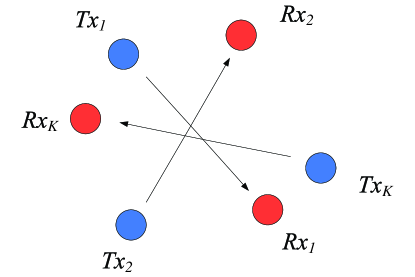
Figure 1: System model of a single cell.

As shown in Fig. 1, consider a set $\mathcal{K}=\{1,2,\ldots,K\}$ of wireless nodes and each node represents a transmitter-receiver pair (link). We define $Tx_{k}$ as the transmitter node of link $k$ and $Rx_{k}$ as the receiver node of link $k$. We first assume a single-cell wireless network, where every node can hear every other node in the network, and we will address the ad-hoc network scenario in Section IV.B. The system operates in discrete time with evenly spaced time slots [30][33]. We assume that all nodes always have a data packet to transmit at each time slot (i.e. we investigate the saturated traffic scenario), and the network is noise free and packet loss occurs only due to collision. The action of a node in this game is to select its transmission probability and a node $k$ will independently attempt transmission of a packet with transmit probability $p_{k}$. The action set available to node $k$ is $P_{k}=[0,1]$ for all $k\in\mathcal{K}$. Once the nodes decide their transmission probabilities based on which they transmit their packets, an action profile is determined. We denote the action profile in the random access game as a vector $\mathbf{p}=(p_{1},\ldots,p_{K})$ in $P=P_{1}\times\cdots\times P_{K}$. Then the throughput of node $k$ is given by

$$u_{k}(\mathbf{p})=p_{k}\prod_{i\in\mathcal{K}\backslash\{k\}}(1-p_{i}).$$ (1)

To capture the performance tradeoff in the network, the throughput (payoff) region is defined as $\mathscr{T}=\{(u_{1}(\textbf{p}),\ldots,u_{K}(\textbf{p}))|\ \exists\ \textbf{p}\in P\}$. The random access game can be formally defined by the tuple $\Gamma=\langle\mathcal{K},(P_{k}),(u_{k})\rangle$ [26]. Denote the transmission probability for all nodes but $k$ by $\mathbf{p}_{-k}=(p_{1},\ldots,p_{k-1},p_{k+1},\\ \ldots,p_{K})$. From (1), we can see that node $k$’s throughput depends not only on its own transmission probability $p_{k}$, but also the other nodes’ transmission probabilities $\mathbf{p}_{-k}$.

II-B Existing Solutions

The throughput tradeoff and stability of random access networks have been extensively studied from the game theoretic perspective [11]-[17]. This subsection briefly reviews these existing results and highlights the advantage and disadvantage of different approaches.

In the random access game, one of the most investigated problems is whether or not a Nash equilibrium exists. The definition of Nash equilibrium is given as follows [26].

Definition 1

A profile $\mathbf{p}$ of actions constitutes a Nash equilibrium of $\Gamma$ if $u_{k}(p_{k},\mathbf{p}_{-k})\geq u_{k}(p^{\prime}_{k},\mathbf{p}_{-k})$ for all $p^{\prime}_{k}\in P_{k}$ and $k\in\mathcal{K}$.

The NE of the investigated random access game has been addressed in the similar context of CSMA/CA networks where selfish nodes deliberately control their random deferment by altering their contention windows [14]. Specifically, the transmission probability $p_{k}$ in our model can be related to the contention window $CW_{k}$ in the CSMA/CA protocol, where $p_{k}=\frac{2}{1+CW_{k}}$. It has been shown in [14] that at the NE, at least one selfish node will set $CW_{k}=1$ (i.e. always transmit). If more than one selfish node sets its contention window to 1, it will cause zero throughput for all the nodes in the system. This kind of result is known as the tragedy of the commons. We can see that, myopic selfish behavior is detrimental in random access scenarios and novel mechanisms are required to encourage cooperative behavior among the self-interested devices. In addition, the existence of and convergence to the NE in random access games have been studied also in other scenarios, where individual nodes have utility functions that are different from (1) [11][12]. For example, the nodes in [11] adjust their transmission probabilities in an attempt to attain their desired throughputs. A local utility function is found for exponential backoff-based MAC protocols, based on which these protocols can be reverse-engineered in order to stabilize the network [12]. However, due to the inadequate coordination or feedback mechanism in these protocols, Pareto optimality of the throughput performance cannot be guaranteed.

Several recent works also investigate how to design new distributed algorithms that provably converge to the Pareto boundary of the network throughput region [14]-[16]. A distributed protocol is proposed in [14] to guide multiple selfish nodes to a Pareto-optimal NE by including penalties into their utility functions. However, the penalties must be carefully chosen. In [15], the utility maximization is solved using the dual decomposition technique by enabling nodes to cooperatively exchange coordination information among each other. Furthermore, it is shown in [16] that network utility maximization in random access networks can be achieved without real-time message passing among nodes. The key idea is to estimate the other nodes’ transmission probabilities from local observations, which in fact increases the internal computational overhead of individual nodes.

As discussed before, the goal of this paper is to design a simple distributed random access algorithm that requires limited information exchanges among nodes and also stabilizes the entire network. More importantly, this algorithm should be capable of achieving high efficiency and of differentiating among heterogeneous nodes carrying various traffic classes with different quality of service requirements. As we will show later, the game-theoretic concept of conjectural equilibrium provides such an elegant solution.

II-C Conjectural Equilibrium

In game-theoretic analysis, conclusions about the reached equilibria are based on assumptions about what knowledge the players possess. For example, the standard NE strategy assumes that every player believes that the other players’ actions will not change at NE. Therefore, it chooses to myopically maximize its immediate payoff [26]. Therefore, the players operating at equilibrium can be viewed as decision makers behaving optimally with respect to their beliefs about the strategies of other players.

To rigorously define CE, we need to include two new elements $\mathcal{S}$ and $s$ and, based on this, reformulate the random access game $\Gamma^{\prime}=\Big{(}\mathcal{K},(P_{k}),(u_{k}),(\mathcal{S}_{k}),(s_{k})\Big{)}$ [18]. $\mathcal{S}=\times_{k\in\mathcal{K}}\mathcal{S}_{k}$ is the state space, where $\mathcal{S}_{k}$ is the part of the state relevant to the node $k$. Specifically, the state in the random access game is defined as the contention probability that nodes experience. The utility function $u_{k}$ is a map from the nodes’ state space to real numbers, $u_{k}:\mathcal{S}_{k}\times P_{k}\rightarrow\mathcal{R}$. The state determination function $s=\times_{k\in\mathcal{K}}s_{k}$ maps joint action to state with each component $s_{k}:P\rightarrow\mathcal{S}_{k}$. Each node cannot directly observe the actions (transmission probabilities) chosen by the others, and each node has some belief about the state that would result from performing its available actions. The belief function $\tilde{s}_{k}$ is defined to be $\tilde{s}_{k}:P_{k}\rightarrow\mathcal{S}_{k}$ such that $\tilde{s}_{k}(p_{k})$ represents the state that node $k$ believes it would result in if it selects action $p_{k}$ . Notice that the beliefs are not expressed in terms of other nodes’ actions and preferences, and the multi-user coupling in these beliefs is captured directly by individual nodes forming conjectures of the effects of their own actions. Moreover, each node chooses the action $p_{k}\in P_{k}$ if it believes that this action will maximize its utility.

Definition 2

In the game $\Gamma^{\prime}$ defined above, a configuration of belief functions $(\tilde{s}_{1}^{*},\ldots,\tilde{s}_{K}^{*})$ and a joint action $p^{*}=(p_{1}^{*},\ldots,p_{K}^{*})$ constitute a conjectural equilibrium, if for each $k\in\mathcal{K}$,

$$\tilde{s}_{k}^{*}(p_{k}^{*})=s_{k}(p_{1}^{*},\ldots,p_{K}^{*})\ \textrm{and}\ p_{k}^{*}=\arg\max_{p_{k}\in P_{k}}u_{k}(\tilde{s}_{k}^{*}(p_{k}),p_{k}).$$

From the above definition, we can see that, at CE, all nodes’ expectations based on their beliefs are realized and each node behaves optimally according to its expectation. In other words, nodes’ beliefs are consistent with the outcome of the play and they behave optimally with respect to their beliefs. The key challenges are how to configure the belief functions such that reciprocal behavior is encouraged and how to design the evolution rules such that the network can dynamically converge to a CE having satisfactory performance. Section III provides bio-inspired solutions for these problems in random access games.

III Distributed Bio-inspired Learning

In this section, to promote reciprocity, we design a prescribed rule for each node to configure its belief about its expected contention of the wireless network as a linear function of its own transmission probability. It is shown that all the achievable operating points in the throughput region $\mathscr{T}$ are CE by deploying these belief functions. Furthermore, inspired by the biological mechanisms “derivative action” and “gradient dynamics”, we propose two distributed learning algorithms for these nodes to dynamically achieve the CE. We provide the sufficient conditions that guarantee the stability and convergence of the CE. We also discuss the similarities and differences between these bio-inspired algorithms and the existing well-known protocols. Finally, it is proven that any Pareto-inefficient operating point is a stable CE, i.e. we can approach arbitrarily close to the Pareto frontier of the throughput region $\mathscr{T}$.

III-A Individual Behavior

As discussed before, both the state space and belief functions need to be defined in order to investigate the existence of CE. In the random access game, we define the state $s_{k}=\prod_{i\in\mathcal{K}\backslash\{k\}}(1-p_{i})$ to be the contention measure signal representing the probability that all nodes except node $k$ do not transmit. This is because besides its own transmission probability, its throughput only depends on the probability that the remaining nodes do not transmit. We can see that state $s_{k}$ indicates the aggregate effects of the other nodes’ joint actions on node $k$’s payoff. In practice, it is hard for wireless nodes to compute the exact transmission probabilities of their opponents [16]. Therefore, we assume that $s_{k}$ is the only information that node $k$ has about the contention level of the entire network, because it is a metric that node $k$ can easily compute based on local observations. Specifically, from user $k$’s viewpoint, the probabilities of experiencing an idle time slot is $p_{k}^{idle}=(1-p_{k})s_{k}$. Let $n_{k}^{idle}$ denote the number of time slots between any two consecutive idle time slots. $n_{k}^{idle}$ has an independent identically distributed geometric distribution with probability $p_{k}^{idle}$. Therefore, we have $p_{k}^{idle}=1/(1+\bar{n}_{k}^{idle})$, where $\bar{n}_{k}^{idle}$ is the mean value of $n_{k}^{idle}$ and can be locally estimated by node $k$ through its observation of the channel contention history. Since node $k$ knows its own transmission probability $p_{k}$, it can estimate $s_{k}$ using $s_{k}=1/(1+\bar{n}_{k}^{idle})(1-p_{k})$. Notice that the action available to node $k$ is to choose the transmission probability $p_{k}\in P_{k}$. By the definition of belief function, we need to express the expected contention measure $\tilde{s}_{k}$ as a function of its own transmission probability $p_{k}$. The simplest approach is to deploy linear belief models, i.e. node $k$’s belief function takes the form

$$\tilde{s}_{k}(p_{k})=\bar{s}_{k}-a_{k}(p_{k}-\bar{p}_{k}),$$ (2)

for $k\in\mathcal{K}$. The values of $\bar{s}_{k}$ and $\bar{p}_{k}$ are specific states and actions, called reference points [25] and $a_{k}$ is a positive scalar. In other words, node $k$ assumes that other nodes will observe its deviation from its reference point $\bar{p}_{k}$ and the aggregate contention probability deviates from the referent point $\bar{s}_{k}$ by a quantity proportional to the deviation of $p_{k}-\bar{p}_{k}$. How to configure $\bar{s}_{k},\bar{p}_{k}$, and $a_{k}$ will be addressed in the rest of this paper. The reasons why we focus on the linear beliefs represented in (2) are two-fold. First, the linear form represents the simplest model based on which a user can model the impact of its environment. As we will show later in Section III-E, building and optimizing over such simple beliefs is sufficient for the network to achieve almost any operating point in the throughput region as a stable CE. Second, the conjecture functions deployed by the wireless users are based on the concept of reciprocity [5][7], which was developed in evolutionary biology, and refers to interaction mechanisms in which the evolution of cooperative behavior is favored by the probability of future mutual interactions. Similarly, in single-hop wireless networks, the devices repeatedly interact when accessing the channel. If they disregard the fact that they have a high probability to interact in the future, they will act myopically, which will lead to a tragedy of commons (the zero-payoff Nash equilibrium). However, if they recognize that their probability of interacting in the future is high, they will consider their impact on the network state, which is captured in the belief function by the positive $a_{k}$.

The goal of node $k$ is to maximize its expected throughput $p_{k}\cdot\tilde{s}_{k}(p_{k})$ taking into account the conjectures that it has made about the other nodes. Therefore, the optimization a node needs to solve becomes:

$$\max_{p_{k}\in P_{k}}p_{k}\Big{[}\bar{s}_{k}-a_{k}(p_{k}-\bar{p}_{k})\Big{]},$$ (3)

where the second term is the expected contention measure $\tilde{s}_{k}(p_{k})$ if node $k$ transmits with probability $p_{k}$. The product of $p_{k}$ and $\tilde{s}_{k}(p_{k})$ gives the expected throughput for $p_{k}\in P_{k}$. For $a_{k}>0$, node $k$ believes that increasing its transmission probability will increase its experienced contention probability. The optimal solution of (3) is given by

$$p_{k}^{*}=\min\Big{\{}\frac{\bar{s}_{k}}{2a_{k}}+\frac{\bar{p}_{k}}{2},1\Big{\}}.$$ (4)

In the following, we first show that forming simple linear beliefs in (2) can cause all the operating points in the achievable throughput region to be CE.

Theorem 1

All the operating points in the throughput region $\mathscr{T}$ are conjectural equilibria.

Proof: For each operating point $(\tau_{1},\ldots,\tau_{K})$ in the throughput region $\mathscr{T}$, there exists at least a joint action profile $(p^{*}_{1},\ldots,p^{*}_{K})\in P$ such that $\tau_{k}=u_{k}(\textbf{p}^{*})$, $\forall k\in\mathcal{K}$. We consider setting the parameters in the belief functions to be:

$$a_{k}^{*}=\frac{\prod_{i\in\mathcal{K}\backslash\{k\}}(1-p_{i}^{*})}{p_{k}^{*}}.$$ (5)

It is easy to check that, if the reference points are $\bar{s}_{k}=\prod_{i\in\mathcal{K}\backslash\{k\}}(1-p_{i}^{*}),\bar{p}_{k}=p_{k}^{*}$, we have $\tilde{s}_{k}(p_{k}^{*})=s_{k}(p_{1}^{*},\ldots,p_{K}^{*})$ and $p_{k}^{*}=\arg\max_{p_{k}\in P_{k}}u_{k}(\tilde{s}_{k}(p_{k}),p_{k})$. Therefore, this configuration of the belief functions and the joint action $\textbf{p}^{*}=(p_{1}^{*},\ldots,p_{K}^{*})$ constitute the CE that results in the throughput $(\tau_{1},\ldots,\tau_{K})$. $\blacksquare$

Theorem 1 establishes the existence of CE, i.e. for a particular $\textbf{p}^{*}\in P$, how to choose the parameters $\{\bar{s}_{k},\bar{p}_{k},a_{k}\}_{k=1}^{K}$ such that $\textbf{p}^{*}$ is a CE. However, it neither tells us how these CE can be achieved and sustained in the dynamic setting nor clarifies how different belief configurations can result in various CE.

In distributed learning scenarios, nodes learn when they modify their conjectures based on their new observations. Specifically, we first allow the nodes to revise their reference points based on their past local observations. Let $s_{k}^{t},p_{k}^{t},\tilde{s}_{k}^{t},\bar{s}_{k}^{t},\bar{p}_{k}^{t}$ be user $k$’s state, transmission probability, belief function, and reference points at stage $t$, in which $s_{k}^{t}=\prod_{i\in\mathcal{K}\backslash\{k\}}(1-p_{i}^{t})$. We propose a simple rule for individual nodes to update their reference points. At stage $t$, node $k$ set its $\bar{s}_{k}^{t}$ and $\bar{p}_{k}^{t}$ to be $s_{k}^{t-1}$ and $p_{k}^{t-1}$. In other words, node $k$’s conjectured utility function at stage $t$ is

$$u_{k}^{t}(\tilde{s}_{k}^{t}(p_{k}),p_{k})=p_{k}\Bigl{[}\prod_{i\in\mathcal{K}\backslash\{k\}}(1-p_{i}^{t-1})-a_{k}(p_{k}-p_{k}^{t-1})\Bigr{]}.$$ (6)

The remainder of this paper will investigate the dynamic properties of the resulting operating points and the performance trade-off among multiple competing nodes. In particular, for fixed $\{a_{k}\}_{k=1}^{K}$, Sections III-B and C will embed the above individual optimization scheme in two different distributed learning processes in which all the nodes update their transmission probabilities over time. Section III-E further allows individual nodes adaptively update their parameters $\{a_{k}\}_{k=1}^{K}$ such that desired efficiency can be attained. For given $\{a_{k}\}_{k=1}^{K}$, Section IV-A will derive a quantitative description of the resulting CE $\textbf{p}^{*}$.

III-B A Best Response Learning Algorithm

Our first algorithm in establishing reciprocity through a evolution process is inspired by the “derivative action”, which is a key component of biological motor control system models, e.g. cerebellar control over arm, hand, truncal, and leg movements [20][21]. Specifically, during limb movements, high frequency differential (velocity-like) signals after filtering due to biological sensors are attributed to lateral cerebellum as part of the input for cerebellar control. The classical control interpretation of “derivative action” is that the first-order derivative term serves as a short term prediction of the measured zero-order variable. For example, in a swing leg control, the velocity-like signals enable a cerebrocerebellar channel to better locate the ankle (or foot) position in front of the hip position during the swing phase. The conjecture-based approach is very similar in spirit with the aforementioned biological motor control models and the standard proportional integral derivative (PID) controllers in engineered systems [38]. In particular, the derivative term is substituted by a node’s internal belief of how its own action will impact the other nodes’ behavior. Our first learning algorithm adopts the simplest update mechanism in which each node adjusts its transmission probability using the best response that maximizes its conjectured utility function (6). Therefore, at stage $t$, node $k$ chooses a transmission probability

$$p_{k}^{t}=\arg\max_{p_{k}\in P_{k}}u_{k}^{t}(\tilde{s}_{k}^{t}(p_{k}),p_{k})=\min\Big{\{}\frac{p_{k}^{t-1}}{2}+\frac{\prod_{i\in\mathcal{K}\backslash\{k\}}(1-p_{i}^{t-1})}{2a_{k}},1\Big{\}}.$$ (7)

In this regard, the use of “derivative action” by an agent can be interpreted as using the best response to the forecasted effect of all the opponents’ strategies.

Algorithm 1 : A Distributed Best Response Learning Algorithm for Random Access

1:Initialize: $t=0$, the transmission probability $p_{k}^{0}\in[0,1]$, and the parameter $a_{k}>0$ in node $k$’s belief function, $\forall k\in\mathcal{K}$.

2:procedure 

3:     Locally at each node $k$, iterate through $t$:

4:     Set $t\leftarrow t+1.$

5:     for all $k\in\mathcal{K}$ do

6:         At stage $t$, $p_{k}^{t}\leftarrow\min\{p_{k}^{t-1}/2+\prod_{i\in\mathcal{K}\backslash\{k\}}(1-p_{i}^{t-1})/(2a_{k}),1\}$.

7:     end for

8:     Node $k$ decides if it will transmit data with a probability $p_{k}^{t}$ (or equivalently, maintain a window size of $CW_{k}^{t}=2/p_{k}^{t}-1$) for all the time slots during stage $t$.

9:end procedure

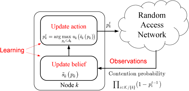
Figure 2: An illustration of the distributed learning process.

The detailed description of the entire distributed best response learning procedure is summarized in Algorithm 1 and it is also pictorially illustrated in Fig. 2. Next, we are interested in deriving the limiting behavior, e.g. stability and convergence, of this algorithm. For ease of illustration, the sufficient conditions for stability and convergence throughout this paper are expressed in terms of $\{p_{k}\}_{k=1}^{K}$ and $\{a_{k}\}_{k=1}^{K}$, respectively. The mapping from $\{p_{k}\}_{k=1}^{K}$ to $\{a_{k}\}_{k=1}^{K}$ is given in (5) and the mapping from $\{a_{k}\}_{k=1}^{K}$ to $\{p_{k}\}_{k=1}^{K}$ will be addressed in Section IV-A.

III-B1 Local Stability

Although Theorem 1 indicates that all the points in $\mathscr{T}$ are CE, they may not be necessarily stable. An unstable equilibrium is not desirable, because any small perturbation might cause the sequence of iterates to move away from the initial equilibrium. The following theorem describes a subset in $P$ in which all the points are stable CE.

Theorem 2

For any $\textbf{p}^{*}=(p_{1}^{*},\ldots,p_{K}^{*})\in P$, if

$$\sum_{k=1}^{K}p_{k}^{*}<1,\quad\textrm{or}\quad\sum_{i\in\mathcal{K}\backslash\{k\}}\frac{p_{k}^{*}}{1-p_{i}^{*}}<1,\ \forall k\in\mathcal{K},$$ (8)

$\textbf{p}^{*}$ is a stable CE for Algorithm 1.

Proof: To analyze the stability of different CE, we consider the Jacobian matrix of the self-mapping function in (7). Let $J_{ik}$ denote the element at row $i$ and column $k$ of the Jacobian matrix J. If $p_{k}^{t-1}/2+\prod_{i\in\mathcal{K}\backslash\{k\}}(1-p_{i}^{t-1})/(2a_{k})\leq 1$, the Jacobian matrix $\textbf{J}^{BR}$ of (7) is defined as:

$$J^{BR}_{ik}=\frac{\partial p_{i}^{t}}{\partial p_{k}^{t-1}}=\left\{\begin{array}[]{cl}\frac{1}{2},&\text{if $i=k$},\\ -\frac{1}{2a_{i}}\prod_{j\in\mathcal{K}\backslash\{i,k\}}(1-p_{j}^{t-1}),&\text{if $i\neq k$}.\end{array}\right.$$ (9)

As proven in Theorem 1, for $\textbf{p}^{*}=(p_{1}^{*},\ldots,p_{K}^{*})\in P$ to be a fixed point of the self-mapping function in (7), $a_{k}$ must be set to be $a_{k}^{*}=\prod_{i\in\mathcal{K}\backslash\{k\}}(1-p_{i}^{*})/p_{k}^{*}$. It follows that

$$J_{ik}^{BR}\rvert_{\textbf{p}=\textbf{p}^{*},\ \textbf{{a}}=\textbf{{a}}^{*}}=\left\{\begin{array}[]{cl}\frac{1}{2},&\text{if $i=k$},\\ -\frac{p_{i}^{*}}{2(1-p_{k}^{*})},&\text{if $i\neq k$}.\end{array}\right.$$ (10)

$\textbf{p}^{*}$ is stable if and only if the eigenvalues $\{\lambda_{k}\}_{k=1}^{K}$ of matrix $\textbf{J}^{BR}$ in (10) are all inside the unit circle of the complex plane, i.e. $|\lambda_{k}|<1,\forall k\in\mathcal{K}$.

From Gersgorin circle theorem [27], all the eigenvalues $\{\lambda_{k}\}_{k=1}^{K}$ of $\textbf{J}^{BR}$ are located in the region

$$\bigcup_{k=1}^{K}\Big{\{}|\lambda-J_{kk}^{BR}|\leqslant\sum_{i\in\mathcal{K}\backslash\{k\}}|J_{ik}^{BR}|\Big{\}}\ \textrm{and}\ \bigcup_{k=1}^{K}\Big{\{}|\lambda-J_{kk}^{BR}|\leqslant\sum_{i\in\mathcal{K}\backslash\{k\}}|J_{ki}^{BR}|\Big{\}}.$$

Note that $J_{kk}^{BR}=1/2$, these regions can be further simplified as

$$\bigcup_{k=1}^{K}\Big{\{}|\lambda-\frac{1}{2}|\leqslant\sum_{i\in\mathcal{K}\backslash\{k\}}\frac{p_{i}^{*}}{2(1-p_{k}^{*})}\Big{\}}\ \textrm{and}\ \bigcup_{k=1}^{K}\Big{\{}|\lambda-\frac{1}{2}|\leqslant\sum_{i\in\mathcal{K}\backslash\{k\}}\frac{p_{k}^{*}}{2(1-p_{i}^{*})}\Big{\}}.$$

If either condition in (8) is satisfied, all the eigenvalues of $\textbf{J}^{BR}$ must fall into the region $|\lambda-\frac{1}{2}|<\frac{1}{2}$, which is located within the unit circle $|\lambda|<1$. Therefore, $\textbf{p}^{*}$ is a stable CE.  $\blacksquare$

Remark 1

$p_{k}^{*}/(1-p_{i}^{*})$ can be interpreted as the worst case probability that node $k$ occupies the channel given that node $i$ does not transmit. This metric reflects from node $k$’s perspective the impact that node $i$’s evacuation has on the overall congestion of the channel. Therefore, the sufficient conditions in (8) means that if the system is not overcrowded from all the nodes’ perspectives, the corresponding CE is stable. We can see from Theorem 2 that lowering the transmission probabilities helps to stabilize the random access network. The system can accommodate a certain degree of individual nodes’ “aggressiveness” while maintaining the network stability. For example, if a node sends its packets with a probability close to 1, as long as the other nodes are conservative and they set their transmission probability small enough, the entire network can still be stabilized. However, if too many “aggressive” nodes with large transmission probabilities coexist, the system stability may collapse, leading to a tragedy of commons.

III-B2 Global Convergence

Note that Theorem 2 only investigates the stability for different fixed points, i.e. Algorithm 1 converges to these points when initial values are close enough to them. In addition to local stability, we are also interested in characterizing the global convergence of Algorithm 1 when using various $a_{k}$ to initialize the belief function $\tilde{s}_{k}$.

Theorem 3

Regardless of any initial value chosen for $\{p_{k}^{0}\}_{k=1}^{K}$, if the parameters $\{a_{k}\}_{k=1}^{K}$ in the belief functions $\{\tilde{s}_{k}\}_{k=1}^{K}$ satisfy

$$\sum_{i\in\mathcal{K}\backslash\{k\}}\frac{1}{a_{i}}<1,\forall k\in\mathcal{K},$$ (11)

Algorithm 1 converges to a unique CE.

Proof: For $a_{k}>1$, the self-mapping function in (7) can be rewritten as

$$p_{k}^{t}=\frac{p_{k}^{t-1}}{2}+\frac{\prod_{i\in\mathcal{K}\backslash\{k\}}(1-p_{i}^{t-1})}{2a_{k}}.$$ (12)

We can prove for Algorithm 1 the uniqueness of and the convergence to CE by showing that function (12) is a contraction map if the condition in (11) is satisfied.

Let $d(\cdot)$ be the induced distance function by certain vector norm in the Euclidean space. Consider two sequences of the transmission probability vectors $\{\textbf{p}^{0},\ldots,\textbf{p}^{t-1},\textbf{p}^{t},\ldots\}$ and $\{\hat{\textbf{p}}^{0},\ldots,\hat{\textbf{p}}^{t-1},\hat{\textbf{p}}^{t},\ldots\}$. We have

$$d(\textbf{p}^{t},\hat{\textbf{p}}^{t})=\lVert\textbf{p}^{t}-\hat{\textbf{p}}^{t}\rVert\leq\lVert\textbf{J}^{BR}\rVert\cdot\lVert\textbf{p}^{t-1}-\hat{\textbf{p}}^{t-1}\rVert=\lVert\textbf{J}^{BR}\rVert\cdot d(\textbf{p}^{t-1},\hat{\textbf{p}}^{t-1}).$$ (13)

The matrix norm used here is induced by the same vector norm. Using $\lVert\cdot\rVert_{1}$ for the Jacobian matrix of (12) as given in (10), we have

$$\lVert\textbf{J}^{BR}\rVert_{1}=\max_{k\in\mathcal{K}}\sum_{i=1}^{K}\lvert J_{ik}^{BR}\lvert\ \leq\frac{1}{2}+\frac{1}{2}\max_{k\in\mathcal{K}}\sum_{i\in\mathcal{K}\backslash\{k\}}\frac{1}{a_{i}}.$$ (14)

Therefore, if the condition in (11) is satisfied, there exist a constant $q\in[0,1)$ and a positive $\epsilon$, such that $q=\lVert\textbf{J}^{BR}\rVert_{1}=1-\epsilon<1$ and $\lVert\textbf{p}^{t}-\hat{\textbf{p}}^{t}\rVert_{1}\leq q\lVert\textbf{p}^{t-1}-\hat{\textbf{p}}^{t-1}\rVert_{1}$. From the contraction mapping theorem [28], the self-mapping function in (7) has a unique fixed point and the sequence $\{\textbf{p}^{t}\}_{t=0}^{+\infty}$ converges to the unique fixed point.  $\blacksquare$

Remark 2

We can also alternatively derive a sufficient condition using $\lVert\cdot\rVert_{\infty}$ for (13) to be a contraction map. We have

$$\lVert\textbf{J}^{BR}\rVert_{\infty}=\max_{k\in\mathcal{K}}\sum_{i=1}^{K}\lvert J_{ki}^{BR}\lvert\ \leq\frac{1}{2}+\frac{1}{2}\max_{k\in\mathcal{K}}\frac{K-1}{a_{k}}.$$ (15)

Therefore, if $a_{k}>K-1,\forall k\in\mathcal{K}$, Algorithm 1 also globally converges. However, it is easy to verify that it is a special case of the sufficient condition given by (11). In addition, we can see from (11) that, if the accumulated “aggressiveness” of the nodes in the entire networks reaches a certain threshold, the global convergence property may not hold. However, if all the nodes back off adequately by choosing their algorithm parameters $\{a_{k}\}_{k=1}^{K}$ such that condition (11) is satisfied, Algorithm 1 globally converges.

Remark 3

Under the sufficient condition in (11), by substituting (5) into (11), the limiting points lie in the set

$$\Big{\{}\textbf{p}^{*}=(p_{1}^{*},\ldots,p_{K}^{*})\Big{|}\sum_{i\in\mathcal{K}\backslash\{k\}}\frac{p_{i}^{*}}{\prod_{l\in\mathcal{K}\backslash\{i\}}(1-p_{l}^{*})}<1,\forall k\in\mathcal{K}\Big{\}}.$$ (16)

It is easy to check that this is a subset of $\{\textbf{p}^{*}=(p_{1}^{*},\ldots,p_{K}^{*})|\sum_{k=1}^{K}p_{k}^{*}<1\}$ for $K>2$, which verifies the intuition that the set that Algorithm 1 globally converges to should be a subset of the set of locally stable CE.

III-C A Gradient Play Learning Algorithm

The best-response based dynamics may lead to large fluctuations in the entire network, which may not be desirable if we want to avoid temporary system-wide instability. Therefore, in this subsection, we propose an alternative learning algorithm inspired by the gradient type dynamics, which has been well studied in the field of evolutionary biology [22][23]. For example, in population genetics, the evolutionary dynamics resulting for a particular mutant’s invasion fitness, i.e. its growth rate, are primarily governed by the fitness gradient. In other words, the population has a small probability of moving its phenotype [4] in the direction in which fitness is increasing, and this probability is proportional to the fitness gradient for possible mutants. This model has also been used to model fluid flow under a pressure gradient or the motion of organisms towards sites of higher nutrient concentration [24].

Motivated by the gradient dynamics, we consider the gradient play learning algorithm. At each iteration, each node updates its action gradually in the ascent direction of its conjectured utility function in (6). Specifically, at stage $t$, node $k$ chooses its transmission probability according to

$$p_{k}^{t}=\biggl{[}p_{k}^{t-1}+\gamma_{k}\frac{\partial u_{k}^{t}(\tilde{s}_{k}^{t}(p_{k}),p_{k})}{\partial p_{k}}\Biggr{\rvert}_{p_{k}=p_{k}^{t-1}}\biggr{]}_{0}^{1},$$ (17)

in which $[x]_{a}^{b}$ means $\max\{\min\{x,b\},a\}$. The engineering interpretation of this updating procedure is that each node will “mutate”, i.e. update its transmission probability, along the gradient direction of its conjectured utility function. As long as the stepsize $\gamma_{k}$ is small enough, the entire network will “evolve” smoothly and temporary system-wide instability will not occur. This algorithm also resembles the technique of exponential smoothing in statistics [39]. In the following, we assume that all nodes use the same stepsize $\gamma_{k}=\gamma,\forall k\in\mathcal{K}$ and $0<p_{k}^{t-1}<1$. If $\gamma$ is sufficiently small, substituting the utility function (6) into (17), we have

$$p_{k}^{t}=p_{k}^{t-1}+\gamma\Bigl{\{}\prod_{i\in\mathcal{K}\backslash\{k\}}(1-p_{i}^{t-1})-a_{k}p_{k}^{t-1}\Bigr{\}}.$$ (18)

The detailed description of the distributed gradient play learning mechanism is summarized in Algorithm 2. As for Algorithm 1, we investigate the stability and convergence of this gradient play learning algorithm.

Algorithm 2 : A Distributed Gradient Play Learning Algorithm for Random Access

1:Initialize: $t=0$, stepsize $\gamma$, the transmission probability $p_{k}^{0}\in[0,1]$, and the parameter $a_{k}>0$ in node $k$’s belief function, $\forall k\in\mathcal{K}$.

2:procedure 

3:     Locally at each node $k$, iterate through $t$:

4:     Set $t\leftarrow t+1.$

5:     for all $k\in\mathcal{K}$ do

6:         At stage $t$, $p_{k}^{t}\leftarrow\biggl{[}p_{k}^{t-1}+\gamma\Bigl{\{}\prod_{i\in\mathcal{K}\backslash\{k\}}(1-p_{i}^{t-1})-a_{k}p_{k}^{t-1}\Bigr{\}}\biggr{]}_{0}^{1}$.

7:     end for

8:     Node $k$ decides if it will transmit data with a probability $p_{k}^{t}$ (or equivalently, maintain a window size of $CW_{k}^{t}=2/p_{k}^{t}-1$) for all the time slots during stage $t$.

9:end procedure

III-C1 Local Stability

First of all, the following theorem describes a stable CE set in $P$ for Algorithm 2.

Theorem 4

For any $\textbf{p}^{*}=(p_{1}^{*},\ldots,p_{K}^{*})\in P$, if

$$\sum_{k=1}^{K}p_{k}^{*}<1,\quad\textrm{or}\quad\sum_{i\in\mathcal{K}\backslash\{k\}}\frac{p_{k}^{*}}{1-p_{i}^{*}}<1,\ \forall k\in\mathcal{K},$$ (19)

and the stepsize $\gamma$ is sufficiently small, $\textbf{p}^{*}$ is a stable CE for Algorithm 2.

Proof: Consider the Jacobian matrix $\textbf{J}^{GP}$ of the self-mapping function in (18). We have $J_{ik}^{GP}=\partial p_{i}^{t}/\partial p_{k}^{t-1}$. As discussed above, for $\textbf{p}^{*}=(p_{1}^{*},\ldots,p_{K}^{*})\in P$ to be a fixed point of the self-mapping function in (18), $a_{k}$ must be set to be $a_{k}^{*}=\prod_{i\in\mathcal{K}\backslash\{k\}}(1-p_{i}^{*})/p_{k}^{*}$. It follows that

$$J_{ik}^{GP}\rvert_{\textbf{p}=\textbf{p}^{*},\ \textbf{{a}}=\textbf{{a}}^{*}}=\left\{\begin{array}[]{cl}1-\gamma/p_{k}^{*}\cdot\prod_{l\in\mathcal{K}\backslash\{k\}}(1-p_{l}^{*}),&\text{if $i=k$},\\ -\gamma\prod_{l\in\mathcal{K}\backslash\{i,k\}}(1-p_{l}^{*}),&\text{if $i\neq k$}.\end{array}\right.$$ (20)

$\textbf{p}^{*}$ is stable if and only if the eigenvalues $\{\lambda_{k}\}_{k=1}^{K}$ of matrix $\textbf{J}^{GP}$ are all inside the unit circle of the complex plane, i.e. $|\lambda_{k}|<1,\forall k\in\mathcal{K}$. Recall that the spectral radius $\rho(\textbf{J})$ of a matrix J is the maximal absolute value of the eigenvalues[27]. Therefore, it is equivalent to prove that $\rho(\textbf{J}^{GP})<1$.

To a vector $\boldsymbol{w}=(w_{1},\cdots,w_{K})\in\mathcal{R}_{+}^{K}$ with positive entries, we associate a weighted $\ell_{\infty}$ norm, defined as

$$\|\boldsymbol{x}\|_{\infty}^{\boldsymbol{w}}=\max_{k\in\mathcal{K}}\frac{|x_{k}|}{w_{k}}.$$ (21)

The vector norm $\|\cdot\|_{\infty}^{\boldsymbol{w}}$ induces a matrix norm, defined by

$$\|A\|_{\infty}^{\boldsymbol{w}}=\max_{k\in\mathcal{K}}\frac{1}{w_{k}}\sum_{i=1}^{K}|a_{ki}|w_{i}.$$ (22)

According to Proposition A.20 in [31], $\rho(\textbf{J}^{GP})\leq\|\textbf{J}^{GP}\|_{\infty}^{\boldsymbol{w}}$. Consider the vector $\boldsymbol{w}=(w_{1},\cdots,w_{K})$ in which $w_{k}=p_{k}^{*}(1-p_{k}^{*})$. We have

$$\begin{split}\frac{1}{w_{k}}\sum_{i=1}^{K}|J_{ki}^{GP}|w_{i}&=1-\frac{\gamma\prod_{l\in\mathcal{K}\backslash\{k\}}(1-p_{l}^{*})}{p_{k}^{*}}+\sum_{i\in\mathcal{K}\backslash\{k\}}\frac{\gamma p_{i}^{*}\prod_{l\in\mathcal{K}\backslash\{k\}}(1-p_{l}^{*})}{p_{k}^{*}(1-p_{k}^{*})}\\ &=1-\frac{\gamma\prod_{l\in\mathcal{K}\backslash\{k\}}(1-p_{l}^{*})}{p_{k}^{*}}\Bigl{[}1-\sum_{i\in\mathcal{K}\backslash\{k\}}\frac{p_{i}^{*}}{1-p_{k}^{*}}\Bigr{]}.\end{split}$$ (23)

Therefore, if $\sum_{k\in\mathcal{K}}p_{k}^{*}<1,\ \forall k\in\mathcal{K}$, there exists some $\beta>0$ such that

$$\frac{\prod_{l\in\mathcal{K}\backslash\{k\}}(1-p_{l}^{*})}{p_{k}^{*}}\Bigl{[}1-\sum_{i\in\mathcal{K}\backslash\{k\}}\frac{p_{i}^{*}}{1-p_{k}}^{*}\Bigr{]}\geq\beta,\quad\forall k\in\mathcal{K}.$$ (24)

If the stepsize $\gamma$ satisfies $0<\gamma<1/\beta$, we have

$$\|\textbf{J}^{GP}\|_{\infty}^{\boldsymbol{w}}=\max_{k\in\mathcal{K}}\biggl{\{}1-\frac{\gamma\prod_{l\in\mathcal{K}\backslash\{k\}}(1-p_{l}^{*})}{p_{k}^{*}}\Bigl{[}1-\sum_{i\in\mathcal{K}\backslash\{k\}}\frac{p_{i}^{*}}{1-p_{k}^{*}}\Bigr{]}\biggr{\}}\leq 1-\gamma\beta<1.$$ (25)

Since $\rho(\textbf{J}^{GP})\leq\|\textbf{J}^{GP}\|_{\infty}^{\boldsymbol{w}}<1$, all the eigenvalues of $\textbf{J}^{GP}$ must fall into the unit circle $|\lambda|<1$. Therefore, $\textbf{p}^{*}$ is a stable CE. Similarly, by choosing $\boldsymbol{w}=[1,\cdots,1]$, we can show that, if

$$\sum_{i\in\mathcal{K}\backslash\{k\}}\frac{p_{k}^{*}}{1-p_{i}^{*}}<1,\ \forall k\in\mathcal{K},$$ (26)

and $\gamma$ is sufficiently small, $\textbf{p}^{*}$ is also stable. $\blacksquare$

III-C2 Global Convergence

Similarly as in the previous subsection, we derive in the following theorem a sufficient condition under which Algorithm 2 globally converges.

Theorem 5

Regardless of any initial value chosen for $\{p_{k}^{0}\}_{k=1}^{K}$, if the parameters $\{a_{k}\}_{k=1}^{K}$ in the belief functions $\{\tilde{s}_{k}\}_{k=1}^{K}$ satisfy

$$\sum_{i\in\mathcal{K}\backslash\{k\}}\frac{1}{a_{i}}<1,\forall k\in\mathcal{K},$$ (27)

and the stepsize $\gamma$ is sufficiently small, Algorithm 2 converges to a unique CE.

Proof: For the self-mapping function in (18), the elements of its Jacobian matrix $\textbf{J}^{GP}$ satisfy

$$J_{ik}^{GP}=\left\{\begin{array}[]{cl}1-\gamma a_{k},&\text{if $i=k$},\\ -\gamma\prod_{l\in\mathcal{K}\backslash\{i,k\}}(1-p_{l}),&\text{if $i\neq k$}.\end{array}\right.$$ (28)

Consider the induced distance by weighted $\ell_{\infty}$ norm in the Euclidean space. We have

$$\lVert\textbf{p}^{t}-\hat{\textbf{p}}^{t}\rVert_{\infty}^{\boldsymbol{w}}\leq\lVert\textbf{J}^{GP}\rVert_{\infty}^{\boldsymbol{w}}\cdot\lVert\textbf{p}^{t-1}-\hat{\textbf{p}}^{t-1}\rVert_{\infty}^{\boldsymbol{w}}.$$ (29)

Using $\boldsymbol{w}=(1/a_{1},\cdots,1/a_{K})$ for (29), we have

$$\lVert\textbf{J}^{GP}\rVert_{\infty}^{\boldsymbol{w}}=\max_{k\in\mathcal{K}}\biggl{\{}1-\gamma a_{k}+\sum_{i\in\mathcal{K}\backslash\{k\}}\prod_{l\in\mathcal{K}\backslash\{i,k\}}\frac{\gamma a_{k}(1-p_{l})}{a_{i}}\biggr{\}}\ \leq\max_{k\in\mathcal{K}}\biggl{\{}1-\gamma a_{k}\Bigl{(}1-\sum_{i\in\mathcal{K}\backslash\{k\}}\frac{1}{a_{i}}\Bigr{)}\biggr{\}}.$$ (30)

Therefore, if the condition in (27) is satisfied, there exists some $\beta>0$ such that

$$a_{k}\Bigl{(}1-\sum_{i\in\mathcal{K}\backslash\{k\}}\frac{1}{a_{i}}\Bigr{)}\geq\beta,\quad\forall k\in\mathcal{K}.$$ (31)

If the stepsize $\gamma$ satisfies $0<\gamma<1/\beta$, we have

$$\|\textbf{J}^{GP}\|_{\infty}^{\boldsymbol{w}}\leq\max_{k\in\mathcal{K}}\biggl{\{}1-\gamma a_{k}\Bigl{(}1-\sum_{i\in\mathcal{K}\backslash\{k\}}\frac{1}{a_{i}}\Bigr{)}\biggr{\}}\leq 1-\gamma\beta<1.$$ (32)

Therefore, there exist a constant $q\in[0,1)$ and a positive $\epsilon$, such that $q=\lVert\textbf{J}^{GP}\rVert_{\infty}^{\boldsymbol{w}}=1-\epsilon<1$ and $\lVert\textbf{p}^{t}-\hat{\textbf{p}}^{t}\rVert_{\infty}^{\boldsymbol{w}}\leq q\lVert\textbf{p}^{t-1}-\hat{\textbf{p}}^{t-1}\rVert_{\infty}^{\boldsymbol{w}}$. From the contraction mapping theorem [28], the self-mapping function in (18) has a unique fixed point and the sequence $\{\textbf{p}^{t}\}_{t=0}^{+\infty}$ converges to the unique fixed point.  $\blacksquare$

Remark 4

Compare Theorem 4 and 5 with Theorem 2 and 3. We can see that, given the same target operating point p or parameters $\{a_{k}\}_{k=1}^{K}$, Algorithm 2 exhibits similar properties in terms of local stability and global convergence, provided that its stepsize $\gamma$ is sufficiently small. In other words, the limiting behavior of these two distinct bio-inspired dynamic mechanisms are similar. However, we need to consider some design trade-off for both algorithms and choose the desired learning algorithm based on the specific system requirements about the speed of convergence and the performance fluctuation. Generally speaking, the best response learning algorithm converges fast, but it may cause temporary large fluctuations during the convergence process, which is not desirable for transporting constant-bit-rate applications. On the other hand, the gradient play learning algorithm with small stepsize will evolve smoothly at the cost of sacrificing its convergence rate.

III-D Alternative Interpretations of the Conjecture-based Learning Algorithms

In this section, we re-interpret the proposed algorithms using the the backoff mechanism model in which the transmission probabilities change from time slot to time slot [37], which helps us to understand the key difference between the proposed algorithms and 802.11 DCF. The superscript $t$ in this subsection represents the numbering of the time slots. We define $T_{k}^{t}$ and $T_{-k}^{t}$ as the events that node $k$ transmits data at time slot $t$ and any node in $\mathcal{K}\backslash\{k\}$ transmits data at time slot $t$, respectively. If $a_{k}>1$, the RHS of (7) equals to $\frac{p_{k}^{t-1}}{2}+\frac{\prod_{i\in\mathcal{K}\backslash\{k\}}(1-p_{i}^{t-1})}{2a_{k}}$, and the best response update function in (7) can be rewritten as

$$p_{k}^{t}=\frac{1}{2}\textrm{E}\{p_{k}^{t-1}\textbf{1}_{\{T_{-k}^{t-1}=1\}}|\textbf{p}^{t-1}\}+\frac{1}{2a_{k}}\textrm{E}\{\textbf{1}_{\{T_{-k}^{t-1}=0\}}\textbf{1}_{\{T_{k}^{t-1}=0\}}|\textbf{p}^{t-1}\}+\frac{1}{2}(1+\frac{1}{a_{k}})\textrm{E}\{\textbf{1}_{\{T_{-k}^{t-1}=0\}}\textbf{1}_{\{T_{k}^{t-1}=1\}}|\textbf{p}^{t-1}\},$$ (33)

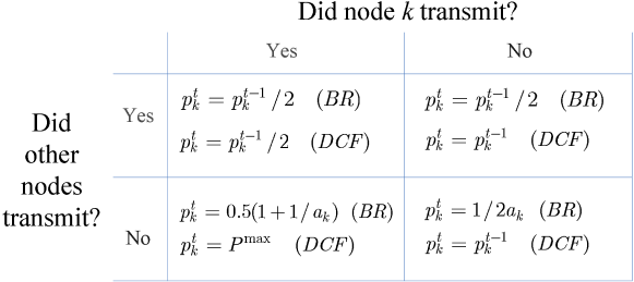
Figure 3: Comparison between the best response learning and the IEEE 802.11 DCF ($P^{\max}$ is specified in the DCF protocol).

where $\textbf{1}_{a}$ is an indicator function of event $a$ taking place, $\textrm{E}\{a|b\}$ is the expected value of $a$ given $b$, $\textrm{E}\{\textbf{1}_{\{T_{k}^{t-1}=1\}}|\textbf{p}^{t-1}\}=p_{k}^{t-1}$, and $\textrm{E}\{\textbf{1}_{\{T_{-k}^{t-1}=1\}}|\textbf{p}^{t-1}\}=1-\prod_{i\in\mathcal{K}\backslash\{k\}}(1-p_{i}^{t-1})$. According to (33), we can provide an alternative interpretation of the best-response update algorithm as follows. Consider the following update algorithm. At each time slot, if node $k$ observes that any other node attempts to transmit, i.e. it senses a busy channel, it reduces its transmission probability by a factor $1/2$. If no transmission attempt is made by any node in the system, node $k$ sets its transmission probability to be $1/2a_{k}$. Otherwise, if node $k$ makes a successful transmission, it will transmit with probability $0.5(1+1/a_{k})$ in the next time slot. We can see that equation (33) characterizes the expected trajectory of this alternative update mechanism. Fig. 3 compares this new interpretation with the IEEE 802.11 DCF [12]. We can see that, node $k$ behaves similarly in the best response algorithm and the IEEE 802.11 DCF if it made a transmission attempt in the previous time slot, and the fundamental difference between these two protocols is how node $k$ updates its action given that it did not transmit in the previous time slot. In DCF, $p_{k}^{t}$ is kept the same as $p_{k}^{t-1}$. However, as we can see from (33), the best response algorithm either performs back-off if the channel is busy or sets $p_{k}^{t}$ to be $1/2a_{k}$ if the channel is free. This can also be intuitively interpreted from a biological perspective: if the channel is busy, meaning that other competitors are accessing the resource (transmission opportunity), the node can avoid a confrontation by becoming less aggressive (i.e. reducing its transmission probability); if on the other hand, the system is idle and the resource is wasted, the node will consume the resource by increasing its transmission probability to $1/2a_{k}$.

Remark 5

Both Equation (5) and (33) intuitively explain the meaning of the algorithm parameters $\{a_{k}\}_{k=1}^{K}$. Note that the numerator of (5), $\prod_{i\in\mathcal{K}\backslash\{k\}}(1-p_{i}^{*})$, represents the probability that transmitter $k$ experiences a contention-free environment at $\textbf{p}^{*}$. The value of $1/a_{k}$, i.e. the ratio between node $k$’s transmission probability $p_{k}$ and its contention-free probability, indicates the “aggressiveness” of this particular node at equilibrium. In addition, according to (33), the transmission probability $1/2a_{k}$ also reflects node $k$’s “aggressiveness” in selecting its transmission probability after it sensed a free channel. It is straightforward to see the selection of $\{a_{k}\}_{k=1}^{K}$ introduces some trade-off between the stability and throughput of the networks. First of all, large values of $\{a_{k}\}_{k=1}^{K}$ refrain nodes from transmitting at a higher channel access probability, and hence, it stabilizes the system at the cost of reducing the throughput. On the other hand, lowering $\{a_{k}\}_{k=1}^{K}$ increases the nodes’ transmission probability, which may improve the throughput performance. However, it can cause the conditions in (8) and (19) to fail and the system becomes unstable. Therefore, the problems which we will investigate in the next subsection are which part of the throughput region can be achieved with stable CE and how the nodes can adaptively update their $\{a_{k}\}_{k=1}^{K}$ such that the system can attain efficient and stable operating points.

Before proceeding to the next subsection, similarly as for the best response algorithm, we present an reinterpretation of the gradient play. Equation (18) can be rewritten as

$$p_{k}^{t}=(1-\gamma a_{k})p_{k}^{t-1}\textrm{E}\{\textbf{1}_{\{T_{-k}^{t-1}=1\}}|\textbf{p}^{t-1}\}+[p_{k}^{t-1}+\gamma(1-a_{k}p_{k}^{t-1})]\textrm{E}\{\textbf{1}_{\{T_{-k}^{t-1}=0\}}|\textbf{p}^{t-1}\}.$$ (34)

If $a_{k}>1$, the interpretation of (34) is that at each time slot, if node $k$ senses a busy channel, it reduces its transmission probability by a factor $1-\gamma a_{k}$, otherwise it increases its transmission probability by an amount $\gamma(1-a_{k}p_{k}^{t-1})$. We can see that, this interpretation of the gradient play learning resembles the well-known AIMD (Additive Increase Multiplicative Decrease) control algorithm, which has been widely applied in the context of congestion avoidance in computer networks due to its superior performance in terms of convergence and efficiency [29].

III-E Stability of the Throughput Region

The results in the previous subsections describe the values of $\{p_{k}\}_{k=1}^{K}$ and $\{a_{k}\}_{k=1}^{K}$ for which local stability and global convergence can be guaranteed in both Algorithm 1 and 2. This subsection directly investigates for both algorithms the stability of achievable operating points in the throughput region $\mathscr{T}$.

Lemma 6

The Pareto boundary of the throughput region $\mathscr{T}$ is the set of all points $\boldsymbol{\tau}=(\tau_{1},\ldots,\tau_{K})$ such that $\tau_{k}=p_{k}\prod_{i\in\mathcal{K}\backslash\{k\}}(1-p_{i})$ where $\textbf{p}=(p_{1},\ldots,p_{K})$ is a vector satisfying $\textbf{p}\geqslant\textbf{0}$ and $\sum_{k\in\mathcal{K}}p_{k}=1$; and each such $\boldsymbol{\tau}$ is determined by a unique such p.

Proof: See Theorem 1 in [30].  $\blacksquare$

Theorem 7

Regardless of the number of nodes in the network, for any Pareto-inefficient operating point $\boldsymbol{\tau}^{*}$ in the throughput region $\mathscr{T}$, there always exists a belief configuration $\{a_{k}\}_{k=1}^{K}$ stabilizing Algorithm 1 and 2, and achieve the throughput $\boldsymbol{\tau}^{*}$. If $K>2$, any Pareto-optimal operating point $\{p_{k}^{*}\}_{k=1}^{K}$ in $\mathscr{T}$ that satisfies $p_{k}^{*}>0,\forall k\in\mathcal{K}$ is a stable CE for Algorithm 1 and 2.

Proof: From Theorem 2, we know that $\sum_{k\in\mathcal{K}}p_{k}<1$ is sufficient to guarantee that the corresponding CE is stable. Therefore, it is equivalent to check that any Pareto-inefficient operating point $\boldsymbol{\tau}^{*}$ can be achieved with a joint transmission probability $\textbf{p}^{*}\in P$ satisfying $\sum_{k\in\mathcal{K}}p_{k}^{*}<1$.

Define the throughput region

$$\mathscr{T}(t)=\{(u_{1}(\textbf{p}),\ldots,\\ u_{K}(\textbf{p}))|\ \exists\ \textbf{p}\in P,\sum_{k\in\mathcal{K}}p_{k}\leq t\},$$ (35)

in which an additional constraint $\sum_{k\in\mathcal{K}}p_{k}\leq t$ is imposed. We denote the Pareto boundary of $\mathscr{T}(t)$ as

$$\partial\mathscr{T}(t)=\{\boldsymbol{\tau}|\ \nexists\ \boldsymbol{\tau}^{\prime}\in\mathscr{T}(t)\ \textrm{such that}\ \tau^{\prime}_{k}\geq\tau_{k},\ \forall k\in\mathcal{K}\ \textrm{and}\ \tau^{\prime}_{k}>\tau_{k},\ \exists k\in\mathcal{K}\}.$$ (36)

Following the proof of Lemma 6, we can draw a similar conclusion: all the points on $\partial\mathscr{T}(t)$ satisfy $\sum_{k\in\mathcal{K}}p_{k}=t$. By Lemma 6, $\partial\mathscr{T}(1)$ corresponds to the Pareto boundary of $\mathscr{T}$. Note that $\partial\mathscr{T}(0)=\textbf{0}$. In other words, varying $t$ from 1 to 0 will cause $\partial\mathscr{T}(t)$ to continuously shrink from the Pareto boundary of the throughput region $\mathscr{T}$ to the origin 0. Therefore, for any Pareto inefficient point $\boldsymbol{\tau}^{*}\in\mathscr{T}$, there exists $0\leq t^{\prime}<1$ such that $\boldsymbol{\tau}^{*}$ lie on $\partial\mathscr{T}(t^{\prime})$, i.e. $\boldsymbol{\tau}^{*}$ can be achieved with an action profile $\textbf{p}^{*}$ satisfying $\sum_{k\in\mathcal{K}}p_{k}^{*}=t<1$.

To prove the Pareto boundary are stable CE when $K>2$, we need to show that the eigenvalues $\{\xi_{n}^{BR}\}_{n=1}^{N}$ of the Jacobian matrices $\textbf{J}^{BR}$ and $\textbf{J}^{GP}$ are all inside the unit circle of the complex plane [28], i.e. $|\xi_{n}|<1,\forall n\in\mathcal{N}$. Take the best response dynamics for example. To determine the eigenvalues of $\textbf{J}^{BR}$, we have

$$\begin{split}\det(\xi I-\textbf{J}^{BR})&=\left|\begin{array}[]{cccc}\xi-\frac{1}{2}&\frac{p_{1}}{2(1-p_{2})}&\ldots&\frac{p_{1}}{2(1-p_{K})}\\ \frac{p_{2}}{2(1-p_{1})}&\xi-\frac{1}{2}&\ldots&\frac{p_{2}}{2(1-p_{K})}\\ \vdots&\vdots&\ddots&\vdots\\ \frac{p_{K}}{2(1-p_{1})}&\frac{p_{K}}{2(1-p_{2})}&\ldots&\xi-\frac{1}{2}\\ \end{array}\right|\\ &=\left|\begin{array}[]{cccc}\xi-\frac{1}{2}&\frac{p_{1}}{2(1-p_{2})}&\ldots&\frac{p_{1}}{2(1-p_{K})}\\ \frac{p_{2}}{2(1-p_{1})}-\frac{p_{2}}{p_{1}}\bigl{(}\xi-\frac{1}{2}\bigr{)}&\xi-\frac{1}{2}-\frac{p_{2}}{2(1-p_{2})}&\ldots&0\\ \vdots&\vdots&\ddots&\vdots\\ \frac{p_{K}}{2(1-p_{1})}-\frac{p_{K}}{p_{1}}\bigl{(}\xi-\frac{1}{2}\bigr{)}&0&\ldots&\xi-\frac{1}{2}-\frac{p_{K}}{2(1-p_{K})}\\ \end{array}\right|\\ &=\left|\begin{array}[]{cccc}\bigl{(}\xi-\frac{1}{2}-\frac{p_{1}}{2(1-p_{1})}\bigr{)}\cdot\bigl{[}1+\sum_{k=1}^{K}\frac{\frac{p_{k}}{2(1-p_{k})}}{\xi-\frac{1}{2}-\frac{p_{k}}{2(1-p_{k})}}\bigr{]}&0&\ldots&0\\ \frac{p_{2}}{2(1-p_{1})}-\frac{p_{2}}{p_{1}}\bigl{(}\xi-\frac{1}{2}\bigr{)}&\xi-\frac{1}{2}-\frac{p_{2}}{2(1-p_{2})}&\ldots&0\\ \vdots&\vdots&\ddots&\vdots\\ \frac{p_{K}}{2(1-p_{1})}-\frac{p_{K}}{p_{1}}\bigl{(}\xi-\frac{1}{2}\bigr{)}&0&\ldots&\xi-\frac{1}{2}-\frac{p_{K}}{2(1-p_{K})}\\ \end{array}\right|.\end{split}$$

Therefore, we can see that, the eigenvalues of $\textbf{J}^{BR}$ are the roots of

$$\bigl{[}1+\sum_{k=1}^{K}\frac{\frac{p_{k}}{2(1-p_{k})}}{\xi-\frac{1}{2}-\frac{p_{k}}{2(1-p_{k})}}\bigr{]}\cdot\prod_{k=1}^{K}\bigl{(}\xi-\frac{1}{2}-\frac{p_{k}}{2(1-p_{k})}\bigr{)}=0.$$ (37)

Denote $f(\xi)=\sum_{k=1}^{K}\frac{\frac{p_{k}}{2(1-p_{k})}}{\xi-\frac{1}{2}-\frac{p_{k}}{2(1-p_{k})}}$. First, we assume that $p_{i}\neq p_{j},\forall i,j$. Without loss of generality, consider $p_{1}<p_{2}<\cdots<p_{K}$. In this case, the eigenvalues of $\textbf{J}^{BR}$ are the roots of $f(\xi)=-1$. Note that $f(\xi)$ is a continuous function and it strictly decreases in $(-\infty,\frac{1}{2}+\frac{p_{1}}{2(1-p_{1})})$, $(\frac{1}{2}+\frac{p_{1}}{2(1-p_{1})},\frac{1}{2}+\frac{p_{2}}{2(1-p_{2})})$, $\cdots$, $(\frac{1}{2}+\frac{p_{K-1}}{2(1-p_{K-1})},\frac{1}{2}+\frac{p_{K}}{2(1-p_{K})})$, and $(\frac{p_{K}}{2(1-p_{K})},+\infty)$. We also have $\lim_{\xi\rightarrow(\frac{1}{2}+\frac{p_{k}}{2(1-p_{k})})^{-}}f(\xi)=-\infty$, $\lim_{\xi\rightarrow(\frac{1}{2}+\frac{p_{k}}{2(1-p_{k})})^{+}}f(\xi)=+\infty,n=1,2,\cdots,K$, and $\lim_{\xi\rightarrow-\infty}f(\xi)=\lim_{\xi\rightarrow+\infty}f(\xi)=0$. Therefore, the roots of $f(\xi)=-1$ lie in $(-\infty,\frac{1}{2}+\frac{p_{1}}{2(1-p_{1})})$, $(\frac{1}{2}+\frac{p_{1}}{2(1-p_{1})},\frac{1}{2}+\frac{p_{2}}{2(1-p_{2})})$, $\cdots$, $(\frac{1}{2}+\frac{p_{K-1}}{2(1-p_{K-1})},\frac{1}{2}+\frac{p_{K}}{2(1-p_{K})})$ respectively.

For the operating points on the Pareto boundary, we have $\sum_{k=1}^{K}p_{k}=1$. It is easy to verify that $f(0)=-1$, i.e. $\xi_{1}=0$. Therefore,

$$\rho(\textbf{J}^{BR})=\max_{k}|\xi_{k}|=\xi_{K}\in(\frac{1}{2}+\frac{p_{K-1}}{2(1-p_{K-1})},\frac{1}{2}+\frac{p_{K}}{2(1-p_{K})}).$$ (38)

To see $\xi_{K}<1$ for $0\leq p_{1}<p_{2}<\cdots<p_{K}$ and $\sum_{k=1}^{K}p_{k}=1$. We differentiate two cases:

1) If $p_{K}\leq 0.5$, we have $\xi_{K}<\frac{1}{2}+\frac{p_{K}}{2(1-p_{K})}\leq 1$;

2) If $p_{K}>0.5$, we have $\frac{1}{2}+\frac{p_{K-1}}{2(1-p_{K-1})}<1$ and $\frac{1}{2}+\frac{p_{K}}{2(1-p_{K})}>1$. Since $f(\xi)$ strictly decreases in $(\frac{1}{2}+\frac{p_{K-1}}{2(1-p_{K-1})},\frac{1}{2}+\frac{p_{K}}{2(1-p_{K})})$, we have $\rho(\textbf{J}^{BR})<1$ if and only if $f(1)<-1$. In fact,

$$f(1)-(-1)=\sum_{k=1}^{K}\frac{p_{k}}{1-2p_{k}}+1=\sum_{k=1}^{K-1}p_{k}\bigl{(}\frac{1}{1-2p_{k}}-\frac{1}{1-2\sum_{m=1}^{K-1}p_{m}}\bigr{)}<0.$$ (39)

The inequality holds because $\frac{1}{1-2p_{k}}<\frac{1}{1-2\sum_{m=1}^{K-1}p_{m}}$ for $k=1,2,\ldots,K-1$ when $p_{K}>0.5$, $0\leq p_{1}<p_{2}<\cdots<p_{K}$, and $\sum_{k=1}^{K}p_{k}=1$.

Second, we consider the cases in which there exists $p_{i}=p_{j}$ for certain $i,j$. Suppose that $\{p_{k}\}_{k=1}^{K}$ take $M$ discrete values $\kappa_{1},\cdots,\kappa_{M}$ and the number of $\{p_{k}\}_{k=1}^{K}$ that equal to $\kappa_{m}$ is $n_{m}$. In this case, Equation (37) is reduced to

$$\bigl{[}1+\sum_{k=1}^{K}\frac{\frac{p_{k}}{2(1-p_{k})}}{\xi-\frac{1}{2}-\frac{p_{k}}{2(1-p_{k})}}\bigr{]}\cdot\prod_{m=1}^{M}\bigl{(}\xi-\frac{1}{2}-\frac{\kappa_{m}}{2(1-\kappa_{m})}\bigr{)}^{n_{m}}=0.$$ (40)

Hence, equation $f(\xi)=-1$ has $K+M-\sum_{k=1}^{M}n_{m}$ roots in total, and $\xi=\frac{1}{2}+\frac{\kappa_{m}}{2(1-\kappa_{m})}$ is a root of multiplicity $n_{m}-1$, $\forall m$. All these roots are the eigenvalues of matrix $\textbf{J}^{BR}$. Similarly, the remaining roots of $f(\xi)=-1$ lie in $(-\infty,\frac{1}{2}+\frac{\kappa_{1}}{2(1-\kappa_{1})})$, $(\frac{1}{2}+\frac{\kappa_{1}}{2(1-\kappa_{1})},\frac{1}{2}+\frac{\kappa_{2}}{2(1-\kappa_{2})})$, $\cdots$, $(\frac{1}{2}+\frac{\kappa_{M-1}}{2(1-\kappa_{M-1})},\frac{1}{2}+\frac{\kappa_{M}}{2(1-\kappa_{M})})$. If $K>2$, $\sum_{k=1}^{K}p_{k}=1$ is still sufficient to guarantee that $f(1)<-1$. Therefore, $|\xi_{k}^{BR}|<1,\forall k\in\mathcal{K}$. $\blacksquare$

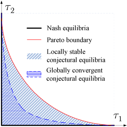
Figure 4: Comparison among different solution concepts.

Fig. 4 compares the throughput performance among various game-theoretic solution concepts, including Nash equilibria, Pareto frontier, locally stable conjectural equilibria, and globally convergent conjectural equilibria, in random access games. As proven in Theorem 7, Fig. 4 shows that, the entire space spanning between the Nash equilibria and Pareto frontier essentially consists of stable conjectural equilibria. In addition, as discussed in Remark 3, the set of globally convergent CE is a subset of the stable CE set.

In practice, it is more important to construct algorithmic mechanisms to attain the desirable CE that operate stably and closely to the Pareto boundary. To this end, we develop an iterative algorithm and summarize it as Algorithm 3. Specifically, this algorithm has an inner loop and an outer loop. The inner loop adopts either Algorithm 1 or 2 to achieve convergence for fixed $\{a_{k}\}_{k=1}^{K}$. This algorithm initializes $a_{k}>|\mathcal{K}|$ such that it initially globally converges. After converging to a stable CE, the outer loop adaptively adjusts $\{a_{k}\}_{k=1}^{K}$ until desired efficiency is attained. The outer loop updates $\{a_{k}\}_{k=1}^{K}$ in the multiplicative manner due to two reasons. First, reducing $\{a_{k}\}_{k=1}^{K}$ individually increases $\{p_{k}^{t}\}_{k=1}^{K}$ and $\sum_{k=1}^{K}p_{k}$ and hence, moves the operating point towards the Pareto boundary. Second, multiplying $\{a_{k}\}_{k=1}^{K}$ by the same discount factor can maintain weighted fairness among different nodes. Both reasons will be analytically explained in the Section IV. It is also worth mentioning that individual nodes can measure the Pareto efficiency in a fully distributed manner during the outer loop iteration. For example, individual nodes can estimate the other nodes’ transmission probabilities $\{p_{k}^{t}\}_{k=1}^{K}$ based on its local observation and figure out whether the current operating point is close to the Pareto boundary by calculating $\sum_{k\in\mathcal{K}}p_{k}^{t}$ [16]. When the network size grows bigger, individually estimating different nodes’ transmission probabilities becomes challenging. An alternative solution is that individual nodes can instead monitor their common observation of the aggregate throughput $\sum_{k\in\mathcal{K}}u_{k}^{t}$ and terminate the update of $\{a_{k}\}_{k=1}^{K}$ once the aggregate throughput starts to decrease. Next, we discuss several implementation issues regarding Algorithm 3. First, it is not necessary that all the nodes update their parameters $\{a_{k}\}_{k=1}^{K}$ synchronously. However, these nodes need to maintain the same update frequency, e.g. each node will update its parameter after a certain number of timeslots or seconds. As long as $\delta$ is small, the performance gap between the actual CE and the intended one will not be large. Moreover, in order to guarantee fairness, the new incoming nodes need to know the real-time parameters of the old nodes in the same traffic class. This initialization only needs to be done once, when the new nodes enter the cell by tracking the evolution of the transmission probabilities of the nodes in the same traffic class.

Algorithm 3 : Adaptive Distributed Learning Algorithm for Random Access

1:Initialize: stepsize $\gamma$ and $\delta$, the transmission probability $p_{k}^{0}\in[0,1]$, and the parameter $a_{k}>|\mathcal{K}|$ in node $k$’s belief function, $\forall k\in\mathcal{K}$.

2:procedure 

3:     outer loop: For each node $k$, $a_{k}\leftarrow a_{k}(1-\delta)$.

4:      inner loop: Locally at each node $k$, use Algorithm 1 or 2 to update $p_{k}^{t}$.

5:      until it converges.

6:     until the aggregate throughput is maximized or $\sum_{k\in\mathcal{K}}p_{k}^{t}\approx 1$.

7:end procedure

IV Extensions to Heterogeneous Networks and Ad-hoc Networks

In this section, we first investigate how users with different qualify-of-service requirements should initialize their belief functions and interact in the heterogeneous network setting and show that the conjecture-based approaches approximately achieve the weighted fairness. Furthermore, we discuss how the single-cell solution can be extended to the general ad-hoc network scenario, where only the devices within a certain neighborhood range will impact each other’s throughput.

IV-A Equilibrium Selection for Heterogeneous Networks

Consider a network with $N>1$ different classes of nodes. Let $\phi_{n}$ denote the parameter that class-$n$ nodes choose for their conjectured utility functions (i.e. the parameter $a_{k}$ if node $k$ belongs to class-$n$) and $\mathcal{F}_{n}$ denote the set of nodes that set their algorithm parameters to be $\phi_{n}$, $1\leq n\leq N$. At equilibrium, the transmission probabilities of the same class of nodes are equal, denoted as $\tilde{p}_{n}$. Before we proceed, we first define the weighted fairness for the random access game [32]. For each traffic class $n$, we associate with a positive weight $\chi_{n}$. Then the weighted fairness intended for the random access game satisfy

$$\forall i,j\in\{1,2,\cdots,N\},\forall s\in\mathcal{F}_{i},\forall s^{\prime}\in\mathcal{F}_{j},\frac{\textrm{E}\{\textbf{1}_{\{T_{-s}=0\}}\textbf{1}_{\{T_{s}=1\}}\}}{\chi_{i}}=\frac{\textrm{E}\{\textbf{1}_{\{T_{-s^{\prime}}=0\}}\textbf{1}_{\{T_{s^{\prime}}=1\}}\}}{\chi_{j}},$$ (41)

which means that the probability of an successful transmission attempt for traffic class $n$ is proportional to its weight $\chi_{n}$. By simple manipulation, we have the equivalent form for equation (41) [32]:

$$\forall i,j\in\{1,2,\cdots,N\},\frac{p_{i}^{WF}}{(1-p_{i}^{WF})\chi_{i}}=\frac{p_{j}^{WF}}{(1-p_{j}^{WF})\chi_{j}}.$$ (42)

Recall that Theorem 1 showed how to choose $\{a_{k}\}_{k=1}^{K}$ given a desired operating point $\{p_{k}^{*}\}_{k=1}^{K}$ such that it is a CE. The following theorem indicates the quantitative relationship between the chosen algorithm parameters $\{\phi_{n}\}_{n=1}^{N}$, the sizes of different classes $\{\mathcal{F}_{n}\}_{n=1}^{N}$, and the resulting steady-state transmission probabilities $\{\tilde{p}_{n}\}_{n=1}^{N}$. More importantly, it also shows that if the network size is large, the conjecture-based algorithms approximately achieve weighted fairness.

Theorem 8

Suppose that $\phi_{n}\geq 2,\ \forall 1\leq n\leq N$. The achieved steady-state transmission probabilities $\{\tilde{p}_{n}\}_{n=1}^{N}$ are given by

$$\tilde{p}_{n}=\frac{1}{2}\bigg{(}1-\sqrt{1-\frac{4\varrho}{\phi_{n}}}\bigg{)},$$ (43)

where $\varrho$ satisfies

$$\varrho=\frac{1}{2^{K}}\prod_{n=1}^{N}\bigg{[}\bigg{(}1+\sqrt{1-\frac{4\varrho}{\phi_{n}}}\bigg{)}^{|\mathcal{F}_{n}|}\bigg{]}.$$ (44)

Proof: As shown in Theorem 1, $a_{k}^{*}p_{k}^{*}=\prod_{i\in\mathcal{K}\backslash\{k\}}(1-p_{i}^{*})$. Denote $\varrho=\prod_{i\in\mathcal{K}}(1-\tilde{p}_{i})$. Therefore, we obtain

$$\phi_{n}\tilde{p}_{n}(1-\tilde{p}_{n})=\varrho,\ \forall\ 1\leq n\leq N.$$ (45)

Since $\phi_{n}>2$, we have $\tilde{p}_{n}<0.5$. Such a root of the quadratic equation in (45) is given in (43). Note that $\varrho=\prod_{i\in\mathcal{K}}(1-\tilde{p}_{i})$. Substituting (43) into this equality, we get (44).

We can verify that a unique $\varrho$ satisfying the equality in (44) exists if $\phi_{n}\geq 2,\ \forall 1\leq n\leq N$. This is because the RHS of (44) is feasible for $\varrho\leq\textrm{min}_{1\leq n\leq N}\{\phi_{n}\}/4$ and it is a strictly decreasing function in $\varrho$. Meanwhile, the LHS of (44) is strictly increasing on $\varrho\in[0,\textrm{min}_{1\leq n\leq N}\{\phi_{n}\}/4]$. Note that when $\varrho=\textrm{min}_{1\leq n\leq N}\{\phi_{n}\}/4$,

$$\textrm{LHS of (\ref{eq:eqn39})}=\min_{1\leq n\leq N}\frac{\phi_{n}}{4}\geq\frac{1}{2}\geq\textrm{RHS of (\ref{eq:eqn39})}.$$ (46)

if $\phi_{n}\geq 2$. Therefore, a unique $\varrho\in[0,\textrm{min}_{1\leq n\leq N}\{\phi_{n}\}/4]$ satisfies (44) exists. $\blacksquare$

Remark 6

There are several intuitions and observations that we can obtain from Theorem 8. First, the multiplicative decreasing update in Algorithm 3 aims to move the operating points towards Pareto boundary. A quantitative approximation between the steady-state transmission probability $\tilde{p}_{n}$ and the algorithm parameter $\phi_{n}$ of each traffic class can be derived if a large number of nodes coexist. Since $\varrho\rightarrow 0$ when $|\mathcal{F}_{n}|$ is large, using the Taylor expansion, $\tilde{p}_{n}$ can be approximated as $\varrho/\phi_{n}$, i.e. the steady-state transmission probability $\tilde{p}_{n}$ decays as the inverse first power of parameter $\phi_{n}$ that indicates the “aggressiveness” of traffic class $n$. Finally, we also observe from (45) that, if $|\mathcal{F}_{n}|$ is large, $\tilde{p}_{n}\rightarrow 0$ and $1-\tilde{p}_{n}\approx 1$. Therefore,

$$\forall i,j\in\{1,2,\cdots,N\},\phi_{i}\tilde{p}_{i}(1-\tilde{p}_{i})=\phi_{j}\tilde{p}_{j}(1-\tilde{p}_{j})\Rightarrow\frac{\phi_{i}\tilde{p}_{i}}{1-\tilde{p}_{i}}\approx\frac{\phi_{j}\tilde{p}_{j}}{1-\tilde{p}_{j}}.$$ (47)

Equation (47) indicates that Algorithm 1 and 2 approximately achieve weighted fairness given in (42) with weight $\chi_{n}=1/\phi_{n}$. Moreover, it is worth mentioning that the weighted fairness is purely an implicit by-product of the conjecture-based approach and it can be sustained with stability. Therefore, Algorithm 3 chooses to multiply $\{a_{k}\}_{k=1}^{K}$ by the same discount factor $1-\delta$ such that the weighted fairness can be maintained.

IV-B Extension to Ad-hoc Networks

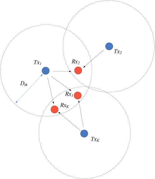
Figure 5: System model of ad hoc networks.

Consider a wireless ad-hoc network with a set $\mathcal{K}=\{1,2,\ldots,K\}$ of distinct node pairs in Fig. 5. Each link (node pair) consists of one dedicated transmitter and one dedicated receiver. We assume that the transmission of a link is interfered from the transmission of another link, if the distance between the receiver node of the former and the transmitter node of the latter is less than some threshold $D_{th}$ [9][15]. For any node $i$, we define $I_{i}\subseteq\mathcal{K}$ as the set of nodes whose transmitters cause interference to the receiver of node $i$ and $O_{i}\subseteq\mathcal{K}$ as the set of nodes whose receivers get interfered from the transmitter of node $i$. For example, in Fig. 5, $I_{1}=\{K\}\ \textrm{and}\ O_{1}=\{2,K\}$. Then, the throughput of node $i$ is

$$u_{k}(\mathbf{p})=p_{k}\prod_{i\in I_{k}}(1-p_{i}).$$ (48)

In this scenario, the state, namely, the contention measure signal, can be redefined according to $s_{k}=\prod_{i\in I_{k}}(1-p_{i})$. Applying the conjecture-based approach, we have the following conjectured utility function for node $k$:

$$u_{k}^{t}(\tilde{s}_{k}^{t}(p_{k}),p_{k})=p_{k}\Bigl{[}\prod_{i\in I_{k}}(1-p_{i}^{t-1})-a_{k}(p_{k}-p_{k}^{t-1})\Bigr{]}.$$ (49)

Parallel to the theorems proven in Section III-B and C, we have the following theorems on the stability and convergence of conjecture-based bio-inspired learning algorithms in ad-hoc networks. These theorems can be shown similarly as in Section III, and hence, the proofs are omitted.

IV-B1 Stability and Convergence

Theorem 9

For any $\textbf{p}^{*}=(p_{1}^{*},\ldots,p_{K}^{*})\in P$, if

$$\sum_{i\in O_{k}\cup\{k\}}p_{i}^{*}<1,\ \forall k\in\mathcal{K},\quad\textrm{or}\quad\sum_{i\in I_{k}}\frac{p_{k}^{*}}{1-p_{i}^{*}}<1,\ \forall k\in\mathcal{K},$$ (50)

$\textbf{p}^{*}$ is a stable CE for Algorithm 1 and Algorithm 2 with sufficiently small $\gamma$.

Theorem 10

Regardless of any initial value chosen for $\{p_{k}^{0}\}_{k=1}^{K}$, if the parameters $\{a_{k}\}_{k=1}^{K}$ in the belief functions $\{\tilde{s}_{k}\}_{k=1}^{K}$ satisfy

$$a_{k}>|O_{k}|,\ \forall k\in\mathcal{K},\quad\textrm{or}\quad\sum_{i\in I_{k}}\frac{1}{a_{i}}<1,\forall k\in\mathcal{K},$$ (51)

Algorithm 1 and Algorithm 2 with sufficiently small $\gamma$ converge to a unique CE.

Remark 7

We observe that the sufficient conditions in Theorem 9 and 10 are more relaxed compared with the theorems in Section III. As opposed to the single-cell case, the mutual interference is reduced in ad-hoc networks due to the large scale geographical distance, therefore, these nodes can potentially improve their throughput by increasing their transmission probabilities while still maintaining the local stability as well as global convergence.

Remark 8

In ad-hoc networks, the parameters $\{a_{k}\}_{k=1}^{K}$ can be determined in a distributed fashion such that the sufficient conditions in Theorem 10 are satisfied. For example, consider the symmetric case where transmitter $i$ interferes with receiver $j$ if and only if transmitter $i$ can receive signals from receiver $j$. Each transmitter can listen to the channel and estimate $|O_{k}|$ by intercepting the ACK packets sent by the receivers of the nodes in set $O_{k}$. An alternative distributed solution is that each transmitter broadcasts its parameter $a_{k}$, and receiver $k$ calculates $\sum_{i\in I_{k}}\frac{1}{a_{i}}$ and notifies the nodes in set $I_{k}$ to adjust their parameters accordingly.

IV-B2 Stability of the Throughput Region

We also extend the stability analysis of the throughput region from the single-cell scenario to the ad-hoc networks. The following lemma explicitly describes the Pareto frontier of the throughput region.

Lemma 11

The Pareto boundary of the throughput region $\mathscr{T}$ can be characterized as the set of points $\boldsymbol{\tau}=(\tau_{1},\ldots,\tau_{K})$ optimizing the weighted proportional fairness objective [33]:

$$\max_{\textbf{p}\in P}\sum_{k\in\mathcal{K}}\omega_{k}\textrm{log}\tau_{k},$$ (52)

in which $\tau_{k}=p_{k}\prod_{i\in I_{k}}(1-p_{i})$ for all possible sets of positive link “weights” $\{\omega_{k}\}_{k=1}^{K}$. Specifically, for a particular weight combination $\{\omega_{k}\}_{k=1}^{K}$, the optimal $\textbf{p}^{\prime}$ is given by

$$p_{k}^{\prime}=\frac{\omega_{k}}{\omega_{k}+\sum_{i\in O_{k}}\omega_{i}}.$$ (53)

Proof: See [33] for details.

Based on Lemma 11, we derive in the following theorem the necessary and sufficient condition under which a particular Pareto-efficient operating point is a stable CE for Algorithm 1. Similar results can be derived for Algorithm 2 with sufficiently small $\gamma$.

Theorem 12

Suppose $\textbf{p}^{*}=(p_{1}^{*},\ldots,p_{K}^{*})\in P$ satisfies (53) and maximizes the problem in (52). The elements of the Jacobi matrix J at $\textbf{p}^{*}$ satisfy

$$J_{ik}=\left\{\begin{array}[]{cl}\frac{1}{2},&\text{if $i=k$},\\ -\frac{p_{i}^{*}}{2(1-p_{k}^{*})},&\text{if $k\in I_{i}$},\\ 0,&\text{otherwise}.\end{array}\right.$$ (54)

If $\rho(\textbf{J})<1$, p is a stable CE for Algorithm 1.

Remark 9

Theorem 12 generalizes the result in Theorem 7 from the single-cell scenario to the ad-hoc networks. Consider the $l_{1}$ norm for J at p. We have

$$\lVert\textbf{J}\rVert_{1}=\max_{k\in\mathcal{K}}\frac{\omega_{k}}{\omega_{k}+\sum_{i\in O_{k}}\omega_{i}}+\sum_{i\in O_{k}}\frac{\omega_{i}}{\omega_{i}+\sum_{j\in O_{i}}\omega_{j}}.$$ (55)

In the single-cell case, $O_{k}=\mathcal{K}\backslash\{k\},\ \forall k\in\mathcal{K}$, and $\lVert\textbf{J}\rVert_{1}$ equals to 1 for any Pareto-optimal operating point. Therefore, any Pareto inefficient operating point can be achieved with stability due to $\rho(\textbf{J})\leq\lVert\textbf{J}\rVert_{1}<1$. However, in ad-hoc networks, the form of the Jacobi matrix J depends on the actual network topology and it is difficult to bound the spectral radius for a generic setting using certain matrix forms, such as $l_{1}$ norm or $l_{\infty}$ norm. Alternatively, according to Theorem 12, we will numerically test the stability of the Pareto-optimal operating points in the simulation section.

V Numerical Simulations

In this section, we numerically compare the performance of the existing 802.11 DCF protocol, the P-MAC protocol [32] and the proposed algorithms in this paper.

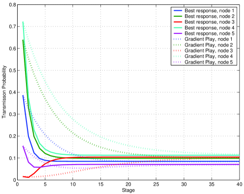
Figure 6: Dynamics of Algorithms 1 and 2.

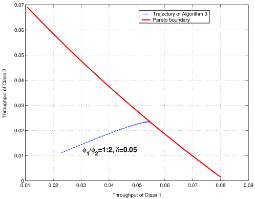
Figure 7: The trajectory of Algorithm 3.

We first illustrate the evolution of transmission probabilities of Algorithm 1 and 2. We simulate a single-cell network of 5 nodes. For each node, the initial transmission probability $p_{k}^{0}$ is uniformly distributed in $[0,1]$ and $a_{k}$ is uniformly distributed between 5 and 10. The stepsize in the gradient play is $\gamma=0.02$. Fig. 6 compares the trajectory of the transmission probability updates in both Algorithm 1 and 2 in a single realization, under the assumption that node $k$ can perfectly estimate the probability $\prod_{j\in\mathcal{K}\backslash\{k\}}(1-p_{j})$, $\forall k\in\mathcal{K}$. The best response update converges in around 8 iterations and the gradient play experiences a more smooth trajectory and the same equilibrium is attained after 35 iterations. In addition, to illustrate how individual nodes can adaptively adjust their algorithm parameters and improve their throughput, we simulate a scenario with two traffic classes. Each traffic class consists of 5 nodes and the initial algorithm parameters of class 1 and 2 are $\phi_{1}=30$ and $\phi_{2}=60$, respectively. The discount factor in Algorithm 3 is $\delta=0.05$. The blue dotted curve in Fig. 7 indicates that the operating point moves towards the red Pareto boundary until the outer loop detects that the desired efficiency is reached.

In practice, packet transmission over wireless links, e.g. IEEE 802.11 WLANs, involves extra protocol overheads, such as inter-frame space and packet header. Assuming these realistic communication scenarios, we compare various performance metrics, including throughput, fairness, convergence, and stability, between our proposed conjecture-based algorithms, the P-MAC protocol in [32], and the IEEE 802.11 DCF. To evaluate these metrics, the physical layer parameters need to be specified. In the simulation, we assume that each wireless device operates at the IEEE 802.11a PHY mode-8, and the key parameters are summarized in Table I. We assume no transmission errors and the RTS/CTS mechanism is disabled. The aggregate network throughput can be calculated using Bianchi’s model [35]

$$\mathcal{T}=\frac{P_{s}L_{d}}{(1-P_{tr})T_{slot}+P_{s}T_{s}+P_{tr}T_{c}-P_{s}T_{c}},$$ (56)

where $P_{s}=\sum_{n=1}^{N}|\mathcal{F}_{n}|\cdot p_{n}\cdot(1-p_{n})^{|\mathcal{F}_{n}|-1}\cdot\prod_{m\neq n}(1-p_{m})^{|\mathcal{F}_{n}|}$ is the probability that a transmission occurring on the channel is successful, $P_{tr}=1-\prod_{n=1}^{N}(1-p_{n})^{|\mathcal{F}_{n}|}$ is the probability that at least one transmission attempt happens, $T_{s}$ is the average time of a successful transmission, and $T_{c}$ is the average duration of a collision. The detailed derivation of $T_{s}$ and $T_{c}$ using the given network parameters in Table I can be found in [32][35]. The parameters in P-MAC are set according to [32]. The contention window sizes in the IEEE 802.11 DCF are $CW_{min}=16$ and $CW_{max}=1024$. In Algorithm 3, individual nodes monitor the aggregate throughput to determine whether to adjust the parameter $a_{k}$. The numerical results are obtained using a MAC simulation program in [35]. Our comparison results are summarized as follows.

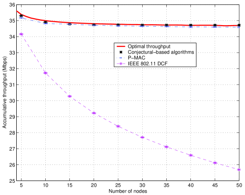
Figure 8: Comparison of the accumulative throughput in the IEEE 802.11 DCF, P-MAC, and conjecture-based algorithms. Error bars correspond to the standard deviation of the mean of the 100 measurements sampled at each point. The error bars in the remaining figures are as in this figure.

First, the throughput of the three algorithms is compared. We vary the total number of nodes $K$ from 4 to 50, in which $\lceil K/2\rceil$ nodes carry class-1 traffic and the remaining nodes carry class-2 traffic. The positive weights of class-1 and class-2 are $\chi_{1}=1$ and $\chi_{2}=0.5$. The initial parameters in Algorithm 3 are chosen to be $\phi_{1}=3K/\chi_{1}$ and $\phi_{2}=3K/\chi_{2}$. As shown in Fig. 8, both the conjecture-based algorithm and P-MAC significantly outperform the IEEE 802.11 DCF. The IEEE 802.11 DCF achieves the lowest throughput, because the lack of adaptation mechanism of the contention window size causes more frequent packet collisions as the number of nodes increases. Surprisingly, the performance of the conjectural equilibrium attained by Algorithm 3 achieves the maximum achievable throughput. It also outperforms P-MAC, because P-MAC uses approximation to derive closed-form expressions for the transmission probabilities of different traffic class.

Next, we evaluate the short-term fairness of different protocols using the quantitative fairness index introduced in [32]

$$\textbf{F}=\frac{\mu(\mathcal{T}_{k}/\chi_{n})}{\mu(\mathcal{T}_{k}/\chi_{n})+\sigma(\mathcal{T}_{k}/\chi_{n})},k\in\mathcal{F}_{n}$$ (57)

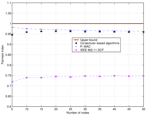
Figure 9: Comparison of the achieved fairness of the IEEE 802.11 DCF, P-MAC, and Algorithm 3.

in which $\mathcal{T}_{k}$ denote the throughput of node $k$ that belongs to traffic class $n$, and $\mu$ and $\sigma$ are, respectively, the mean and the standard deviation of $\mathcal{T}_{n}/\chi_{n}$ over all the active data traffic flows. We simulate a transmission duration of 3 minutes. The stage duration in Algorithm 3 is set as 50 successful transmissions. As shown in Fig. 9, we can see that Algorithm 3 and P-MAC are comparable in their fairness performance and the achieved fairness index is always above 0.95 regardless of the network configuration. On the other hand, the fairness performance of 802.11 DCF is much poorer than the previous two algorithms because the DCF protocol provides no fairness guarantee.

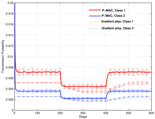
Figure 10: The dynamics of the transmission probabilities in P-MAC and Algorithm 3.

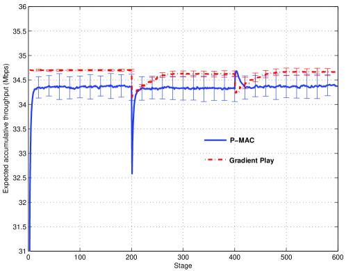
Figure 11: The dynamics of the accumulative throughput in P-MAC and Algorithm 3.

Last, in order to compare the convergence and the stability of different protocols for time-varying traffic, we simulate a network in which the number of active nodes fluctuates over time. In order to cope with traffic fluctuation, we slightly modify the outer loop in Algorithm 3. Once some nodes join or leave the network (this can be detected either by tracking the contention signal $\prod_{k\in\mathcal{K}}(1-p_{k})$ or estimating the total number of nodes in the network [36]), the adaptation of $a_{k}$ is activated. Specifically, if more nodes join the network, $a_{k}\leftarrow a_{k}(1+\delta)$, otherwise, $a_{k}\leftarrow a_{k}(1-\delta)$. At the beginning, $|\mathcal{F}_{1}|=|\mathcal{F}_{2}|=25$. At stage 200, 15 class-1 and 15 class-2 nodes join the network. These nodes leave the network at the 400th stage. The algorithm parameter $a_{k}$ is updated every 5 stages and the stepsize in the gradient play is $\gamma=0.003$. Fig. 10 and Fig. 11 show the variation of the transmission probabilities for both traffic classes and the expected accumulative throughput over time. P-MAC does not converge due to the lack of feedback control, which agrees with the observation about the instability of P-MAC reported in [13]. In addition, the optimal transmission probabilities computed by P-MAC and the conjecture-based algorithms are different under the same network parameters because of the approximation used in P-MAC. As shown in Fig. 10, nodes deploying P-MAC transmit with a higher probabilities than the conjecture-based algorithms, which creates a more congested environment. As a result, the accumulative throughput achieved by P-MAC is slightly lower than the optimal throughput. In contrast, the conjecture-based algorithms enable the nodes adaptively tune their parameters $a_{k}$ to maximize the network throughput while maintaining the weighted fairness as well as the system stability. As shown in Fig. 10 and Fig. 11, during stage [200,300] and [400,470], both the best response and the gradient play autonomously adapt their parameter $a_{k}$ until it converges to the optimal operating point. As discussed before, the best response learning converges faster than the gradient play learning. To give a quantitative measure of the stability, the standard deviations of the expected accumulative throughput in Fig. 11 for different algorithms satisfy $\sigma(\mathcal{T}_{P-MAC}^{Expected})/\sigma(\mathcal{T}_{BIO}^{Expected})\approx 7$ and the actual achieved accumulative throughput satisfy $\sigma(\mathcal{T}_{P-MAC}^{Actual})/\sigma(\mathcal{T}_{BIO}^{Actual})\approx 2$. We can see that, thanks to the inherent feedback control mechanism, both bio-inspired learning algorithm exhibit superior stability performance than P-MAC.

We also simulate the evolution trajectory of the transmission probabilities of the proposed Algorithm 1 and the algorithm in [16]. Both algorithms are essentially the best-response based algorithms. Specifically, we consider a network with $K=6$. The peak data rates for different nodes are $r_{1}=6$, $r_{2}=36$, $r_{3}=9$, $r_{4}=12$, $r_{5}=18$, and $r_{6}=54$, all in Mbps. We apply the algorithm in [16] to solve the following network utility maximization problem:

$$\max_{\textbf{p}\in P}\sum_{k\in\mathcal{K}}\frac{1}{1-\alpha}\bigl{[}r_{k}p_{k}\prod_{j\in\mathcal{K}\backslash\{k\}}(1-p_{j})\bigr{]}^{1-\alpha},$$ (58)

in which $\alpha=2$. The optimal solution corresponds to the belief configuration $a_{1}=2.03,a_{2}=3.93,a_{3}=2.32,a_{4}=2.55,a_{5}=2.97$, and $a_{6}=4.74$. The trajectory of both algorithms are shown in Fig. 12. We can see that, both algorithms converge very fast and oscillate around the neighborhood to the optimal solution after several iterations. However, as we discussed before, the algorithm in [16] requires individual nodes to decode all the received packet headers and estimate the transmission probabilities of the other nodes individually, which introduces a great internal computational overhead when the network size grows large. In contrast, nodes deploying Algorithm 1 only have to estimate the probability of having a free channel without the need of decoding all the packets, which substantially reduces their computational efforts.

We simulate the performance of the proposed algorithms in an ad-hoc network contained in a $100m\times 100m$ square area. Nodes in the square area are placed in the random manner. Two nodes can interfere with each other if their distance is no more than $40m$, i.e. $D_{th}=40m$. We simulate three scenarios with the node numbers $K=\{10,20,40\}$. The Pareto-efficient point that we select is the associated operating point with the link weighted vector $\omega_{k}=1,1\leq k\leq K/2,\textrm{and}\ 0.5,K/2<k\leq K$ in (53). We can see from Fig. 13 that, $\rho(\textbf{J}^{BR})\leq 1$ holds for all the simulated topologies. As shown in Fig. 13, in some realizations, $\rho(\textbf{J}^{BR})=1$, and hence, the associate operating points are not asymptotically stable. This will occur when two nodes interfere with each other and they do not interfere and are not interfered by the remaining nodes in the entire ad-hoc network. On the other hand, the stability improves as the number of nodes increases. As long as the density of nodes is sufficiently large, the stability of the conjecture-based algorithm on the Pareto-efficient operating point can be achieved. Fig. 14 and Fig. 15 show the evolution of transmission probabilities and accumulative throughput for the IEEE 802.11 DCF and Algorithm 1 in a 10-node ad-hoc network with a randomly generated topology. The trajectory of the IEEE 802.11 DCF is obtained using the model in [12]. The parameter $a_{k}$ in Algorithm 1 is chosen to be $|O_{k}|$. The intuition behind is that, if $|O_{k}|=0$, node $k$ can transmit at the maximal probability without interfering with any node. On the other hand, if $|O_{k}|$ is large, node $k$ should backoff adequately such that the reciprocity can be established. As shown in the figures, Algorithm 1 converges faster and achieves higher throughput than DCF. Similar results have been observed in the other simulated topologies.

VI Conclusion

In this paper, we propose distributed learning solutions that enable autonomous nodes to improve their throughput performance in random access networks. It is well-known that whenever biological entities behave selfishly and myopically, a tragedy of commons might take place, which has also been observed in the context of random access control. Hence, we investigate whether forming internal belief functions and learning the impact of various actions can alter the interaction outcome among these intelligent nodes. Specifically, two bio-inspired learning mechanisms are proposed to dynamically update individual nodes’ transmission probabilities. It is analytically proven that the entire throughput region essentially consist of stable conjectural equilibria. In addition, we prove that the conjecture-based approach achieves the weighted fairness for heterogeneous traffic classes and extend the distributed learning solutions to ad-hoc networks. Simulation results have shown that the proposed algorithms achieve significant performance improvement against existing protocols, including the IEEE 802.11 DCF and the P-MAC protocol, in terms of not only fairness and throughput but also convergence and stability. A potential future direction is to investigate how to detect and prevent misbehavior for these bio-inspired solutions.

TABLE I: IEEE 802.11a PHY mode-8 parameters

Parameters	Value
Duration of an Idle Slot ($T_{slot}$)	9 $\mu s$
Duration of PHY Header ($T_{PHY}$)	20 $\mu s$
SIFS Time ($T_{SIFS}$)	16 $\mu s$
DIFS Time ($T_{DIFS}$)	34 $\mu s$
Propagation Delay ($T_{d}$)	1 $\mu s$
MAC Header ($L_{MAC}$)	28 octets
Packet Payload Size ($L_{d}$)	2304 octets
ACK Frame Size ($L_{ACK}$)	14 octets
Data Rate ($R_{t}$)	54 Mbps

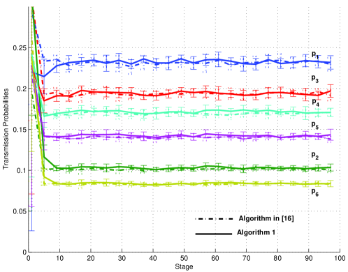
Figure 12: Comparison between Algorithm 1 and the algorithm in [16].

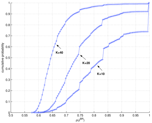
Figure 13: Cumulative distribution function of $\rho(\textbf{J}^{BR})$ in ad-hoc networks.

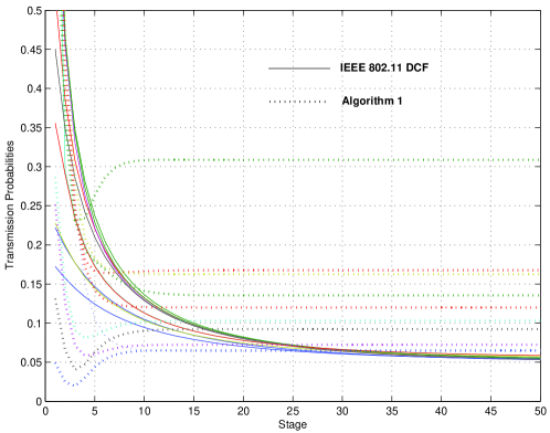
Figure 14: Transmission probabilities of Algorithm 1 and the IEEE 802.11 DCF in ad-hoc networks.

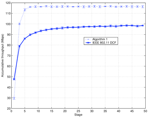
Figure 15: Accumulative throughput of Algorithm 1 and the IEEE 802.11 DCF in ad-hoc networks.

References

- [1] S. Haykin, “Cognitive Radio: Brain-empowered wireless communications”, IEEE J. Selected Areas in Commu., vol. 23, pp. 201-220, 2005.
- [2] F. Dressler and I. Carreras, Advances in Biologically Inspired Information Systems - Models, Methods, and Tools, Studies in Computational Intelligence (SCI), vol. 69, Berlin, Heidelberg, New York, Springer, 2007.
- [3] T. Suda, T. Itao, and M Matsuo, “The Bio-Networking Architecture: The Biologically Inspired Approach to the Design of Scalable, Adaptive, and Survivable/Available Network Applications,” in The Internet as a Large-Scale Complex System, the Santafe Institute Book Series, Oxford University Press, 2005.
- [4] R. Dawkins, The Selfish Gene, 2nd ed., United Kingdom: Oxford University Press, 1989.
- [5] J. M. Smith, Evolution and the Theory of Games, Cambridge: Cambridge University Press, 1982.
- [6] D. Fudenberg and D. Levine, The Theory of Learning in Games, Cambridge, MA: MIT Press, 1999.
- [7] M. Nowak, “Five Rules for the Evolution of Cooperation,” Science, vol. 314, pp. 1560-1563, 2006.
- [8] E. Friedman and S. Shenker. “Learning and Implementation on the Internet”, Manuscript. New Brunswick: Rutgers University, Department of Economics, 1997. (available at http://citeseer.ist.psu.edu/eric98learning.html)
- [9] C. Long, Q. Zhang, B. Li, H. Yang, and X. Guan, “Non-Cooperative Power Control for Wireless Ad Hoc Networks with Repeated Games”, IEEE J. Select. Areas Commun., vol. 25, pp. 1101-1112, Aug, 2007.
- [10] F. Fu and M. van der Schaar,“Learning to Compete for Resources in Wireless Stochastic Games”, IEEE Trans. Veh. Tech., to appear.
- [11] Y. Jin and G. Kesidis, “Equilibria of a noncooperative game for heterogeneous users of an Aloha networks”, IEEE Commun. Lett., vol. 6, no. 7, pp. 282-284, July 2002.
- [12] J. Lee, A. Tang, J. Huang, M. Chiang, and A. R. Calderbank, “Reverse-engineering MAC: A non-cooperative game model”, IEEE J. Select. Areas Commun., vol. 25, no. 6, pp. 1135-1147, Aug. 2007.
- [13] T. Cui, L. Chen, and S. H. Low, “A Game-Theoretic Framework for Medium Access Control”, IEEE J. Select. Areas Commun., vol. 26, no. 7, pp. 1116-1127, Sep. 2008.
- [14] Čagalj, S. Ganeriwal, I. Aad, and J. P. Hubaux, “On selfish behavior in CSMA/CA networks”, in Proc. IEEE Infocom, pp. 2513-2524, Mar. 2005.
- [15] J. Lee, M. Chiang, and R. A. Calderbank, “Utility-optimal random-access control”, IEEE Trans. Wireless Commun., vol. 6, no. 7, pp. 2741-2751, July 2007.
- [16] A. Mohsenian-Rad, J. Huang, M. Chiang, and V. Wong, “Utility-Optimal Random Access: Optimal Performance Without Frequent Explicit Message Passing”, IEEE Trans. on Wireless Commu., vol. 8, no. 2, 898-911, Feb. 2009.
- [17] R. T. B. Ma, V. Misra, and D. Rubenstein, “An Analysis of Generalized Slotted-Aloha Protocols”, IEEE/ACM Trans. Networking, accepted for future publication.
- [18] M. P. Wellman and J. Hu, “Conjectural equilibrium in multiagent learning,” Machine Learning, vol. 33, pp. 179-200, 1998.
- [19] C. Figuières, A. Jean-Marie, N. Quérou, and M. Tidball, Theory of Conjectural Variations, World Scientific Publishing, 2004.
- [20] S. G. Massaquoi, “Modeling the function of the cerebellum in scheduled linear servo control of simple horizontal planar arm movements,” Ph.D. dissertation, MIT, Cambridge, MA, 1999.
- [21] S. Jo, “A neurobiological model of the recovery strategies from perturbed walking,” BioSystems, vol. 90, no. 3, pp. 750-768, 2007.
- [22] U. Dieckmann and R. Law, “The dynamical theory of coevolution: a derivation from stochastic ecological processes”, Journal of Mathematical Biology, vol. 34, pp. 579-612, 1996.
- [23] P. Taylor and T. Day, “Evolutionary stability under the replicator and the gradient dynamics”, Evolutionary Ecology, vol. 11, pp. 579-590, 1997.
- [24] L. Edelstein-Keshet, Mathematical Models in Biology, Random House, New York, 1988.
- [25] A. Jean-Marie and M. Tidball, “Adapting behaviors through a learning process”, Journal of Economic Behavior and Organization, vol. 60, pp. 399-422, 2006.
- [26] R. Myerson, Game Theory, Harvard University Press, 1991.
- [27] R. A. Horn and C. R. Johnson, Matrix Analysis, Cambridge, U.K. : Cambridge Univ. Press, 1991.
- [28] A. Granas and J. Dugundji, Fixed Point Theory, New York: Springer-Verlag, 2003.
- [29] D. Chiu and R. Jain, “Analysis of the Increase/Decrease Algorithms for Congestion Avoidance in Computer Networks”, Journal of Computer Networks and ISDN, vol. 17, no. 1, pp. 1-14, June 1989.
- [30] J. Massey and P. Mathys, “The collision channel without feedback”, IEEE Trans. Inform. Theory, vol. 31, no. 2, pp. 192-204, 1985.
- [31] D. P. Bertsekas and J. N. Tsitsiklis, Parallel and Distributed Computation. Englewood Cliffs, New Jersey: Prentice Hall, 1997.
- [32] D. Qiao and K. G. Shin, “Achieving efficient channel utilization and weighted fairness for data communications in IEEE 802.11 WLAN under the DCF”, Proc. IWQoS 2002, pp. 227-236, May 2002.
- [33] P. Gupta and A. L. Stolyar, “Optimal Throughput Allocation in General Random-Access Networks”, Proc. CISS 2006, pp. 1254-1259, Mar. 2006.
- [34] IEEE 802.11a, Part 11: Wireless LAN Medium Access Control (MAC) and Physical Layer (PHY) specifications: High-speed Physical Layer in the 5 GHz Band, Supplement to IEEE 802.11 Standard, Sep. 1999.
- [35] G. Bianchi, “Performance Analysis of the IEEE 802.11 Distributed Coordination Function,” IEEE J. Selected Areas in Commu., vol. 18, no. 3, pp. 535-547, Mar. 2000.
- [36] G. Bianchi and I. Tinnirello, “Kalman Filter Estimation of the Number of Competing Terminals in an IEEE 802.11 Network,” Proc. of IEEE Infocom, 2003.
- [37] T. Nandagopal, T. E. Kim, X. Gao and V. Bharghhavan, “Achieving MAC layer fairness in wireless packet networks,” Proc. ACM Mobicom, 2000.
- [38] K. J. Astrom and T. Hagglund, PID Controllers: Theory, design and tuning. Instrument society of America, 2nd edition, 1995.
- [39] J. S. Simonoff, Smoothing Methods in Statistics, Springer Series in Statistics. Springer-Verlag New York, 1996.