Quantum Hall resistances of multiterminal top-gated graphene device

Abstract

Four-terminal resistances, both longitudinal and diagonal, of a locally gated graphene device are measured in the quantum-Hall (QH) regime. In sharp distinction from previous two-terminal studies [J. R. Williams et al., Science 317, 638 (2007); B. Özyilmaz et al., Phys. Rev. Lett. 99, 166804 (2007)], asymmetric QH resistances are observed, which provide information on reflection as well as transmission of the QH edge states. Most quantized values of resistances are well analyzed by the assumption that all edge states are equally populated. Contrary to the expectation, however, a 5/2 transmission of the edge states is also found, which may be caused by incomplete mode mixing and/or by the presence of counter-propagating edge states. This four-terminal scheme can be conveniently used to study the edge-state equilibration in locally gated graphene devices as well as mono- and multi-layer graphene hybrid structures.

I INTRODUCTION

Landau-level splitting in two-dimensional (2D) electron systems under a perpendicular magnetic field reveals the well-known quantum-Hall (QH) effect. Klitzing80 ; Beenakker91 When the Fermi energy is set between two Landau levels, a current circulates along the edge conduction states in a (chiral) direction determined by the carrier type and the direction of the magnetic field. Halperin82 ; Buttiker88 ; Beenakker91 Utilizing this chiral character of the edge states one can devise diverse solid-state beam splitters out of 2D electron gas systems. Oliver99 ; Henny99 ; Ji03

On the other hand, due to the relativistic nature of the carriers, graphene, a 2D honeycomb lattice of carbon atoms, shows the half-integer QH effect. Novoselov04 ; Novoselov05 ; Zhang05 ; Neto09 Thus, the manipulation of the edge states in graphene can be of particular interest. However, the electrostatic deflection of the edge state Beenakker91 ; Oliver99 ; Henny99 ; Ji03 is not realizable in graphene due to the Klein tunneling of the carriers through an electrostatic barrier. Katsnelson06 Nonetheless, the possibility of controlling the edge-state transmission in graphene has been confirmed by locally modulating the filling factor $\nu$ and the chiral direction of the edge states. Ozyilmaz07 ; Williams07 Two-terminal observation of the edge-state transmission in graphene to date is well explained by the complete-mode-mixing hypothesis where all edge states are equally populated at p-n interfaces. Ozyilmaz07 ; Williams07 ; Abanin07 QH plateaus in two-terminal measurements, however, can be distorted depending on the sample geometry and the contact inhomogeneities. Abanin08 ; Williams08 Moreover, the two-terminal conductance gives the information only on the edge-state transmission, lacking the information on the reflection. Thus, for the better manipulation of the edge states of an arbitrary-shaped graphene device, one needs geometry-independent measurements that can furnish information on both the edge-state reflection and transmission.

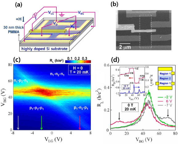
Figure 1: (Color) (a) Schematic measurement configuration. (b) Scanning electron microscope image of the device after depositing a local gate, the brightest central part. The broken lines represent the graphene edges and the boundary of the PMMA insulation layer is evident by the contrast change near the top of the image. The white scale bar represents 2 $\mu$m. (c) Two-dimensional color map of $R_{L}$($V_{LG}$,$V_{BG}$) for 0 T at 20 mK. A set of carrier types in the regions 1 and 2 is labeled in each quadrant. (d) $V_{BG}$ dependence of $R_{L}$ at $V_{LG}$=-2 V, 6 V and -7 V extracted from (c) as indicated by arrows with the same color (green, red, and gray, respectively). Left inset: the $R_{D}$ (upper) and $R_{L}$ (lower) as a function of $V_{BG}$ at $V_{LG}$= -2 V and 10 T, showing the half-integer QH effect. Right inset: a schematic top view of the device, where the local gate is placed on top of the colored region at the center (the region 2).

In this paper, we report on four-terminal QH transport measurements in a top-gated bi-polar graphene device, which show the quantization of longitudinal QH resistances as well as an asymmetry in the diagonal QH resistances (the meaning will be defined below). Our measurement scheme provides precise information on the reflected QH edge states in addition to the transmitted ones as can be obtained from two-terminal measurements. Ozyilmaz07 ; Williams07 Most of the results are in good quantitative agreement with the Landauer-Büttiker formula, Beenakker91 ; Buttiker88 while unexpected resistance plateaus corresponding to the 5/2 transmission of edge state are also observed. It may arise from the incomplete mode mixing and/or unusual QH edge states that are possibly present under the local gate. Chklovskii92 ; Rossier07 ; Silvestrov08 ; Zhang06 ; Abanin07-1 ; Jiang07 ; Abanin07-2 This simple four-terminal scheme will allow an additional insight into the edge-state equilibration in bipolar graphene systems. Results of this study can also be utilized for the spatial manipulation of the Dirac fermions in graphene, which is one of the hot issues in graphene studies.

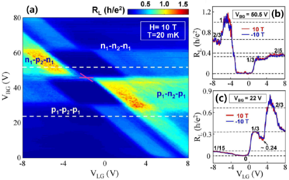
Figure 2: (Color) (a) Two-dimensional plot of $R_{L}$($V_{LG}$,$V_{BG}$) for 10 T at 20 mK. A set of carrier types in the regions 1 and 2 is labeled in each quadrant. (b,c) Plots of $R_{L}$($V_{LG}$) extracted from (a) at $V_{BG}$=50.5 V and 22 V, as indicated by the white broken lines in (a). Broken lines represent the calculation result based on the Landauer-Büttiker formula.

II SAMPLE PREPARATION and VERIFICATION

The sample was prepared by mechanically exfoliating monolayer graphene Novoselov04 on a silicon substrate covered with a 300-nm-thick oxide layer where the silicon substrate was used as a back gate (BG). Electrical contacts of Cr (5 nm)/Au (20 nm) were patterned by the method described elsewhere. Ki08 It was then followed by spin-coating a 30-nm-thick polymethyl methacrylate (PMMA, 950 K, 2% in anisole) dielectric layer on top of the device, which was cross-linked by high doses (15000 $\mu$C/cm²) of electron beams Huard07 with 20 keV. Finally, a local gate (LG) of Cr (5 nm)/Au (40 nm) was deposited at the center of the device [Fig. 1(b)]. The device was cooled down to 20 mK in a dilution fridge (Oxford Instruments, Model AST). The longitudinal ($R_{L}$=$V_{L}$/$I$) and diagonal ($R_{D}$=$V_{D}$/$I$) resistances were measured simultaneously with two lock-in amplifiers, synchronized with each other at $I$=2 nA and $f$=13.3 Hz [see Fig. 1(a)].

Figure 1(c) shows a 2D color map of $R_{L}$($V_{LG}$,$V_{BG}$) measured at zero magnetic field in units of $h$/$e^{2}$ (all resistances will be presented in this unit afterward). In the figure, horizontal and diagonal bands crossing at ($V_{LG}$,$V_{BG}$)$\approx$(-2 V,46 V) are identified, which divide the map into four different quadrants. These bands represent positions of local resistance maxima arising from the change in the carriers in the region underneath the local gate (the region 2) with respect to the outside region (the region 1) [the right inset of Fig. 1(d)]. Figure 1(d) is the one-dimensional slice plot of $R_{L}$($V_{BG}$) that is extracted from Fig. 1(c) at $V_{LG}$=-2 V, 6 V, and -7 V. It indicates that the position of the secondary resistance peak, corresponding to the diagonal pattern in Fig. 1(c), directly depends on $V_{LG}$ while that of the dominant resistance peak, the horizontal pattern in Fig. 1(c), is almost insensitive to $V_{LG}$. This leads to a conclusion that the horizontal (diagonal) band is from the charge-neutrality point in the region 1 (in the region 2) where the carrier type is altered. It verifies the successful performance of our bipolar device. Ozyilmaz07 ; Williams07 ; Huard07 ; Gorbachev08 ; Stander09 Additionally, in the left inset of Fig. 1(d), we show the half-integer QH effect, $R_{D}$ (upper) and $R_{L}$ (lower), taken at $V_{LG}$=-2 V and $B$=10 T, indicating that our device consists of a monolayer graphene sheet. Novoselov05 ; Zhang05 ; Neto09

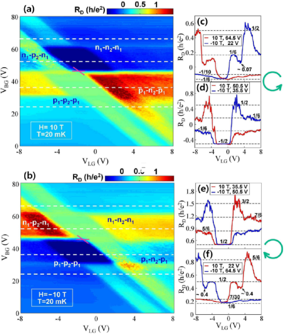
Figure 3: (Color) [(a) and (b)] Two-dimensional plots of $R_{D}$($V_{LG}$,$V_{BG}$) at 10 T and -10 T, respectively. A set of carrier types in the regions 1 and 2 is labeled in each quadrant. [(c)-(f)] Red curves: $R_{D}$($V_{LG}$) extracted from (a) at $V_{BG}$=64.5 V, 50.5 V, 35.5 V, and 22 V. Blue curves: $R_{D}$($V_{LG}$) extracted from (b) at $V_{BG}$=22 V, 35.5 V, 50.5 V, and 64.5 V. Thus, (c) and (d) correspond to the counterclockwise edge state in the region 1, while (e) and (f) to the clockwise edge state in the same region as denoted on the right. The extraction $V_{BG}$ values are marked by the white broken lines in (a) and (b). Broken lines represent the calculation results from the Landauer-Büttiker formula.

III EXPERIMENTAL RESULTS

The 2D color map of $R_{L}$($V_{LG}$,$V_{BG}$) measured at 10 T is shown in Fig. 2(a). It displays several skewed blocks of different resistances, implying the quantization of the longitudinal resistance. Details are more clearly seen in one-dimensional slices, $R_{L}$($V_{LG}$), of Fig. 2(a) for fixed values of $V_{BG}$. In Figs. 2(b) and 2(c), $R_{L}$($V_{LG}$) is displayed for $V_{BG}$=50.5 V and 22 V, respectively. The red and blue curves were taken at 10 T and -10 T, respectively. Two curves almost completely overlap with each other. Dominant resistance plateaus exist at zero resistance in the region -3 V$<$$V_{LG}$$<$1 V [Fig. 2(b)] and -3 V$<$$V_{LG}$$<$0 V [Fig. 2(c)], which arise from the full transmission of the edge states when the filling factors in the regions 1 ($\nu_{1}$) and 2 ($\nu_{2}$) are identical. In addition to these trivial ones, one also finds plateaus of non-zero fractional resistances such as 1/15, 1/3, and 2/3 in a certain range of $V_{LG}$. This quantization directly demonstrates that a portion of the edge states is reflected at the interfaces between the regions 1 and 2 for non-identical filling factors $\nu_{1}$ and $\nu_{2}$, which is consistent with the previous two-terminal conductance measurements. Ozyilmaz07 ; Williams07 The quantized values of $R_{L}$ are in excellent agreement with the calculation results following Ref. [4] as represented by the broken lines in Figs. 2(b) and 2(c), the details of which will be discussed below.

Now, let us focus on the diagonal resistance $R_{D}$, which exhibits far richer features. As seen in Figs. 3(a) and 3(b), the 2D plots of $R_{D}$($V_{LG}$,$V_{BG}$) taken at 10 T and -10 T, respectively, also reveal skewed blocks of different resistances, but with overall features much different from Fig. 2(a). First of all, both Figs. 3(a) and 3(b) show no inversion symmetry with respect to the crossing point at $V_{BG}$$\sim$46 V and $V_{LG}$$\sim$-2 V, where $\nu_{1}$=$\nu_{2}$=0 (the zero point). Nonetheless, there exists an inversion symmetry between Figs. 3(a) and 3(b), or equivalently a 180^∘ rotational symmetry between them with respect to the zero point, which is in sharp distinction from the feature of $R_{L}$ [Fig. 2(a)] as well as the previous two-terminal results. Ozyilmaz07 ; Williams07 More details are revealed by the one-dimensional slices shown in Figs. 3(c)-3(f), which are again extracted from Fig. 3(a) for 10 T (red curves) and Fig. 3(b) for -10 T (blue curves). The corresponding values of $V_{BG}$ are specified in each figure. The figures illustrate that the data taken at 10 T and -10 T are mirror symmetric with respect to $V_{LG}$$\sim$-1 V, which again confirms the inversion symmetry of $R_{D}$ between the two opposite field directions.

Figures 3(e) and 3(f) show the $R_{D}$ measured when carriers in the region 1 are holes ($\nu_{1}$$<$0) for 10 T and electrons ($\nu_{1}$$>$0) for -10 T, which corresponds to the clockwise edge-states in the region 1. Most of the quantized resistances in these figures match with the inverse of two-terminal conductance observed previously. Ozyilmaz07 Thus, $R_{D}$ in this region corresponds to the two-terminal (or Hall) resistance of transmitted edge states. In contrast to the two-terminal results, however, Figs. 3(e) and (f) show clear 1/2 plateaus. This indicates that the disorder effect, which has been regarded as the cause of the observed reduction in the conductance for $\nu_{1}$=$\nu_{2}$=$\pm$2 in the previous study, Ozyilmaz07 is negligible in this four-terminal measurement. On the other hand, in Figs. 3(c) and 3(d) (for $\nu_{1}$$>$0 at 10 T and $\nu_{1}$$<$0 at -10 T), $\pm$1/2, $\pm$1/6, and -1/10 plateaus are seen together with a sign change at certain values of $V_{LG}$. This sign change seems to be odd because these plateaus correspond to the counterclockwise edge states in the region 1, where $R_{D}$ is supposed to be negative. A careful analysis, however, indicates that the $R_{D}$ for $\nu_{1}$$\cdot$$\nu_{2}$$<$0 [the n₁-p₂-n₁ region in Fig. 3(a) and the p₁-n₂-p₁ region in Fig. 3(b)] is nothing but the Hall resistance for the clockwise edge states in the region 2, which should be positive as observed. But, still counterintuitive positive (1/6) plateaus appear in Fig. 3(c) even for the counterclockwise edge states both in the regions 1 and 2 [$\nu_{1}$$\cdot$$\nu_{2}$$>$0 for the n₁-n₂-n₁ region in Fig. 3(a) and for the p₁-p₂-p₁ region in Fig. 3(b)]. This can be accounted for in terms of the Landauer-Büttiker formalism for the edge states as will be shown below. Beenakker91 ; Buttiker88

IV DISCUSSION

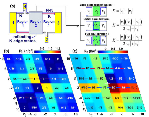
Figure 4: (Color) (a) Schematic top view of the edge-state configuration. Electrical contacts are shown in yellow and thick arrows represent the chiral direction of QH edge states. The case of the clockwise circulation in region 1 is shown as an example. We assume that $K$ out of $N$ edge states are reflected at the interfaces between the regions 1 and 2 (blue arrows). On the right, three possible equilibration processes in a graphene p-n-p device and corresponding values of $K$ for each regime are illustrated. [(b) and (c)] Two-dimensional plot of the calculated $R_{L}$ and $R_{D}$ for a positive magnetic field as a function of $\nu_{1}$ and $\nu_{2}$. In both figures, calculated values of the resistance plateaus are written at the center of each block in units of $h$/$e^{2}$. Horizontal lines represent the filling factor $\nu_{1}$ where one-dimensional data in Figs. 2 and 3 are extracted.

The Landauer-Büttiker formula Beenakker91 ; Buttiker88 is suitable for studying the one-dimensional edge-state transport where the current through the lead $\alpha$ ($I_{\alpha}$) is expressed as a linear combination of transmission coefficients ($T_{\alpha\beta}$) multiplied by the corresponding chemical potentials ($\mu_{\beta}$). Accordingly, it is required to evaluate the scattering matrix ($\widehat{S}$) with the elements $T_{\alpha\beta}$’s and then solve the linear equations ($\overrightarrow{I}$=$\widehat{S}$$\overrightarrow{\mu}$), which is straightforward in our case because the reflection ($K$) happens at p-n interfaces only [see Fig. 4(a)]. This procedure is adopted to obtain $R_{L}$ and $R_{D}$ in Ref. [4] for the configuration that is identical to ours. It is suggested that $R_{L}$ is finite unless $K$ is zero and $R_{D}$ has two different values ($R_{D}^{+}$ and $R_{D}^{-}$), depending on the measurement configurations.

$$R_{1342} \rightarrow \frac{h}{e^{2}}\frac{1}{N-K}\equiv R_{D}^{+},$$

$$R_{4213} \rightarrow -\frac{h}{e^{2}}\frac{N-2K}{N(N-K)}=R_{D}^{+}-\frac{h}{e^{2}}\frac{2}{N}\equiv R_{D}^{-},$$ (1)

$$R_{1243} = R_{4312}\rightarrow\frac{h}{e^{2}}\frac{K}{N(N-K)}=R_{D}^{+}-\frac{h}{e^{2}}\frac{1}{N}\equiv R_{L},$$

where $R_{\alpha\beta\gamma\delta}$ represents the resistance measured between the voltage leads $\gamma$ and $\delta$ for the current injection from leads $\alpha$ to $\beta$. In Eq. (IV) it is assumed that $N$ edge states circulate in the clockwise direction in the region 1, i.e., $\nu_{1}$$<$0 ($>$0) for 10 T (-10 T) in our case. For a direct comparison with the theoretical expectation, Buttiker88 we adopt a four-terminal schematic sample configuration in Fig. 4(a) rather than a five-terminal one corresponding to the actual device. Since each resistance ($R_{L}$ or $R_{D}$) was obtained in a four-terminal configuration, the schematic is equivalent to the real device configuration, namely, $R_{D}$ ($R_{L}$) in Fig. 1(a) corresponds to $R_{1342}$ ($R_{4312}$) in Fig. 4(a). Since $R_{1342}$ and $R_{4213}$ depend on the chiral direction of incoming edge states $R_{D}$ corresponds to $R_{D}^{+}$ ($R_{D}^{-}$) for the clockwise (counterclockwise) edge states in the region 1. Thus, $R_{D}$ changes as the sign of $\nu_{1}$ changes at a fixed magnetic-field direction, but it represents the same resistance if both $\nu_{1}$ and the magnetic-field direction are altered. This explains the inversion symmetry shown in Fig. 3.

Two-terminal resistance in a bipolar configuration studied previously Ozyilmaz07 corresponds to $R_{D}^{+}$ only in Eq. (IV), which is the Hall resistance from the $N-K$ transmitted edge states. It is consistent with our observation shown in Figs. 3(e) and 3(f), which correspond to the clockwise edge states in the region 1. But, the information on the reflected edge states is lost in the two-terminal process. On the other hand, $R_{D}^{-}$ represents the eliminated Hall resistance by the $K$ reflected edge-states, which can be observed only in a four-terminal configuration. This implies that the average of $R_{D}^{+}$ and $R_{D}^{-}$, ($R_{D}^{+}$$-$$R_{D}^{-}$)/2, provides the Hall resistance of $N$ incoming edge states (the sign for $R_{D}^{-}$ is reversed because $R_{D}^{+}$ and $R_{D}^{-}$ are measured in the opposite direction with respect to the current flow). Thus, if more than a half of the incoming edge states are reflected (2$K$$>$$N$), $R_{D}^{-}$ can change the sign, accounting for the odd sign of resistances seen in Figs. 3(c) and 3(d). On the other hand, $R_{L}$ indicates the difference between the (two-terminal) Hall resistance of the $N-K$ transmitted and the $N$ incoming edge states which is always positive or equal to zero for $K$=0. In consequence, all the unexpected features in $R_{D}$ as well as the finite value of $R_{L}$ are well accounted for at least qualitatively.

For a quantitative analysis, we estimated the number of the reflected edge states ($K$) in three different regimes: Ozyilmaz07 the edge-state-transmission regime ($\nu_{1}$$\cdot$$\nu_{2}$$>$0, $N$=$|\nu_{1}|$$\geq$$|\nu_{2}|$), partial-equilibration regime ($\nu_{1}$$\cdot$$\nu_{2}$$>$0, $N$=$|\nu_{1}|$$<$$|\nu_{2}|$), and full-equilibration regime ($\nu_{1}$$\cdot$$\nu_{2}$$<$0, $N$=$|\nu_{1}|$). Based on the complete-mode-mixing hypothesis, Ozyilmaz07 ; Abanin07 it is evident that $K$ is equal to $|\nu_{1}|$-$|\nu_{2}|$ in the edge-state-transmission regime, where the extra edge states in the region 1 ($|\nu_{1}|$-$|\nu_{2}|$) are forbidden in the region 2. In the partial-equilibration regime, the excess states ($|\nu_{2}|$-$|\nu_{1}|$) circulate in the region 2 while in partial equilibration with the incoming edge states ($|\nu_{1}|$). Finally, in the full-equilibration regime, the edge states in the regions 1 ($|\nu_{1}|$) and 2 ($|\nu_{2}|$) circulate in opposite directions, propagating in the same direction along the p-n interfaces and equilibrate with each other. In the last two regimes, one can calculate $K$ by using the current-conservation relation. Ozyilmaz07 Schematic edge-state circulation and values of the $K$ are illustrated in the right panel of Fig. 4(a) for each regime. With these values of filling factor in Eq. (IV), the $R_{L}$ and $R_{D}$ are calculated as functions of $\nu_{1}$ and $\nu_{2}$ as shown below.

(a) Edge-state transmission regime:

$$R_{D} = \begin{cases}\frac{h}{e^{2}}\frac{1}{|\nu_{2}|}&\text{($\nu_{1}$$<$0 at 10 T or $\nu_{1}$$>$0 at -10 T)}\\ -\frac{h}{e^{2}}\frac{2|\nu_{2}|-|\nu_{1}|}{|\nu_{1}||\nu_{2}|}&\text{($\nu_{1}$$>$0 at 10 T or $\nu_{1}$$<$0 at -10 T)}\end{cases},$$

$$R_{L} = \frac{h}{e^{2}}\frac{|\nu_{1}|-|\nu_{2}|}{|\nu_{1}||\nu_{2}|}$$ (2)

(b) Partial equilibration regime:

$$R_{D} = \begin{cases}\frac{h}{e^{2}}\frac{2|\nu_{2}|-|\nu_{1}|}{|\nu_{1}||\nu_{2}|}&\text{($\nu_{1}$$<$0 at 10 T or $\nu_{1}$$>$0 at -10 T)}\\ -\frac{h}{e^{2}}\frac{1}{|\nu_{2}|}&\text{($\nu_{1}$$>$0 at 10 T or $\nu_{1}$$<$0 at -10 T)}\end{cases},$$

$$R_{L} = \frac{h}{e^{2}}\frac{|\nu_{2}|-|\nu_{1}|}{|\nu_{1}||\nu_{2}|}$$ (3)

(c) Full equilibration regime:

$$R_{D} = \begin{cases}\frac{h}{e^{2}}\frac{2|\nu_{2}|+|\nu_{1}|}{|\nu_{1}||\nu_{2}|}&\text{($\nu_{1}$$<$0 at 10 T or $\nu_{1}$$>$0 at -10 T)}\\ \frac{h}{e^{2}}\frac{1}{|\nu_{2}|}&\text{($\nu_{1}$$>$0 at 10 T or $\nu_{1}$$<$0 at -10 T)}\end{cases},$$

$$R_{L} = \frac{h}{e^{2}}\frac{|\nu_{1}|+|\nu_{2}|}{|\nu_{1}||\nu_{2}|}$$ (4)

Results for a positive magnetic field (10 T) are summarized in two color maps in Figs. 4(b) and 4(c), respectively, with the calculated resistance labeled in each block. As seen in Fig. 4(b), unless $\nu_{1}$=$\nu_{2}$, $R_{L}$ becomes positive and is in good quantitative agreement with the observed results as denoted by the broken lines in Figs. 2(b) and 2(c). The values of $R_{D}$ are also well reproduced by the calculation as shown in Fig. 4(c) as well as Fig. 3(a). Although not shown, the observed -10 T data of $R_{D}$ [Fig. 3(b)] are also well fit by the calculation. Furthermore, for $\nu_{1}$$>$0 ($<$0) at 10 T (-10 T), the calculated $R_{D}$ becomes positive in the region where $\nu_{1}$$\cdot$$\nu_{2}$$<$0 or $|\nu_{1}|$$>$2$|\nu_{2}|$ and $\nu_{1}$$\cdot$$\nu_{2}$$>$0, reproducing the odd sign of resistances found in Figs. 3(c) and 3(d). Again, all the observed features of $R_{D}$ are well accounted for in terms of the Landauer-Büttiker formula. Beenakker91 ; Buttiker88 Since all of these results are linked to the chiral-directional dependence of $R_{D}$, one can conclude that edge states in graphene also behave in the same way as those in a conventional 2D electron gas, Beenakker91 although the QH effect itself is distinct by the Dirac nature of charge carriers. Novoselov05 ; Zhang05 ; Neto09

V 5/2 TRANSMISSION of EDGE STATES

Most of the observed results in the color maps shown in Figs. 2 and 3 are quantitatively accounted for. However, one can distinguish some additional features which appear as a faint diagonal bands crossing from the bottom-right region to the top-left region of the figures in the ranges $V_{BG}$$>$$\sim$60 V and $V_{BG}$$<$$\sim$30 V near the boundary where $\nu_{2}$ changes sign. In fact, these band structures constitute additional resistance plateaus of $\sim$0.24, $\sim$0.07, and $\sim$0.4 as indicated by arrows in Figs. 2(c), 3(c), and 3(f), respectively. Solving Eq. (IV) for $R_{L}$$\sim$0.24, $R_{D}^{-}$$\sim$0.07, and $R_{D}^{+}$$\sim$0.4 at $N$=$|\nu_{1}|$=6 gives almost identical $K$ values as $\sim$3.54, $\sim$3.52, and $\sim$3.5, respectively. This indicates that these unexpected resistance plateaus are all produced by a single 5/2 (=$N$$-$$K$=6$-$7/2) edge-state transmission for $|\nu_{1}|$=6, $|\nu_{2}|$=2, and $\nu_{1}$$\cdot$$\nu_{2}$$>$0, just before $\nu_{2}$ changes sign or, equivalently, just before the edge-state transmission regime turns into the full equilibration regime. This state may be related to the disorder in the region 2, but no related features are present at $\nu_{1}$=$\nu_{2}$=$\pm$2 in our measurement. Ozyilmaz07 In addition, the disorder effect is not supposed to be significant in our four-terminal measurement.

Another possible explanation is based on the fact that the plateaus take place near the boundary between the edge-state transmission and the full-equilibration regimes. One may imagine the presence of counter-propagating edge states: for instance, $|2|$+$|\varepsilon|$ clockwise edge states and $|\varepsilon|$ counterclockwise edge states in the region 2. Here, we expect that $|\varepsilon|$ should be an integer less than 2, because no fractional QH effect is present Hou07 ; Chamon08 and the maximum filling factor in the region 2 is two. However, a simple calculation of the total reflection $K$ by adding two different $K$ values for the clockwise edge states (edge-state transmission) and the counterclockwise ones (full equilibration) leads to $|\varepsilon|$ much larger than 2 (about 4.7, corresponding to $K$=7/2), which is far from the expectation.

The discrepancy can arise from the incomplete mode mixing for the counter-propagating edge states, which leads to the 5/2 transmission when only two and a half out of three clockwise edge states participate in the equilibration process completely. These counter-propagating edge states may originate from the compressible and incompressible edge states Chklovskii92 ; Rossier07 ; Silvestrov08 formed near the boundary of the graphene by the charge accumulation as suggested for the graphene sheet placed above a global backgate. Rossier07 ; Silvestrov08 However, the strange diagonal bands observed in our study indicate that the local gate, by some means, further enhances the charge accumulation. The presence of the QH ferromagnet states Zhang06 ; Abanin07-1 ; Jiang07 ; Abanin07-2 can also be considered for the counter-propagating edge states. But, the Zeeman energy in 10 T is only about 20 K, Abanin07-2 which is much smaller than the energy difference between the lowest and the first exited Landau levels, $\sim$700 K. Novoselov07 Although this phenomenon can be understood by assuming both the incomplete mode mixing and the presence of counter-propagating edge states, Chklovskii92 ; Rossier07 ; Silvestrov08 ; Zhang06 ; Abanin07-1 ; Jiang07 ; Abanin07-2 further theoretical and experimental investigation is required for a conclusive account for the effect.

VI SUMMARY

We studied the edge-state equilibration processes in a locally gated p-n-p junction of the graphene by measuring the four-terminal QH resistances. Our scheme enables measurements of finite longitudinal and asymmetric diagonal QH resistances, which furnish precise information on the reflected as well as the transmitted QH edge states. Most of our observations are quantitatively analyzed by the Landauer-Büttiker formula Beenakker91 ; Buttiker88 based on the complete-mode mixing hypothesis. But, unexpected resistance plateaus corresponding to the 5/2 transmission of edge states are also observed. We suggest that it may arise from the incomplete mode mixing and/or the presence of the counter-propagating QH edge states. Chklovskii92 ; Rossier07 ; Silvestrov08 ; Zhang06 ; Abanin07-1 ; Jiang07 ; Abanin07-2

Our simple four-terminal measurement scheme reported here is not sensitive to the contact resistance and the sample geometry, so that it can be conveniently used for the edge-state manipulation of arbitrary-shaped devices such as Mach-Zehnder interferometers. Ji03 Moreover, with the additional information on the reflection of the edge states, this scheme enables one to investigate the details of the edge-state equilibration at p-n interfaces such as 5/2 transmission of the edge states found in this study. It can be also employed to investigate the edge states in hybrid structures of mono-layer and multi-layer graphene. Nilsson07 ; Puls08

- (1) K. v. Klitzing, G. Dorda, and M. Pepper, Phys. Rev. Lett. 45, 494 (1980).
- (2) See a review in C. W. J. Beenakker and H. van Houten, Solid State Phys. 44, 1 (1991); also found in arXiv:0412664v1.
- (3) B. I. Halperin, Phys. Rev. B 25, 2185 (1982).
- (4) M. Büttiker, Phys. Rev. B 38, 9375 (1988).
- (5) M. Henny, S. Oberholzer, C. Strunk, T. Heinzel, K. Ensslin, M. Holland, and C. Schönenberger, Science 284, 296 (1999).
- (6) W. D. Oliver, J. Kim, R. C. Liu, and Y. Yamamoto, Science 284, 299 (1999).
- (7) Y. Ji, Y. Chung, D. Sprinzak, M. Heiblum, D. Mahalu, and H. Shtrikman, Nature (London) 422, 415 (2003).
- (8) K. S. Novoselov, A. K. Geim, S. V. Morozov, D. Jiang, Y. Zhang, S. V. Dubonos, I. V. Grigorieva, and A. A. Firsov, Science 306, 666 (2004).
- (9) K. S. Novoselov, A. K. Geim, S. V. Morozov, D. Jiang, M. I. Katsnelson, I. V. Grigorieva, S. V. Dubonos, and A. A. Firsov, Nature (London) 438, 197 (2005).
- (10) Y. Zhang, Y. W. Tan, H. L. Stormer, and P. Kim, Nature (London) 438, 201 (2005).
- (11) For the recent review, see A. H. Castro Neto, F. Guinea, N. M. R. Peres, K. S. Novoselov, and A. K. Geim, Rev. Mod. Phys. 81, 109 (2009).
- (12) M. I. Katsnelson, K. S. Novoselov, and A. K. Geim, Nat. Phys. 2, 620 (2006).
- (13) B. Özyilmaz, P. Jarillo-Herrero, D. Efetov, D. A. Abanin, L. S. Levitov, and P. Kim, Phys. Rev. Lett. 99, 166804 (2007).
- (14) J. R. Williams, L. DiCarlo, and C. M. Marcus, Science 317, 638 (2007).
- (15) D. A. Abanin and L. S. Levitov, Science 317, 641 (2007).
- (16) D. A. Abanin and L. S. Levitov, Phys. Rev. B 78, 035416 (2008).
- (17) J. R. Williams, D. A. Abanin, L. DiCarlo, L. S. Levitov, and C. M. Marcus, arXiv:0810.3397 (unpublished).
- (18) D. B. Chklovskii, B. I. Shklovskii, and L. I. Glazman, Phys. Rev. B 46, 4026 (1992).
- (19) J. Fernandez-Rossier, J. J. Palacios, and L. Brey, Phys. Rev. B 75, 205441 (2007).
- (20) P. G. Silvestrov and K. B. Efetov, Phys. Rev. B 77, 155436 (2008).
- (21) Y. Zhang, Z. Jiang, J. P. Small, M. S. Purewal, Y. W. Tan, M. Fazlollahi, J. D. Chudow, J. A. Jaszczak, H. L. Stormer, and P. Kim, Phys. Rev. Lett. 96, 136806 (2006).
- (22) D. A. Abanin, K. S. Novoselov, U. Zeitler, P. A. Lee, A. K. Geim, and L. S. Levitov, Phys. Rev. Lett. 98, 196806 (2007).
- (23) Z. Jiang, Y. Zhang, H. L. Stormer, and P. Kim, Phys. Rev. Lett. 99, 106802 (2007).
- (24) D. A. Abanin, P. A. Lee, and L. S. Levitov, Solid State Commun. 143, 77 (2007).
- (25) D. K. Ki, D. Jeong, J. H. Choi, H. J. Lee, and K. S. Park, Phys. Rev. B 78, 125409 (2008).
- (26) B. Huard, J. A. Sulpizio, N. Stander, K. Todd, B. Yang, and D. Goldhaber-Gordon, Phys. Rev. Lett. 98, 236803 (2007).
- (27) N. Stander, B. Huard, and D. Goldhaber-Gordon, Phys. Rev. Lett. 102, 026807 (2009).
- (28) R. V. Gorbachev, A. S. Mayorov, A. K. Savchenko, D. W. Horsell, and F. Guinea, Nano. Lett. 8, 1995 (2008).
- (29) C. Y. Hou, C. Chamon, and C. Mudry, Phys. Rev. Lett. 98, 186809 (2007).
- (30) C. Chamon, C. Y. Hou, R. Jackiw, C. Mudry, S. Y. Pi, and G. Semenoff, Phys. Rev. B 77, 235431 (2008).
- (31) K. S. Novoselov, Z. Jiang, Y. Zhang, S. V. Morozov, H. L. Stormer, U. Zeitler, J. C. Maan, G. S. Boebinger, P. Kim, and A. K. Geim, Science 315, 1379 (2007).
- (32) C. P. Puls, N. E. Staley, and Y. Liu, arXiv:0809.1392 (unpublished).
- (33) J. Nilsson, A. H. Castro Neto, F. Guinea, and N. M. R. Peres, Phys. Rev. B 76, 165416 (2007).