Dynamics and evolution of an eruptive flare

Abstract

Aims. We study the dynamics and the evolution of a C2.3 two-ribbon flare, developed on 2002 August 11, during the impulsive phase as well as during the long gradual phase. To this end we obtained multiwavelength observations using the CDS spectrometer aboard SOHO, facilities at the National Solar Observatory/Sacramento Peak, and the TRACE and RHESSI spacecrafts.

Methods. CDS spectroheliograms in the Fe xix, Fe xvi, O v and He i lines allows us to determine the velocity field at different heights/temperatures during the flare and to compare them with the chromospheric velocity fields deduced from H$\alpha$ image differences. TRACE images in the 17.1 nm band greatly help in determining the morphology and the evolution of the flaring structures.

Results. During the impulsive phase a strong blue-shifted Fe xix component ($-200$ km s^-1) is observed at the footpoints of the flaring loop system, together with a red-shifted emission of O v and He i lines ($20$ km s^-1). In one footpoint simultaneous H$\alpha$ data are also available and we find, at the same time and location, downflows with an inferred velocity between 4 and 10 km s^-1. We also verify that the “instantaneous” momenta of the oppositely directed flows detected in Fe xix and H$\alpha$ are equal within one order of magnitude. These signatures are in general agreement with the scenario of explosive chromospheric evaporation. Combining RHESSI and CDS data after the coronal upflows have ceased, we prove that, independently from the filling factor, an essential contribution to the density of the post-flare loop system is supplied from evaporated chromospheric material. Finally, we consider the cooling of this loop system, that becomes successively visible in progressively colder signatures during the gradual phase. We show that the observed cooling behaviour can be obtained assuming a coronal filling factor of $\approx$ 0.2 to 0.5.

1 Introduction

Most solar flare models are based on the idea that flares arise from the sudden release of free magnetic energy stored in the corona in non-potential configurations (e.g., Klimchuk et al., 1988). The bulk of the energy is released through reconnection of the magnetic field lines in the corona (Petschek, 1964; Kopp & Pneuman, 1976; Shibata, 1996) and then transported down to the chromosphere along the magnetic field lines by accelerated particles or by a thermal conduction front. Hydrodynamic simulations indicate that both non-thermal electrons (Fisher et al., 1985a, b; Mariska et al., 1989) and a thermal conduction front (Gan et al., 1991) should lead to the evaporation of chromospheric material. Models by Fisher et al. (1985a) result in upflows (gentle evaporation) or downflows (explosive evaporation), on both transition-region (TR) and chromosphere, depending on the energy flux of the impinging electrons, with downflows predicted for large energy fluxes. In the case of explosive evaporation the overpressure of evaporated plasma drives upward motions in the corona and downward motions in the chromosphere and it is expected that the momenta of the oppositely moving plasma should be balanced. The chromospheric evaporation injects mass into the corona to fill coronal loops that appear as the soft X-ray (SXR) flare and that eventually cool down radiatively and/or conductively forming cold H$\alpha$ post-flare loops (see, e.g., Moore et al., 1980). Although this general picture seems well established, the details of some of the key processes assumed to take place remain to be verified. The small temporal and spatial scales involved, together with the need for comprehensive temporal and height coverage, conjure up to make “complete” flare observations a very demanding task.

Blue-shifts of lines formed at flare temperatures during the impulsive phase (corresponding to upflow velocities in excess of several hundreds kilometre per second) have been observed since the early 1980s (e.g., Doschek et al., 1980; Antonucci et al., 1982) and confirmed with the Bragg Crystal Spectrometer aboard Yohkoh (BCS, Culhane et al., 1991). However, the majority of these observations revealed only a blue asymmetry, indicating the presence of a large, static component even in the early phases of the flare (e.g., Bentley et al., 1994; Gan & Watanabe, 1997), rather than wholly blue-shifted profiles as predicted by hydrodynamic models (e.g., Emslie et al., 1992; Gan et al., 1995). To which extent the lack of spatial resolution might have influenced these observations is not easily quantifiable (neither BCS nor earlier spectrometers provided any effective spatial resolution on the solar surface). Since reconnection is expected to occur at very small spatial scales, it might well be that the associated chromospheric evaporation takes place in rather confined portions of the solar surface. This is indeed the case in eruptive flares, for which, at any given time, the evaporation in the reconnection scenario occurs in a very thin shell ($\leq$ 1^′′) located on the outer part of the flaring loop system (Forbes & Acton, 1996; Falchi et al., 1997), and the heating of individual field lines is supposed to last only 100 s or so (Forbes, 2003). The smearing introduced by observing over the whole disk would then significantly alter the relevant signals. Hydrodynamic simulations modelling solar flare emission with multiple loops (Hori et al., 1998; Warren & Doschek, 2005) have shown that it is possible to reproduce the line profiles dominated by the stationary component (as observed by BCS) with a simple model based on the successive independent heating of small scale threads. Only the simulated line profiles for individual threads do show strongly blue shifted line profiles.

Spatially and temporally resolved observations of flare lines have finally become available with the advent of the Coronal Diagnostic Spectrometer (CDS, Harrison et al., 1995) aboard SOHO, which provides stigmatic slit images in the 31 to 38 nm (NIS-1) and 51 to 63 nm (NIS-2) range with a spatial resolution of few seconds of arc and a cadence depending upon the adopted observing program. Various authors have since reported the presence of blueshifted emission in hot coronal lines during flares, signalling upflows of up to $\approx 200$ km s^-1 (Czaykowska et al., 1999; Del Zanna et al., 2002; Brosius, 2003; Teriaca et al., 2003; Brosius & Phillips, 2004), but the total number of events analysed up to now remains small. Moreover, the same authors report about intricate patterns of blue- and red-shifted emission in TR lines, depending both on the location within the flaring region and the phase of the flare, that still need to be consistently explained within the theory of chromospheric evaporation. Finally, spatially and temporally resolved observations of flare lines need to be combined with simultaneous chromospheric observations, in order to verify the spatial and temporal coincidence of chromospheric downflows with hot plasma upflows. In fact, while many authors have reported on the simultaneous appearance of redshifts in chromospheric lines and blue-shifts in flare lines during the early phase of flares (e.g., Canfield et al., 1990b; Falchi et al., 1992; Wülser et al., 1994), to date the only direct proof that such shifts arise from spatially coincident areas has been provided by Teriaca et al. (2003). However, due to the observational setup, their coronal and chromospheric data were not simultaneous, leading to the need of further observations.

In this context, we report here on comprehensive, multi-instrument observations of a small eruptive flare, covering its temporal evolution from the impulsive phase and related evaporation throughout the gradual phase and appearance of cold postflare loops. Spatially resolved CDS spectra allow us to study the dynamics of the upper atmosphere at various times during the flare, while simultaneous chromospheric observations provide a test for the chromospheric evaporation scenario. RHESSI data acquired during the gradual phase, combined with CDS measurements, provide a final element in support of the chromospheric evaporation. Other SOHO instruments and TRACE, provide various context information and help us in defining and constraining the flare evolution.

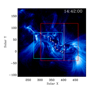
Figure 1: TRACE image (logarithmic scale) in the 17.1 nm band showing AR 10061 at flare peak. The dark grey (red in the electronic version) box indicates the UBF FOV while the area rastered by CDS/NIS is represented by the light grey (blue) box. The white vertical line marks the position of the DST spectrograph slit. Here and in the following images, the white dashed line shows the apparent magnetic inversion line obtained from MDI data in the region around the filament.

2 Observations and data analysis

The observations were acquired during a coordinated campaign between ground based and SOHO instruments aimed at studying flare events by sampling the solar atmosphere from the chromosphere to the corona. The main instruments involved were the CDS/NIS spectrometer aboard SOHO and facilities at the NSO/Sacramento Peak. The analysed flare developed at about 14:40 UTC in region NOAA 10061 on 2002 August 11 (N10W20). Although small (GOES class C2.3), the flare was clearly eruptive in character with an impulsive rise and a long decay phase, and developed two ribbons visible at various wavelengths on opposite sides of the magnetic neutral line. A second flare, not studied here, developed in the same region around 16:25 UTC.

2.1 Data

Ground-based data – Monochromatic images at several wavelengths have been acquired, with a temporal cadence of a few seconds, by the tunable Universal Birefringent Filter (UBF: H$\alpha$ line centre, $-60$ pm, $+60$ pm and $-150$ pm off centre; He i D3; Na i D2 and in the continuum) and by the Zeiss filter (H$\alpha$ $+150$ pm) at the Dunn Solar Telescope of the National Solar Observatory (DST/NSO). The field of view (FOV) was of about $150^{\prime\prime}\times 150^{\prime\prime}$ with a spatial scale of $0.5^{\prime\prime}\times 0.5^{\prime\prime}$. Spectra have been acquired with the Horizontal Spectrograph (HSG) in three chromospheric lines (Ca ii K, H$\gamma$ and He i D3) with a temporal cadence of 4 s and the fixed slit positioned as indicated in Fig. 1.

Space-born data – Spectroheliograms of a $120^{\prime\prime}\times 110^{\prime\prime}$ area (mostly overlapping the UBF FOV, see Fig. 1) were obtained with the Normal Incidence Spectrometer (NIS) of the CDS experiment (Harrison et al., 1995) starting at 14:26:27 UTC. Each raster was obtained in $\approx 210$ s by stepping the $4^{\prime\prime}$ wide slit eastward in 19 steps of $6^{\prime\prime}$. On board binning over two rows yielded a pixel size of 3.4^′′ along the slit. Spectra were acquired in the He i 58.43 nm ($2\times 10^{4}$ K), O v 62.97 nm ($2.5\times 10^{5}$ K), Fe xvi 36.08 nm ($2\times 10^{6}$ K) and Fe xix 59.22 nm ($8\times 10^{6}$ K) lines. Every ten rasters an additional step of $\approx 5^{\prime\prime}$ westward was performed to compensate for the solar rotation. During the entire period of CDS observations AR 10061 was constantly monitored by the Transition Region and Coronal Explorer (TRACE, Handy et al., 1999) that provided images in the 17.1 nm band (Fe ix – x, $\approx 10^{6}$ K) with a spatial scale of $1^{\prime\prime}$ pixel^-1 (on board $2\times 2$ binning) and a cadence of $\approx 7.5$ s. The Reuven Ramaty High-Energy Solar Spectroscopic Imager (RHESSI, Lin et al., 2002) exited its night a few minutes after the peak phase of the flare, and provided information on hot ($\approx 10^{7}$ K) thermal flare plasma as well as on non-thermal components. From RHESSI data in the energy band 3 to 10 keV, we derived images with spatial resolution up to $2^{\prime\prime}$ and spectra of the spatially integrated flux with 1 keV spectral resolution. Unfortunately, due to particle precipitation events, only three different times could be analysed during the gradual phase of the flare. Finally, MDI (Scherrer et al., 1995) full-disk magnetograms taken at 14:27:34 UTC and 16:03:34 UTC were used to determine the position of the photospheric apparent magnetic inversion line.

2.2 Data co-alignment

Data from the different instruments were aligned using MDI continuum data as a reference. UBF continuum images (and, hence, all DST data) were easily aligned first. Afterwards, CDS images in the He i 58.4 nm line were aligned with the UBF images acquired in H$\alpha$ line centre. Moreover, the flare kernels at the loop footpoints in the TRACE 17.1 nm images appear strikingly similar to those observed in H$\alpha$ line centre, allowing a very good relative alignment. The brightening of the flare kernels is also very clear in the CDS O v images, providing further constraints. We estimate the alignment between TRACE, MDI and ground data to be precise within $1^{\prime\prime}$ and within $2^{\prime\prime}$ with CDS. RHESSI images are more difficult to align and the precision is estimated around $5^{\prime\prime}$. Each spectrum or image has been tagged with its precise acquisition time so that light and velocity curves obtained using data from different instruments can be properly computed.

2.3 Measurement of line-of-sight motions

Ground-based data – Strong flows in the flaring chromosphere are often measured through spectral line asymmetries, defined generally with the bisector (Zarro et al., 1988; Falchi et al., 1992). In the portion of the flare ribbon intersected by the HSG slit, the Ca ii K line shows indeed an emission core with a red asymmetry. The H$\gamma$ line, instead, remains in absorption (with a central radiance higher than in the reference quiet area), so that several blends in its wings prevent a reliable measure of the otherwise visible asymmetry. The He i D3 line is only barely visible. The velocity component along the line of sight (LOS) for the HSG spectra was hence computed using the bisector of the emission core of the Ca ii K line, in all 16 pixels in the ribbon area and for 41 different times. Unfortunately, the (fixed) spectrograph slit was positioned slightly outside the FOV covered by the CDS rasters (see Fig. 1), so that no direct comparison of velocities deduced from HSG spectra can be performed. However, in the area of the flaring ribbons within the CDS FOV, we could use the H$\alpha$ images acquired at several wavelengths to estimate the chromospheric velocities. To this end, difference images at $\pm$60 pm and $\pm$150 pm were computed. In all flaring kernels the differences between the red and blue wings of H$\alpha$ were positive and very close in value, while the radiances in both the centre and in the wings remained higher than in the reference quiet area. This implies an asymmetric H$\alpha$ profile with a stronger emission in the red part of the line and hence a downward velocity for all flaring kernels. To estimate the value of this velocity, we calibrated the radiance differences obtained from the H$\alpha$ images in the kernel where HSG spectra have been acquired with the velocities obtained from the Ca ii K spectra. This was done for all times and pixels for which a reliable estimate of the Ca ii K velocity was available (about 500 points). We find that the average H$\alpha$ radiance difference observed in the flare kernels, both at $\Delta\lambda\pm 60$ pm and $\Delta\lambda\pm 150$ pm, corresponds to a downward velocity between 4 and 10 km s^-1. Similar velocity values have been found from H$\alpha$ line profiles in the case of small (GOES class B – C) flares (e.g., Schmieder et al., 1998).

CDS spectra – Spectra acquired after recovery of the SOHO spacecraft are characterised by broad and asymmetric line profiles that were fitted with an opportune template provided within the CDS software. The template consists of a Gaussian component (with all parameters free to vary) and a wing (non-Gaussian) component whose parameters are established for both NIS-1 and NIS-2 spectra.

The analysis of line positions reveals that no trends (either parallel or perpendicular to the slit direction) are present within a single raster. However, the analysis of the raster-averaged NIS-2 line positions versus time reveal a small linear trend that is equal in He i and O v. The shift amounts to $\approx$ 20 km s^-1 over two hours. This trend has been accounted for by providing a corrected (shifted) wavelength vector for each NIS-2 line in each raster. No such a trend is visible in the Fe xvi NIS-1 line.

Flows in the He i 58.43 nm, O v 62.97 nm, and Fe xvi 36.08 nm lines have been measured fitting a single component to the line profiles. These lines have an obvious pre-flare component, so that a reference wavelength has been obtained averaging the central positions derived from the fitting for the whole dataset. Velocities have then been computed simply using the Doppler-shift of the flare profiles with respect to the reference wavelength.

The measurement of flows in the hot ($\log\leavevmode\nobreak\ T/$K=6.9) Fe xix 59.22 nm line requires a more careful analysis. The line appears only during flares, so great caution is needed in choosing the reference profile (see discussions in Teriaca et al., 2003; Brosius, 2003). The line profiles obtained averaging all CDS pixels with a radiance greater than 0.16 W m^-2 sr^-1 are identical in width and position in three successive scans during the late phase of the flare (from 14:53:10 to 15:00:10 UTC, times at raster centres), so their average was used as our reference profile. A multi-component fitting was hence applied to the profiles in various pixels and times, constraining the rest component by imposing width and position of the reference profile, while the background (characterised by the Fe xii 59.26 nm line, see Del Zanna & Mason, 2005) was constrained through the average non-flare spectrum.

Figure 2: Soft X-ray full disk flux at 1 UA in the 1 to 8 Å band around the time of the flare (GOES 8 data). The time derivative (dashed line) represents a proxy for the hard X-ray curve (Neupert effect) and shows its maximum around 14:41:20 UTC.

Uncertainties on best-fit parameters are evaluated accounting for data noise (photon statistics, pulse height distribution and readout noise) and the average 3-$\sigma$ uncertainty amounts to 15 to 18 km s^-1 over the active region for single component fitting and to 25 to 30 km s^-1 for double component fitting.

3 Flare evolution

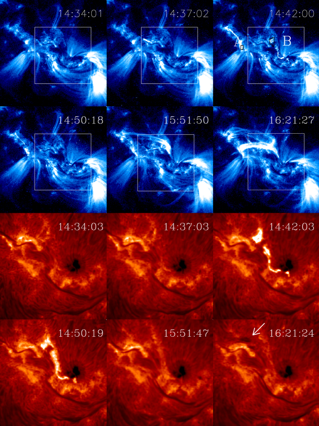
Figure 3: Evolution of the flare: TRACE images (logarithmic scale) in the 17.1 nm band are shown in the first two rows and H$\alpha$ images in the last two rows. The white box in TRACE images indicate the H$\alpha$ FOV. The images at 14:34 UTC show the region just before the flare. The areas (labelled A and B) over which data were integrated to obtain the light and velocity curves shown in Fig. 4 are indicated in black on the TRACE image taken at 14:42:00 UTC. The arrow in the last H$\alpha$ image indicates the cool post-flare loops.

Since RHESSI was in the Earth shadow during the initial phase, no hard X-ray observations were available to define the impulsive phase of the flare. Moreover, the low temporal resolution attained with the CDS rastering mode prevents the use of EUV radiance peaks as a proxy for hard X-ray (HXR) bursts, as was done, e.g., by Brosius (2003). Hence we used the time-derivative of the GOES SXR flux as a proxy for the HXR emission (Neupert effect; Neupert, 1968). Both the 0.1 to 0.8 nm (1.6 to 12.4 keV) flux and its derivative are displayed around the time of the flare development in Figure 2. The main episode of energy release indicated by the Neupert peak is around 14:41:20 UTC, but significant signal is present up to the GOES maximum, i.e., up to around 14:48 UTC. We assume the gradual phase starts after this time.

Figure 3 outlines the main phases of the flare evolution as seen in the TRACE 17.1 nm channel and H$\alpha$ centre. A filament located on the magnetic neutral line is clearly visible in both spectral ranges before the flare. The activation of a portion of this filament is observed around 14:13 UTC in the H$\alpha$ images and lasts up to 14:37 UTC, when it becomes clearly visible also in the TRACE images. The eruption was detected by CDS in the O v line, where upward speeds around 30 km s^-1 were detected at 14:36:33 UTC.

Few minutes later the footpoints of a large loop system (spanning over $6\times 10^{4}$ km on the solar surface) start to brighten, reaching their maximum around 14:42 UTC. The flare ribbons are clearly visible and nearly identical in both TRACE and H$\alpha$ images. Although the east-most ribbon is outside of the FOV of the UBF H$\alpha$ images, we verified its existence in the images acquired by the HASTA telescope (see Fig. 1 in Maltagliati et al., 2006). During the impulsive phase of the flare, the ribbons are associated with large coronal upflows and chromospheric and TR downflows (see next section). The brightenings last several minutes and fade off around 14:50 UTC in the 17.1 nm band while their decay is much longer in H$\alpha$.

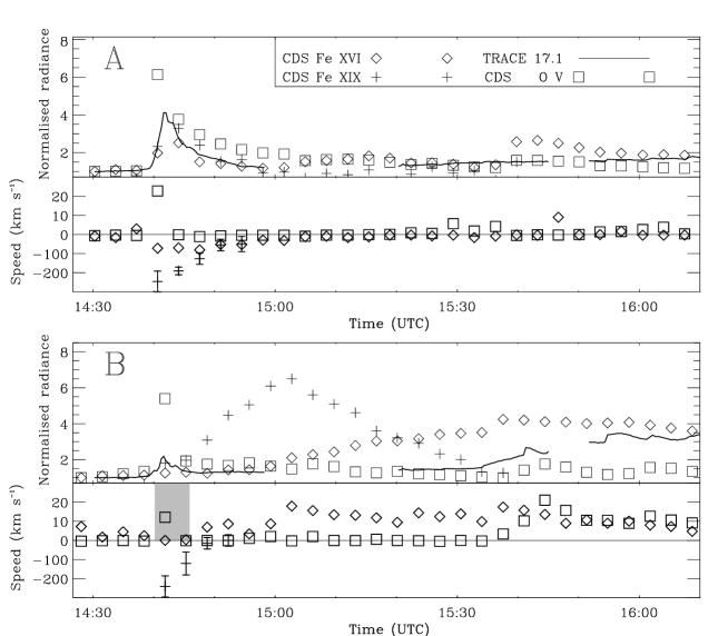
Figure 4: Light and velocity curves at the footpoints (areas A and B in Fig. 3) of the loop system. For clarity reasons uncertainties are only shown for the Fe xix speeds. O v, Fe xvi, and TRACE radiances are normalised to pre-flare values while Fe xix radiances are normalised to the average value reached after the flare (around 15:32 UTC). The average uncertainties in the normalised radiance are of about 0.15. On footpoint A, the average uncertainties in speed are 12 km s^-1 (O v) and 20 km s^-1 (Fe xvi). On footpoint B, the average uncertainties in speed are 9 and 12 km s^-1 for O v and Fe xvi. The shaded area represents the time during which downflows between 4 and 10 km s^-1 were observed in H$\alpha$. (We remind that only for footpoint B we have chromospheric observations). On both panels, the scale of downward (positive) velocities has been expanded for sake of clarity.

Immediately after the GOES maximum, the first RHESSI spectrum (14:50 UTC) between 4 and 10 keV shows a non-thermal component indicating that electron acceleration is still present. During the gradual phase of the flare, two cooling loop systems connecting the ribbons appear in the TRACE images, one around 15:40 UTC, and the other around 16:03 UTC. Fig. 3 shows them at the time of maximum radiance. Finally, these loops appear also as dark features in the H$\alpha$ images at 16:21 UTC, revealing that the plasma has cooled down to temperatures around $10^{4}$ K.

In the following, we will concentrate on the footpoints of the second loop system, contained in the CDS FOV, where most of the brightenings and velocity episodes are visible in our dataset. Figure 4 summarises the radiance and velocity evolution in these footpoints, labelled A and B in Fig. 3 (TRACE image of 14:42:00 UTC). A and B are optimised to obtain a high S/N ratio in the smallest region still showing relevant coronal velocities. The area A consists of three CDS pixels (6$\arcsec\times 10\arcsec$), while the area B, due to the weak emission of the Fe xix line in the westward ribbon, consists of eleven CDS pixels (224 arcsec²).

4 Impulsive phase: chromospheric evaporation

For both footpoints, the radiances of O v and TRACE 17.1 nm undergo a sharp increase and a rapid decay during the impulsive phase. However, Fe xvi and Fe xix present a very different behaviour. In A these hotter signatures increase and decrease rapidly, while in B Fe xvi becomes barely brighter than average and Fe xix begins a slow rise. We believe that these differences reflect the different temperature reached by the evaporated plasma, being hotter in B ($>$10⁷ K, cf. § 5).

4.1 Motions in the flaring ribbons

Footpoint A: Around 14:40 UTC, CDS was scanning the east flaring kernel (A), revealing a strong emission in O v. Both Fe xvi and Fe xix clearly increased their emission with respect to the background. In the 3 pixels defining the kernel A downflows of about $20$ km s^-1 are measured in O v, but adjacent pixels show both strong upflows ($-35$ km s^-1, westward of A) and downflows (60 km s^-1, eastward of A, see Fig. 5). The O v downflows appear clearly associated with the bright kernel visible in TRACE and in the HASTA H$\alpha$ image (see Fig. 1 in Maltagliati et al., 2006). The same velocity pattern is also shown by the He i spectra.

At this time the Fe xix spectrum obtained integrating over A shows a blue-shifted emission with a velocity between $-170$ km s^-1 (single component fitting) and $-250$ km s^-1 (double component fitting, see Fig. 5, top-right). However, given the noise level in the spectrum, it is difficult to establish whether a two component fitting is justified. We thus can assume as a lower limit the value obtained with a single component fit. The same region also shows upward motions around $-70$ km s^-1 in the Fe xvi line. Due to the broad NIS-1 profiles, we have not attempted to separate the strong Fe xvi background component, resulting in a likely underestimate of the upward velocity.

These upward motions of hot plasma seem to originate in the region between the flow patterns of opposite sign observed in TR, but from an area where O v motions are still downward directed ($\approx 20$ km s^-1). Furthermore, if we consider a semi-circular loop with radial legs, the projection effect would amount to about $-2\arcsec$ in the x-direction and thus suggest a link between the upward motions in Fe xix and the even stronger downflows seen in the TR (the target area is on the west hemisphere, the loop direction is east-west, and we assume the Fe xix emission from a region $\approx$5 000 km above that of O v and He i ).

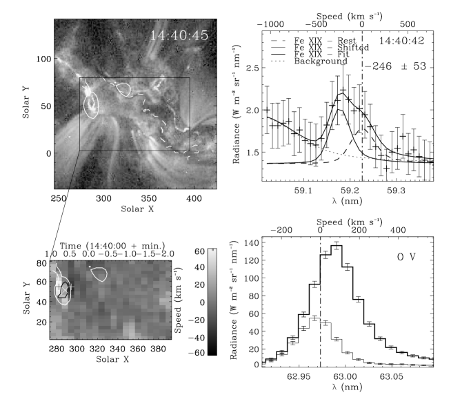
Figure 5: Eastward ribbon (A) at 14:40:45 UTC. The top left panel shows a TRACE image in the 17.1 nm band. The bottom left panel shows a map of the O v LOS velocity within the area encompassed by the black box on the TRACE image. On both panels isocontours of the O v radiances at a level of 5 W m² sr^-1 are shown with white thick lines while the thick black isocontours on the velocity map indicate Fe xix radiances at a level of 90 mW m² sr^-1. The Fe xix profile shown on the top-right panel is obtained by integrating over three pixels along the CDS slit, centred at the location indicated by a white x on the velocity map (area A defined in Fig. 3). The single pixel O v profiles on the bottom right panel refer to the locations indicated by a black + (thick histogram) and a white + (thin histogram) on the velocity map.

Around 14:44 UTC, CDS scanned again this flaring kernel (Fig. 6). The resulting Fe xix profile (bottom panel of the figure) shows a strong blue-shifted component dominating the whole profile. The corresponding velocity is of about $-$200 km s^-1. Upflows of $-70$ km s^-1 are still measured in the coronal Fe xvi. The same velocity pattern seen in O  v and He i during the previous passage is still discernible, with the downflows now weaker ($\approx 20$ km s^-1) and unchanged upflows.

Finally, strong coronal upflows are still visible in the kernel A when CDS scans the area a third time during the impulsive phase, around 14:47:30 UTC ($-170$ km s^-1 with a double component fitting and $-100$ km s^-1 with a single component fitting). O  v and He i do not show any downflow anymore, while the nearby upflow is still present.

Footpoint B: This footpoint is within the DST FOV. Starting from around 14:41 UTC, the difference of H$\alpha$ images obtained at both $\Delta\lambda$=$\pm\leavevmode\nobreak\ 60$ pm and $\pm\leavevmode\nobreak\ 150$ pm shows a red-wing emission excess in correspondence of the flaring kernels, resulting in a downflow velocity of 4 to 10 km s^-1 (cf. § 2.3).

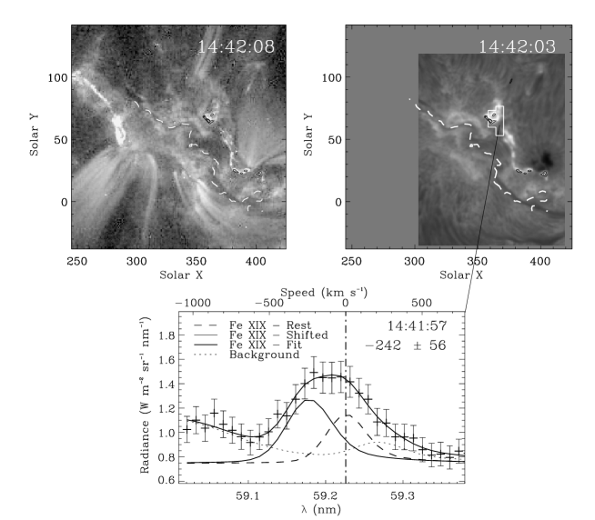
Figure 7: Westward ribbon (B) at 14:42 UTC. Panels are as in Fig. 6. On both images the thin black contours indicate chromospheric downflows of 4 km s^-1 and 7 km s^-1. The Fe xix line profile shown on the bottom panel is obtained by integrating over the area within white solid lines in the H$\alpha$ image (area B defined in Fig. 3). A single component fit (plus background) would result in an upflow speed of ($-125\pm 50$) km s^-1

Around 14:42 UTC this area was rastered over by CDS. Velocities in O v and He i indicate only downwards motions ($\approx$20 km s^-1) outlining the tiny bright features visible at the higher spatial resolution afforded by H$\alpha$ data. Chromospheric downflows are measured at the same time in the same area, and are indicated with thin black contours in the upper panels of Fig.  7. Upflows of more than 200 km s^-1 were measured in Fe xix by averaging over the whole footpoint area. The corresponding profile of the Fe xix line is shown in the bottom panel of the same figure. The fitting procedure reveals a blue-shifted component of the same strength of the stationary component, with a speed of $-$240 km s^-1. A single component fit provides a velocity of about $-$125 km s^-1.

During the next raster at 14:45:23 UTC, CDS still measures strong upward speeds in the Fe xix line (Fig. 4), cospatial and cotemporal with downflows in the low chromosphere (H$\alpha$). The radiance of the blue-shifted component is comparable to that of the stationary component also at this time. At later times, neither the Fe xix nor the H$\alpha$ data show any relevant motions. Hence in this footpoint, the oppositely directed motions measured in low-chromosphere and in hot flare lines, are verified to be co-spatial and co-temporal and to persist for at least 200 s.

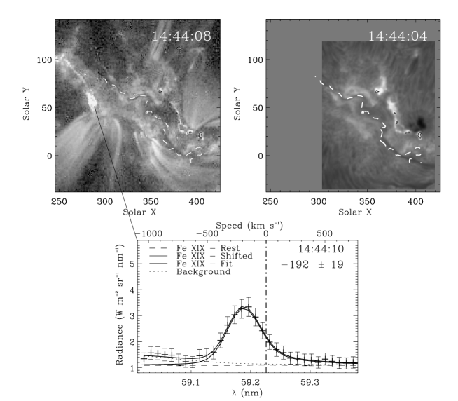
Figure 6: Eastward ribbon (A) at 14:44 UTC. The top left panel shows a TRACE image in the 17.1 nm band while the H$\alpha$ image closest in time is shown on the top right panel. On both images the thin black contours indicate chromospheric downflows of 4 km s^-1. The Fe xix line profile shown on the bottom panel is obtained by integrating over three pixels along the CDS slit (area A defined in Fig. 3).

Contrary to what could be expected, the Fe xvi line does not show any upward velocity within the area B. However, we note that at the times when strong motions are measured in Fe xix, the radiance of the Fe xvi is practically unchanged with respect to its pre-flare values. This also suggests that the evaporated plasma is too hot to generate a shifted component strong enough to be measurable with respect to the Fe xvi background emission.

Comparing the two footpoints, we notice that the Fe xix blue-shifted component is clearly dominating over the stationary one only in the eastward ribbon (A), possibly due to the smaller area used to obtain reliable line profiles. This fact may then support the assumption that multiple thin loops are present in the flaring ribbons at any time, and that they are heated successively, as in the simulations of Warren & Doschek (2005). This is further confirmed by TRACE and H$\alpha$ images that show very clearly the existence of multiple footpoints within the flaring ribbons, brightening at different times. Note also that during the gradual phase (see § 5) post-flare loops of 1$\arcsec$ to 2$\arcsec$ diameter clearly emerge as independent features in the TRACE images.

Finally, for both footpoints, the large upflows measured in the Fe xix line are spatially related to patches of downflows in the TR, themselves closely associated to the flaring kernels. However, a significant upflow pattern lasting at least 600 s is also present nearby footpoint A, but we are at lack of an obvious explanation for it.

4.2 Momentum balance

Hydrodynamical simulations of explosive chromospheric evaporation predict the equality of momenta between the hot plasma moving upward and the dense cold plasma moving downward during the impulsive phase of a flare (Fisher et al., 1985b). If the oppositely directed flows that we measure during the impulsive phase indeed signal chromospheric evaporation, we should be able to verify such equality. Earlier attempts have been performed, using BCS/SMM coronal data, by Zarro et al. (1988) and Canfield et al. (1990a). These authors find agreement between momenta of the oppositely directed plasma (integrated over the whole impulsive phase) within one order of magnitude, although the lack of spatial resolution in coronal data leaves open the issue of co-spatiality of the flows. We have shown that chromospheric downflows and coronal upflows are co-spatial and co-temporal at least in the case of footpoint B, so we can compare the “instantaneous” momenta at 14:42 UTC in this footpoint.

The calculation of the downward chromospheric ($P_{down}$) and the upward coronal ($P_{up}$) momenta is described in Appendix A, where the uncertainties of the measured or assumed physical parameters are taken into account. We also note that the calculations of both momenta involve totally independent sets of physical quantities. For the downward momentum we obtain $5.1\leavevmode\nobreak\ \times\leavevmode\nobreak\ 10^{19}$ g cm s${}^{-1}\leavevmode\nobreak\ \leq\leavevmode\nobreak\ P_{down}\leavevmode\nobreak\ \leq\leavevmode\nobreak\ 4.6\leavevmode\nobreak\ \times\leavevmode\nobreak\ 10^{20}$ g cm s^-1. The range of values depends from the pre-flare hydrogen density, the chromospheric velocity and the condensation thickness that we can estimate only within a factor of two. For the upward momentum, we obtain $5.9\leavevmode\nobreak\ \times\leavevmode\nobreak\ 10^{19}$ g cm s${}^{-1}\leavevmode\nobreak\ \leq\leavevmode\nobreak\ P_{up}\leavevmode\nobreak\ \leq\leavevmode\nobreak\ 4.9\leavevmode\nobreak\ \times 10^{20}$ g cm s^-1, where the lower and upper limits refer to the velocity and density values obtained assuming a single or a double-component fit of the Fe xix line, an iron abundance varying between photospheric and coronal values and the minimum and maximum value of the coronal filling factor. Possible departures from ionisation equilibrium can also contribute to the uncertainty of the result. In principle we could also attempt to check the momentum balance at 14:45:23 UTC, when we still measure co-spatial coronal and chromospheric flows on the area analysed above. However, at this time the chromospheric density has already increased to flare values, difficult to estimate without an ad hoc flare model, which we cannot obtain for lack of suitable spectral signatures.

The equality within one order of magnitude of the “instantaneous” chromospheric and coronal momenta supports the explosive chromospheric evaporation model, even though the flare analyzed is quite small and thus unlikely to provide the large energy flux requested by the simulations. More in general, we note that even with simultaneous, spatially resolved observations we cannot obtain a verification of the momentum balance better than one order of magnitude due to inherent uncertainties in the physical parameters.

5 Gradual phase

The gradual phase of the flare starts around 14:48 UTC. As clearly visible in Fig. 4, during this phase no significant upflows in coronal lines are measured (nor corresponding chromospheric downflows). This indicates the end of chromospheric evaporation within the flare.

RHESSI data were available from 14:50 UTC. Images were reconstructed in the 3 to 12 keV band, at 14:50, 14:52 and 15:13 UTC, with an integration time of 60 s using the Pixon algorithm of the standard RHESSI software (Maltagliati et al., 2006). In Fig. 8 we show the TRACE and H$\alpha$ images at 14:48 UTC, with overplotted, respectively, the contours of Fe xix radiance and of the RHESSI image in the 6 to 12 keV band at 14:50 UTC (thick solid white line). The RHESSI emission encompasses the western ribbon and extends eastward outlining a loop structure that is also partially visible from the Fe xix radiance isocontours (note that the loop top lies outside the CDS FOV), but no emission is registered on the eastern footpoint (A). Thus, also RHESSI data outline a different behaviour of the two flaring ribbons.

The corresponding integrated RHESSI spectrum mainly describes the emission of an area closely overlapping kernel B. This spectrum (Fig. 9, left panel) reveals the broadened emission line feature around 6.6 keV, due to lines of highly ionised iron (Fe xxiv – xxvi) observable in RHESSI data at temperatures above $\approx 10^{7}$ K (Phillips, 2004). Indeed, the best fit to the spectrum indicates a thermal component of $T\approx 10^{7}$ K, as well as a non-thermal one with a spectral index $\gamma\approx 10$. $\gamma$ values of the same order have already been observed in RHESSI data during the decay phases of small flares (Krucker et al., 2002; Hannah et al., 2004). The presence of non-thermal electrons at these low energies, however, is not obviously linked to any evaporation process, as no upflows are measured in the coronal signatures (bottom panel of Fig. 8). Around 23 min. later (Fig. 9, right panel) the spectrum exhibits only a thermal component with a temperature $\approx 8\times 10^{6}$ K.

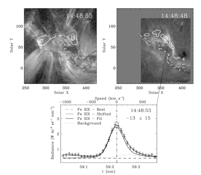
Figure 8: Gradual phase at a time when the CDS slit was crossing the western footpoint. The top left panel show a TRACE image in the 17.1 nm band while the H$\alpha$ image closest in time is shown on the top right panel. On the TRACE image isocontours of the Fe xix radiance at levels of (0.11, 0.22) W m^-2 sr^-1 are indicated by thick white solid lines. On the H$\alpha$ image, instead, the white thick contours refer to a RHESSI image obtained between 14:50 and 14:51 UTC in the 6 to 12 keV band. The contours are traced at levels of 40 % and 75 % of the maximum. The Fe xix line profile shown on the bottom panel is obtained by integrating over the areas within white solid thin lines in the H$\alpha$ image (area B). In this case the radiance of the rest component (dashed line) was set to zero. The dotted line indicate the background (lines plus constant background) defined from pre-flare spectra. The thick solid line indicate the fitted profile.

A coronal plasma heated above $10^{7}$ K in kernel B might explain the very different behaviour displayed by the two footpoints, both in radiance and velocity. In A, after the end of the impulsive phase, both coronal signatures undergo a rapid decay, while in B the radiance of Fe xix continues its increase up to 15:05 UTC, i.e., well into the gradual phase. The Fe xvi shows a similar trend, but with a more significant delay, reaching its maximum radiance in B almost one hour after the GOES peak. This seems consistent with the rapid cooling of “hot” plasma ($>10^{7}$ K), evaporated during the impulsive phase, to Fe xix temperatures, and successively, to values characteristic of Fe xvi emission.

In this same footpoint, downward directed motions are measured in both Fe xix and Fe xvi around the time of their peak emission, although the amplitudes are close to the error level (for Fe xix, (20 to 70 $\pm\leavevmode\nobreak\ 50$) km s^-1 for a double-component fitting and (6 $\pm$ 12) km s^-1 for a single-component fit; for Fe xvi, (20 $\pm\leavevmode\nobreak\ 12$) km s^-1). Downflows of $\approx(20\pm$ 9) km s^-1, are further observed in O v to outline the B footpoint around the time of maximum O v emission during the gradual phase ($\approx$15:42 UTC). No obvious downflows are instead measured in A during the gradual phase.

Finally, combining gradual phase RHESSI data with CDS measurements up to 14:50 UTC, we evaluate the contribution of the evaporated chromospheric plasma in filling the flare loops. Using the Fe xix data, we can estimate the total number of electrons transported with evaporation during the impulsive phase, assuming a symmetric evaporation on the two footpoints:

$$N_{up}=n_{\rm e}\leavevmode\nobreak\ 2\leavevmode\nobreak\ S_{cor}\leavevmode\nobreak\ f\leavevmode\nobreak\ v_{cor}\leavevmode\nobreak\ \Delta t,$$ (1)

where $n_{\rm e}$ is the electron density of the upflowing plasma, $f$ the coronal filling factor, $2\leavevmode\nobreak\ S_{cor}$ the area of the observed upflows (both footpoints), $v_{cor}$ the velocity, and $\Delta t$ the duration of the evaporation. The electron density and the upward velocity are the same as in § 4.2 (see also Eq. 5) and depend on whether we use one ($v_{cor}=-125$ km s^-1) or two ($v_{cor}=-240$ km s^-1) components to fit the Fe xix line profile at 14:42:03 UTC and upon the assumed iron abundance. We assume such densities and velocities as typical throughout the evaporation. $2\leavevmode\nobreak\ S_{cor}=2\times 1.2\times\leavevmode\nobreak\ 10^{18}$ cm² accounts for the fact that the plasma is flowing from both footpoints. Finally, $\Delta t=300$ s is taken equal to the duration of chromospheric downflows, for which we have a better temporal resolution.

With these values, for the two cases of single and double fitting and for both iron abundances of 7.5 and 8.1, we obtain the minimum and maximum estimate of $N_{up}=$ [3.8,10.]$\times 10^{37}\sqrt{f}$ electrons.

The above values can be compared with the total number of electrons in the entire loop system after the end of the evaporation phase. This can be written as:

$$N_{loop}=\sqrt{\frac{EM_{RHESSI}}{f\leavevmode\nobreak\ S_{cor}\leavevmode\nobreak\ L_{loop}}}f\leavevmode\nobreak\ S_{cor}\leavevmode\nobreak\ L_{loop},$$ (2)

where $EM_{RHESSI}=0.8\times 10^{48}$ cm^-3 is the emission measure obtained from the RHESSI spectrum at 15:13 UTC (only thermal component, see Fig. 9). From the TRACE images around 16:20 UTC a loop length $L_{loop}$ of $\approx 9.2\times 10^{9}$ cm can be derived, from which $N_{loop}=9.4\times 10^{37}\sqrt{f}$ electrons. Since both $N_{up}$ and $N_{loop}$ have the same dependence on $\sqrt{f}$, the evaporated material can account for 40 % up to 100 % of the material inside the loop system. This implies that the evaporated plasma largely contribute to the density of the post-flare loops.

Figure 9: RHESSI spectra in the 4 to 10 keV energy range at 14:50 UTC (left panel) and at 15:13 UTC (right panel). Notice the presence of a broadened emission feature at about 6.6 keV corresponding to a group of emission lines due to Fe xxiv – xxvi.

6 Cooling of post-flare loops

The whole evolution of the flare outlines the filling of magnetic loops by plasma evaporated from the chromosphere during the impulsive phase. Such loops become visible in all of our signatures during the extended gradual phase, with progressively cooler features appearing at later times (see Fig. 3). Fig. 10 reports the typical temperatures corresponding to our signatures, assumed as those corresponding to the maximum of the contribution function, vs. the peak time of the loop radiances. Moreover, the temperature of the thermal spectrum used to fit RHESSI data is also reported at the two times of acquisition.

We compare here the temporal evolution defined by the data with the results of the analytical formulae provided by Cargill et al. (1995) for the cooling time of a flare plasma. The first RHESSI spectrum at 14:50 UTC still shows a non-thermal component (see § 5), suggesting further energy input at the beginning of the gradual phase. Hence we begin the analysis of the cooling at 15:13 UTC, when RHESSI shows only a thermal component. The first data point corresponds to a $T\approx 8\times 10^{6}$ K, and an average electron density of $8.5\times 10^{9}$ cm^-3 (for $f=1$). We used the formulae provided for the static case since after 15:13 UTC no evaporative motions are visible anymore. The calculations were performed following two different approaches.

In the first case a constant density was assumed throughout the entire cooling period and the complete radiative loss function of Rosner et al. (1978) was used in the calculations. For this purpose Eqs. 7S and 8S of Cargill et al. (1995) have been generalised to any value of the exponent $\alpha$ of the power law. Using such equations, we computed the time until when conduction dominates over radiation. The temperature evolution of the cooling plasma was obtained through Eq. 3a of Cargill et al. (1995) before this time and Eq. 4 after, with the appropriate values for each piece of the radiative loss function of Rosner et al. (1978). The thin lines in Fig. 10 show the results of these calculations for three values of the filling factor $f$ (0.1, dot-dashed; 0.3, dashed; 0.5, dotted). The solid part of the curves indicates the times when conduction dominates, while the non-solid part indicates the time when the plasma cools radiatively.

In the second approach we assumed that the density is constant only during the conductive phase while $n\propto\sqrt{T}$ in the radiative phase (Serio et al., 1991). We also assumed the simplified radiative loss function $P_{rad}=1.7\times 10^{-19}n^{2}T^{-1/2}$ that fits, within a factor two, the CHIANTI radiative loss function for coronal abundances for $5\leavevmode\nobreak\ \leq\leavevmode\nobreak\ \log(T/{\rm K})\leavevmode\nobreak\ \leq\leavevmode\nobreak\ 7$. During the time dominated by conduction, the calculations are similar to the previous case. After this time, being $\alpha=-0.5$, we can use Eq. 6 of Cargill et al. (1995) to calculate the temperature evolution during the time when radiative cooling dominates. The results are represented by the thick curves in Fig. 10, for the same values of $f$. Again, the solid part represent the conductive cooling while the non-solid part is the radiative one.

Both approaches show that the observed curve can be explained by the cooling of the hot flare plasma injected into the loop system only if a volumetric filling factor of $\approx$ 0.2 to 0.5 is assumed, a value well in agreement with the estimated filling factors of cooling loops given by Aschwanden et al. (2003). We notice that the estimated cooling time in the temperature range $4\leavevmode\nobreak\ \leq\leavevmode\nobreak\ \log(T/{\rm K})\leavevmode\nobreak\ \leq\leavevmode\nobreak\ 5$ is much shorter than the observed one. This is expected because our initial assumptions are no longer valid in this range, in particular due to recombination of hydrogen.

7 Conclusions

We presented comprehensive observations of a small eruptive flare (GOES class C2.3) that developed on 2002 August 11 in NOAA region 10061. A wide array of instruments and diagnostics allowed us to follow the evolution of the flare from the chromosphere to the corona during both the impulsive phase and the long gradual phase. The eruption of a portion of a filament, located on the apparent magnetic inversion line, was signalled by an upward velocity of about $-30$ km s^-1 detected at 14:36:33 UTC by CDS in the O v line. A few minutes later the footpoints of a large loop system, subsequently visible also in the TRACE images, began to brighten in all signatures, reaching their maximum brightness around 14:42 UTC.

Figure 10: Cooling curve obtained from the time of maximum appearance of progressively colder features. RHESSI temperature at 14:50 UTC refers to the thermal component (see left panel of Fig. 9). Each set of curves (thin and thick) refer to three different values of the volumetric filling factor $f$ (0.1, dot-dashed; 0.3, dashed; 0.5, dotted). The solid part of the curves indicates the times when conduction dominates, while the non-solid part indicates the time when the plasma cools radiatively. The thick curves are obtained assuming constant density only during the conductive phase, while the thin curves are obtained assuming constant density through the entire cooling (see text).

During the impulsive phase of the flare, large coronal upflows of $-200$ km s^-1 or more are measured from the Doppler shift of the Fe xix line profiles on the ribbons at the footpoints of the flaring loop system. Interestingly, the two footpoints show quite a different behaviour. Footpoint A shows a fast (within our time resolution) rise of the radiances of all our signatures, followed by a slower decay of the Fe xvi and Fe xix emission. On this footpoint, during the impulsive phase, we can select a small area (3 CDS pixels) where a blue-shifted component clearly dominates the Fe xix profile. Upward motions of about $-70$ km s^-1 (likely underestimated) are also measured from the Fe xvi CDS data. These coronal upward motions occur in the location where downflows are observed in the O v and He i lines for at least 200 s but, unfortunately, no H$\alpha$ Dopplergrams are available for this footpoint.

On footpoint B instead, the radiances of Fe xix and Fe xvi lines increase very slowly and reach their maxima respectively 20 min and 60 min after the start of the flare. RHESSI data at 14:50 UTC show the emission in the 3 to 12 keV band to be mainly associated to this footpoint, with the spectrum indicating a temperature of the thermal component of 10.4 MK, i.e. larger than the Fe xix formation temperature (8 MK). This would explain the slow rise of Fe xix and Fe xvi radiances as due to progressive cooling of this “hot” plasma. During the impulsive phase, the blue-shifted and the stationary component of the Fe xix line profile on this area are of comparable strength, and no clear motion is measured from the Fe xvi line. The O v and He i lines show downward ($\approx 20$ km s^-1) motions outlining the flaring kernels. For this footpoint, within the FOV of the UBF imager, we observed simultaneous H$\alpha$ downflows that we estimated to be about ($7\pm 3$) km s^-1. To our knowledge, this is the first time that co-spatial, co-temporal, oppositely directed flows during the impulsive phase of a flare are measured in low chromosphere and corona, supporting the model of explosive chromospheric evaporation.

Such direct measurement gave us the possibility to compare the “instantaneous” momenta of the coronal and chromospheric moving plasma, whose equality is required in the hypothesis of explosive evaporation. We found that such momenta are equal within one order of magnitude. Previous works (Zarro et al., 1988; Canfield et al., 1990a) verified the equality of the momenta within the same limits using data without spatial resolution and integrating over the whole impulsive phase. Although we can utilise spatially resolved data, it remains very difficult to obtain more accurate estimates of the momentum balance, due to the inherent uncertainties in physical parameters such as coronal electron density and abundances, chromospheric hydrogen density and condensation height. To improve the knowledge of these parameters a larger number of spectral lines both in the EUV (including density diagnostics) and in visible/near-infrared (to build a semi-empirical model of the chromosphere) are necessary. However, this is likely to jeopardise the temporal and spatial resolution needed to study the impulsive phase of a flare. New space instruments with larger effective areas, such as the forthcoming EIS on Solar B, should improve the situation on the EUV side.

A further element in support of the chromospheric evaporation was given by RHESSI data acquired during the gradual phase, from which we obtained an estimate of the mass in the coronal loop system. Combining the velocity and radiance data from CDS, we could also estimate the mass evaporated during the impulsive phase of the flare, and found that it provided a large contribution to the density of the X-ray emitting coronal material.

Finally, during the extended gradual phase, the magnetic loops filled by evaporated plasma become visible in all of our spectral lines and band-passes, with progressively cooler features appearing at later times. The observed temporal evolution can be reproduced using the analytical formulae of Cargill et al. (1995). Initially the cooling is dominated by conduction, while radiative losses take over later on. A cooling time comparable to the observed one can be obtained only assuming a volumetric filling factor of $\approx$ 0.2 to 0.5. This in turn is consistent with the the presence of multiple thin loops heated successively, suggested by the observed dominant blue-shifted component in the Fe xix line profile only when we can use a small area to obtain reliable data.

To end this paper, we would like to make some remarks about the complexity of the TR behaviour. While our observations show downflows in the flaring kernels also from TR lines, in qualitative agreement with some hydrodynamical simulations of explosive evaporation (Fisher et al., 1985a, b), we note that recent hydrodynamic models of chromospheric evaporation (Allred et al., 2005) always predict upflows for the TR plasma. Several observations obtained with CDS during the impulsive phase of flares, with programs privilegeing either the spatial or the temporal resolution, offer a wide range of results. Upflows have been reported by Teriaca et al. (2003), using an observational sequence similar to the one presented in this paper, and Brosius (2003), that adopted a very high cadence program, but with a narrow field of view and limited spatial resolution. Upflow is also measured in our data during the impulsive phase, in the eastern footpoint nearby the area A but not appear to be obviously connected to the coronal upflows.. Downflows are instead reported by Brosius & Phillips (2004), using the same observing program as Brosius (2003), and Kamio et al. (2005) that analyse four flares in a larger FOV but with intermediate temporal resolution. Although at much lower spatial and temporal resolution, the same contradictory indications were obtained with SMM and OSO-8 instruments (see the discussion in Teriaca et al., 2003). It is likely that the behaviour of the TR is strongly related to the structure of the atmosphere depending upon the local magnetic topology. Space observations with substantially higher spatial resolution than now ($\leq 1^{\prime\prime}$) are most likely necessary to better understanding the dynamics of the TR and provide constraints to theoretical models. Further, we would like to point out that hydrodynamical simulations are generally computed for energetic flares (GOES class X-M) with a much harder spectrum for the impinging electrons ($\gamma$ from 4 to 6) than normally observed with RHESSI ($\gamma$ from 7 to 10) in small flares such as the one studied here.

Appendix A Momenta calculation. 

We give here a detailed description of equations and physical parameters used to calculate the downward and upward momenta $P_{down}$ and $P_{up}$.

The mass density can be written as $\rho=\mu m_{\rm p}\leavevmode\nobreak\ n_{T}$, where $\mu$ is the mean particle weight, $m_{\rm p}=1.67\times 10^{-24}$ g is the proton mass, and $n_{T}$ the total particle number density. For a fully-ionised plasma of hydrogen with 10 % helium, $\mu=0.61$ and $n_{T}=1.91\leavevmode\nobreak\ n_{\rm e}$, while for a neutral gas, $\mu=1.27$ and $n_{T}=1.1\leavevmode\nobreak\ n_{\rm H}$, where $n_{\rm H}$ is the hydrogen number density. Downflow momentum in the chromosphere (neutral gas) can then be written as:

$$P_{down}=1.27\leavevmode\nobreak\ m_{\rm p}\leavevmode\nobreak\ 1.1\leavevmode\nobreak\ n_{ch}\leavevmode\nobreak\ S_{ch}\leavevmode\nobreak\ v_{ch}\leavevmode\nobreak\ \Delta h\leavevmode\nobreak\ f_{ch},$$ (3)

where $n_{ch}$ is the pre-flare chromospheric hydrogen density, assumed to be (2.2 to 4.0)$\times 10^{13}$ cm^-3 from model VAL F (Vernazza et al., 1981). The area $S_{ch}$ with detectable chromospheric downflows is $2.5\times 10^{17}$ cm². Within this area, the average downflow velocity, $v_{ch}$, is about ($7\pm 3$) km s^-1. $\Delta h$ represents the thickness of the chromospheric condensation. We assume that $\Delta\leavevmode\nobreak\ h$ between a lower limit of $\approx 100$ km, given by dynamic simulations (Abbett & Hawley, 1999) and an upper limit of 200 km, obtained in semi-empirical models of a small flare that includes the velocity fields (Falchi & Mauas, 2002). Finally, $f_{ch}$ is the chromospheric filling factor. Since the spatial scale of the H$\alpha$ images is $0.5\arcsec$ per pixel, smaller than the size of the velocity patches in the chromosphere ($2\arcsec$ to $3\arcsec$), we assume $f_{ch}=1$. With these values, we obtain $5.1\times\leavevmode\nobreak\ 10^{19}$ g cm s${}^{-1}\leavevmode\nobreak\ \leq\leavevmode\nobreak\ P_{down}\leavevmode\nobreak\ \leq\leavevmode\nobreak\ 4.6\times\leavevmode\nobreak\ 10^{20}$ g cm s^-1. The lower and upper limits refer to the minimum and maximum values for the hydrogen density ($n_{ch}$), $v_{ch}$, and $\Delta\leavevmode\nobreak\ h$.

At coronal level, the momentum of the upflowing plasma is given by:

$$P_{up}=0.61\leavevmode\nobreak\ m_{p}\leavevmode\nobreak\ 1.91\leavevmode\nobreak\ n_{\rm e}\leavevmode\nobreak\ S_{cor}\leavevmode\nobreak\ L\leavevmode\nobreak\ f\leavevmode\nobreak\ v_{cor},$$ (4)

with $n_{\rm e}$ given by

$$n_{\rm e}=\sqrt{\frac{EM}{f\leavevmode\nobreak\ S_{cor}\leavevmode\nobreak\ L}}.$$ (5)

In the above equations $S_{cor}$ is the area of the region from where blue-shifted profiles arise, $L$ the thickness of the emitting region, $f$ the coronal filling factor, $v_{cor}$ the plasma speed at coronal level, and $EM$ the emission measure computed from the observed radiance using the CHIANTI database (Dere et al., 1997; Landi et al., 1999) with ionisation equilibrium calculations from Mazzotta et al. (1998).

The radiance of the Fe xix 59.2 nm line is proportional to ${n_{\rm e}}^{2}$ for $8\leavevmode\nobreak\ \leq\leavevmode\nobreak\ \log\leavevmode\nobreak\ n_{\rm e}/{\rm cm^{-3}}\leavevmode\nobreak\ \leq\leavevmode\nobreak\ 12$ and it is, hence, suitable for emission measure calculation. The iron abundance $A_{[\rm Fe]}$ is 8.1 in the corona (Feldman et al., 1992). However, because the plasma is ablated from the chromosphere, the photospheric abundance of 7.6 (Grevesse & Sauval, 1998) may also apply. Thus, we will assume an abundance varying between 7.5 and 8.1.

Coronal upflows are measured in eleven effective CDS pixels, so $S_{cor}=1.2\times\leavevmode\nobreak\ 10^{18}$ cm². $L$ is taken to vary between 1.1$\times 10^{9}$ cm ($=\sqrt{S_{cor}}$) and 2$\times 10^{9}$ cm (obtained estimating the geometrical depth of the flaring loop along the line of sight, assuming the loop is perpendicular to the solar surface). The electron density, $n_{\rm e}$, of the evaporating plasma (from the emission measure) and the coronal velocity, $v_{cor}$, depend on whether the Fe xix spectra are fitted with one or two components. The computed values of $n_{\rm e}$ are between $3\times 10^{9}$ and $8\times 10^{9}$ cm^-3 for $f$=1. Finally, we note that in the extreme case of magnetic flux tubes not expanding with height, the ratio $S_{ch}/S_{cor}$ yields a lower limit of $f=0.2$, so we assume $0.2\leavevmode\nobreak\ \leq\leavevmode\nobreak\ f\leavevmode\nobreak\ \leq\leavevmode\nobreak\ 1$.

For both values of $f$, $P_{up}$ is calculated with the values of $EM$ and $v_{cor}$ obtained in both cases of single and double component fitting and for both estimates of $L$ and $A_{[\rm Fe]}$. The maximum and minimum of the sixteen obtained values are taken to give $5.9\times\leavevmode\nobreak\ 10^{19}$ g cm s${}^{-1}\leavevmode\nobreak\ \leq\leavevmode\nobreak\ P_{up}\leavevmode\nobreak\ \leq\leavevmode\nobreak\ 4.9\times\leavevmode\nobreak\ 10^{20}$ g cm s^-1.

References

- Abbett & Hawley (1999) Abbett, W. P. & Hawley, S. L. 1999, ApJ, 521, 906
- Allred et al. (2005) Allred, J.C., Hawley, S. L., Abbett, W. P., & Carlsson, M. 2005, ApJ, 630, 573
- Antonucci et al. (1982) Antonucci, E., Gabriel, A. H., Acton, L. W., Leibacher, J. W., Culhane, J. L., Rapley, C. G., Doyle, J. G., Machado, M. E., & Orwig, L. E. 1982, Sol. Phys., 78, 107
- Aschwanden et al. (2003) Aschwanden, M.J., Schrijver, C.J., Winebarger, A.R., & Warren, H.P. 2003, ApJL, 588, L49
- Bentley et al. (1994) Bentley, R. D., Doschek, G. A., Simnett, G. M., Rilee, M. L., Mariska, J. T., Culhane, J. L., Kosugi, T., & Watanabe, T. 1994, ApJ, 421, L55
- Brosius (2003) Brosius, J. W. 2003, ApJ, 586, 1417
- Brosius & Phillips (2004) Brosius, J. W., & Phillips, K. J. H. 2004, ApJ, 613, 580
- Canfield et al. (1990a) Canfield, R. C., Metcalf, T. R., Zarro, D. M., & Lemen, J. R. 1990a, ApJ, 348, 333
- Canfield et al. (1990b) Canfield, R. C., Penn, M. J., Wulser, J. P., & Kiplinger, A. L. 1990b, ApJ, 363, 318
- Cargill et al. (1995) Cargill, P. J., Mariska, J. T., & Antiochos, S. K. 1995, ApJ, 439, 1034
- Culhane et al. (1991) Culhane, J. L., et al. 1991, Sol. Phys., 136, 89
- Czaykowska et al. (1999) Czaykowska, A., De Pontieu, B., Alexander, D., & Rank, G. 1999, ApJ, 521, L75
- Del Zanna & Mason (2005) Del Zanna, G., Mason, H. E. 2005, A&A, 433, 731
- Del Zanna et al. (2002) Del Zanna, G., Gibson, S. E., Mason, H. E., Pike, C. D., & Mandrini, C. H. 2002, Adv. Space Res., 30, 551
- Dere et al. (1997) Dere, K. P., Landi, E., Mason, H. E., Monsignori Fossi, B. C., & Young, P. R. 1997, A&AS, 125, 149
- Doschek et al. (1980) Doschek, G. A., Feldman, U., Kreplin, R. W. & Cohen, L. 1980, ApJ, 239, 725
- Emslie et al. (1992) Emslie, A. G., Li, P., & Mariska J. T. 1992, ApJ 399, 714
- Falchi et al. (1992) Falchi, A., Falciani, R., & Smaldone, L.A. 1992, A&A, 256, 255
- Falchi et al. (1997) Falchi, A., Qiu, J., & Cauzzi, G. 1997, A&A, 328, 371
- Falchi & Mauas (2002) Falchi, A., & Mauas, P. J. D 2002, A&A, 387, 678
- Feldman et al. (1992) Feldman, U., Mandelbaum, P., Seely, J. L., Doschek, G. A., & Gursky H., 1992, ApJS, 81, 387
- Fisher et al. (1985a) Fisher, G., Canfield, R., & McClymont, A. 1985a, ApJ, 289, 414
- Fisher et al. (1985b) Fisher, G., Canfield, R., & McClymont, A. 1985b, ApJ, 289, 434
- Forbes & Acton (1996) Forbes, T., & Acton, L. W. 1996, ApJ, 459, 330
- Forbes (2003) Forbes, T. 2003, Adv. Space Res., 32, 1043
- Gan et al. (1991) Gan, W., Zhang, H., & Fang, C. 1991, A&A, 241, 618
- Gan et al. (1995) Gan, W. Q., Cheng, C.C, & Fang, C. 1995, ApJ 452, 445
- Gan & Watanabe (1997) Gan, W. Q., & Watanabe, T. 1997, Sol. Phys., 174, 403
- Grevesse & Sauval (1998) Grevesse, N., & Sauval, A.J. 1998, Spa. Sci. Rev., 85, 161
- Handy et al. (1999) Handy, B., Acton, L., Kankelborg, C., Wolfson, C., Akin, D., Bruner, M., Caravalho, R., Catura, R., Chevalier, R., Duncan, D., & coauthors, . 1999, Sol. Phys., 187, 229
- Hannah et al. (2004) Hannah, I. G., Christe, S., Krucker, S., Hudson, H. S., Fletcher, L., & Hendry, M. A. 2004, in Soho 15, Coronal heating, ed. D. Danesy, ESA-SP (Noordwijk, The Netherlands: ESA-SP), 575, 259
- Harrison et al. (1995) Harrison, R., Sawyer, E., Carter, M., Cruise, A., Cutler, R., Fludra, A., Hayes, R., Kent, B., Lang, J., Parker, D., & coauthors, . 1995, Sol. Phys., 162, 233
- Hori et al. (1998) Hori, K., Yokoyama, T., Kosugi, T., & Shibata, K. 1998, ApJ, 500, 492
- Kamio et al. (2005) Kamio, S., Kurokawa, H., Brooks, D. H., Kitai, R., & Ueno, S. 2005, ApJ 625, 1027
- Klimchuk et al. (1988) Klimchuk, J., Sturrock, P., & Yang, W.-H. 1988, ApJ, 335, 456
- Kopp & Pneuman (1976) Kopp, R. A. & Pneuman, G. W. 1976, Sol. Phys., 50, 85
- Krucker et al. (2002) Krucker, S., Christe, S., Lin, R., Hurford, G., & Schwartz, R. 2002, Sol. Phys., 210, 445
- Landi et al. (1999) Landi, E., Landini, M., Dere, K. P., Young, P. R., & Mason, H. E., 1999, A&AS, 135, 339
- Lin et al. (2002) Lin, R., Dennis, B., Hurford, G., Smith, D., Zehnder, A., Harvey, P., Curtis, D., Pankow, D., Turin, P., Bester, M., & coauthors, . 2002, Sol. Phys., 210, 3
- Maltagliati et al. (2006) Maltagliati, L., Falchi, A., & Teriaca, L. 2006, Sol. Phys., 235, 125
- Mariska et al. (1989) Mariska, J., Emslie, A., & Li, P. 1989, ApJ, 341, 1067
- Mazzotta et al. (1998) Mazzotta, P., Mazzitelli, G., Colafrancesco, S., & Vittorio, N. 1998, A&AS, 133, 403
- Moore et al. (1980) Moore, R., McKenzie, D. L., Svestka, Z., Widing, K. G., Dere, K. P., Antiochos, S. K., Dodson-Prince, H. W., Hiei, E., Krall, K. R., & Krieger, A. S. 1980, in Solar Flares: A Monograph from Skylab Solar Workshop II, ed.P. Sturrock, 341
- Neupert (1968) Neupert, W. 1968, ApJ, 153, L59
- Petschek (1964) Petschek, H. 1964, in NASA-SP, Vol. 50, The Physics of Solar Flares [, Proceedings of the AAS-NASA Symposium held 28-30 October, 1963 at the Goddard Space Flight Center, Greenbelt, MD, ed. W. Hess (Washington: NASA), 425
- Phillips (2004) Phillips, K. J. H., 2004, ApJ, 605, 921
- Rosner et al. (1978) Rosner, R., Tucker, W. H., & Vaiana, G. S. 1978, ApJ, 220, 643
- Scherrer et al. (1995) Scherrer, P., Bogart, R., Bush, R., Hoeksema, J., Kosovichev, A., Schou, J., Rosenberg, W., Springer, L., Tarbell, T., Title, A., & coauthors 1995, Sol. Phys., 162, 129
- Schmieder et al. (1998) Schmieder, B., Fang, C., & Harra-Murnion, L.K. 1998, Sol. Phys., 182, 447
- Serio et al. (1991) Serio, S., Reale, F., Jakimiec, J., Sylwester, B., & Sylwester, J. 1991, A&A, 241, 197
- Shibata (1996) Shibata, K. 1996, Adv. Spa. Res., 17, 9
- Teriaca et al. (2003) Teriaca, L., Falchi, A., Cauzzi, G., Falciani, R., Smaldone, L. A., & Andretta, V. 2003, ApJ, 588, 596
- Vernazza et al. (1981) Vernazza, J. E., Avrett, E. H., & Loeser, R. 1981, ApJS, 45, 635
- Warren & Doschek (2005) Warren, H. P., & Doschek, G. A. 2005, ApJ, 618, L157
- Wülser et al. (1994) Wülser, J. P., et al. 1994, ApJ, 424, 459
- Zarro et al. (1988) Zarro D. M., Canfield R. C., Strong K. T., & Metcalf T. R. 1988, ApJ, 324, 582