Technical Naturalness on a Codimension-2 Brane

Abstract:

We compute how threshold effects obtained by integrating out a heavy particle localized on a codimension-2 brane influence the properties of the brane and the bulk fields it sources in $D=d+2$ dimensions. We do so using a recently developed formalism for matching the characteristics of higher codimension branes to the properties of the bulk fields they source. We show that although the dominant heavy-mass dependence induced in the low-energy codimension-2 tension has the generic size expected, $T_{2}\propto M^{d}$, the very-low-energy effective potential governing the on-brane curvature once bulk KK modes are integrated out can be additionally suppressed, by factors of order $\kappa^{2}M^{d}$, where $\kappa$ is the bulk gravitational coupling. In the special case of a codimension-2 brane in a 6D supersymmetric bulk we also estimate the size of the contributions of short-wavelength bulk loops near the brane, and find these can be similarly suppressed.

1 Introduction

Much of modern thinking in particle physics about what should be expected to replace the Standard Model at LHC energies is driven by the idea that the Standard Model is an effective description of some unknown, more fundamental, theory describing physics at shorter distance scales, $\lambda=1/M$, than we can presently measure. This picture captures much of what makes the Standard Model most attractive: it consists of the most general set of interactions that are possible among the observed particles (plus the Higgs boson) that involve only couplings having (engineering) dimension (mass)^d for $d\geq 0$ [1]. This is just what one would expect to describe any physics in the more fundamental theory that is unsuppressed by powers of $1/M$.

What does not fit easily into this picture, however, are the only two interactions allowed by the model that have dimensionful couplings:

$$\mathcal{L}_{\rm rel}=-\sqrt{-g}\,\left[m^{4}-\mu^{2}H^{\dagger}H\right]\,,$$ (1)

where $H$ is the Higgs doublet. The problem with these is that agreement with observations requires the scales $m$ and $\mu$ to be much smaller than $M$, unlike what usually happens in low-energy effective theories. Since such suppression of so-called relevant operators is unusual, this difficulty is made into a virtue by using it as a clue to guide our search for whatever the new physics is that ultimately replaces the Standard Model. Since both of the terms in eq. (1) arise in the scalar potential, one is led by these kinds of considerations to regard systems that can handle and suppress contributions to scalar potentials as particularly interesting candidates for the Standard Model’s short-distance (UV) completion. All of the most promising theories proposed so far — supersymmetric theories, models without scalar fields and extra-dimensional scenarios — are of this type.

It is the purpose of this paper to try to understand in more detail one of the remarkable ways extra-dimensional models can suppress ultra-violet contributions to scalar potentials. As as been noticed by many authors — first within the context of cosmic string back-reaction [2] in four dimensions, and then again for brane-world models in codimensions one [3] and two [4, 5] — extra-dimensional field equations allow codimension two branes in extra dimensions to have precisely flat induced geometries. This, despite having significant nonzero homogeneous energy densities (or tensions), and being coupled to higher dimensional gravity. By contrast, if there were no extra dimensions, a nonzero space-filling constant energy density would inevitably curve the geometry of spacetime when coupled to gravity. This observation that the induced brane geometry can be decoupled from its on-brane energy density provides one of the very few potential ways forward for understanding how it is that the observed acceleration of the universe points to an energy density, $m^{4}$, with $m$ so much smaller than almost all of the other scales found in the Standard Model [6].

Although the existence of higher dimensional solutions whose 4D curvature is decoupled from the brane tension is suggestive, what has been missing to date is a quantitative study of precisely how (or if) the scalar potential in the low-energy effective theory manages to remain insensitive to the integrating out of high-energy scales. In particular if a higher dimensional scalar field couples to the brane in addition to gravity, it is important to understand under what circumstances the low energy action describing the system has interesting special properties, similar to the ones previously mentioned in the case of pure gravity. In this paper we provide part of this missing analysis, by explicitly integrating out (at one loop) a very massive brane field on a codimension-2 brane, to see how this affects the low-energy effective theory. We use for these purposes a scalar tensor theory in a $D=d+2$-dimensional bulk coupled in a fairly generic way to a $d$-dimensional codimension-2 brane, for which the matching rules between brane properties and near-brane bulk asymptotics have recently been worked out, following an effective approach, in [7].

We find the following results

• Integrating out a brane field of mass $M$ generically contributes an amount $M^{d}$ to the tension, $T_{2}$, of a space-filling codimension-2 brane in $d+2$ dimensions, and so is not suppressed relative to naive expectations.

• This tension does not necessarily imply a similarly large contribution to the effective potential, $U_{2}$, in the $d$-dimensional effective theory that governs the spacetime curvatures at energies well below the Kaluza-Klein scale. When the bulk is integrated out at the classical level, these results are consistent with the existence, in extra-dimensional theories, of flat solutions with nonzero tensions.

• By examining theories with scalar fields in the bulk we are able to see that the situations where the low-energy curvatures can be small are also those for which the codimension-2 brane has little or no coupling to the bulk scalar, in agreement with the known situations where large tensions coexist with flat on-brane geometries.

• In order to contrast the behaviour of codimension-2 sources with those of the better-studied codimension-1 branes, we use a representation of the codimension-2 brane in terms of a small regularizing codimension-1 brane that encircles the position of the codimension-2 object at a small radius $\rho_{b}$ [16, 7]. From the point of view of the low-energy effective theory, on scales much larger than $\rho_{b}$, the main difference between such a regularizing brane and a macroscopic codimension-1 brane is that the radius $\rho_{b}$ is not a macroscopically observable variable, and it will therefore be integrated out. As we will explain, at the classical level this amounts to self-consistently determine $\rho_{b}$ in terms of the various fields in the low-energy theory by solving the brane junction conditions, including those of gravity.

• It is this relaxation of $\rho_{b}$ that, in certain circumstances, is ultimately responsible for the suppression of the contribution of the codimension-2 tension to the low-energy on-brane curvature. In general, $\rho_{b}$ adjusts itself to ensure that the effective potential, $U_{2}$, defined below the Kaluza scale is completely determined by the brane tension, $T_{2}(\phi)$, regarded as a function of the bulk scalar evaluated at the brane position (given explicitly by eq. (18), of later sections). In particular, as we will explain, the solution for $U_{2}$ strictly vanishes when $T_{2}^{\prime}={\hbox{d}}T_{2}/{\hbox{d}}\phi=0$, as required by what is known about the back-reaction of codimension-2 pure tension branes. More generally, if $T_{2}^{\prime}$ is nonzero but small, then $U_{2}$ is suppressed by factors of order $\kappa^{2}T_{2}^{\prime}$, where $\kappa$ is the higher-dimensional Planck scale in the bulk.

The above results arise in a calculation which evaluates loop effects due to integrating out brane fields at the quantum level, but only integrates out bulk fields (and in particular $\rho_{b}$) within the bulk classical approximation. A crucial question therefore asks how bulk loops might change the above picture. We close the paper by taking a step in this direction by estimating the contributions of the most dangerous (short-wavelength) bulk loops within the more specific context where the bulk is six-dimensional and supersymmetric. This extends earlier calculations of the ultraviolet sensitivity of bulk loops far from the brane, to include the effects of loops that are close to the branes. We find that, for the contributions examined, supersymmetry can suppress bulk loops to be of order the Kaluza-Klein scale, again representing a significant suppression to the low-energy potential $U_{2}$.

We organize our presentation as follows. §2 starts by reviewing the brane-bulk matching conditions for codimension-2 branes, as recently derived in ref. [7]. This section in particular describes how the codimension-2 brane can be regularized in terms of a small codimension-1 brane, and relates the properties of each to the other. §3 then adds a massive field to the brane and integrates it out at one loop, keeping track of how this loop changes its interactions with the bulk fields. §4 finally combines the results of the earlier sections, by specializing them to the simple case where the brane-bulk couplings are exponentials in the bulk scalar. The size of both the codimension-2 brane tension, $T_{2}$, and the low-energy effective scalar potential, $U_{2}$, are computed, both before and after integrating out the massive brane field. We conclude in §5.

2 The Framework

We work for illustrative purposes within a higher-dimensional scalar-tensor theory that provides the simplest context for displaying our calculations. Since our interest is in integrating out heavy matter on codimension-2 branes, we focus primarily on the situations of space-filling $d$-dimensional branes sitting within a $D=(d+2)$-dimensional bulk spacetime. The particular case of $d=4$ and $D=6$ is of particular interest, as the simplest ‘realistic’ case within which the impact of higher-dimensional ideas on technical naturalness might be relevant in practice.

2.1 Bulk field equations

Consider the following bulk action, governing the interactions between the $D=(d+2)$-dimensional metric, $g_{{\scriptscriptstyle M}{\scriptscriptstyle N}}$ and a real scalar field, $\phi$:

$$S_{\scriptscriptstyle B}=-\frac{1}{2\kappa^{2}}\int\mathrm{d}^{D}x\sqrt{-g}\;\left[\,g^{{\scriptscriptstyle M}{\scriptscriptstyle N}}\Bigl{(}{\cal R}_{{\scriptscriptstyle M}{\scriptscriptstyle N}}+\partial_{\scriptscriptstyle M}\phi\,\partial_{\scriptscriptstyle N}\phi\Bigr{)}\right]+S_{{\scriptscriptstyle GH}}\,,$$ (2)

where ${\cal R}_{{\scriptscriptstyle M}{\scriptscriptstyle N}}$ denotes the Ricci tensor built from $g_{{\scriptscriptstyle M}{\scriptscriptstyle N}}$ and $S_{{\scriptscriptstyle GH}}=\kappa^{-2}\int_{\partial M}{\hbox{d}}^{D-1}x\sqrt{-\gamma}\;K$, denotes the Gibbons-Hawking action [9], which is required when using the Einstein field equations in the presence of boundaries (as we do below). Here $\gamma_{mn}$ denotes the induced metric on the boundary, and $K=\gamma^{mn}K_{mn}$ is the trace of the boundary’s extrinsic curvature. (Since we are also interested in the case of higher-dimensional supergravity, which also involve Maxwell and Kalb-Ramond fields, and nontrivial scalar potentials, $V=V_{0}\,e^{\phi}$ [10], in section §4 we discuss the extent to which these features change our results.)

The corresponding field equations are

$$\Box\phi=0\quad\hbox{and}\quad{\cal R}_{{\scriptscriptstyle M}{\scriptscriptstyle N}}+\partial_{\scriptscriptstyle M}\phi\,\partial_{\scriptscriptstyle N}\phi=0\,.$$ (3)

In the immediate vicinity of a codimension-2 brane we imagine the bulk fields to take an axially (transverse) and maximally (on-brane) symmetric form

$$\mathrm{d}s^{2} = \mathrm{d}\rho^{2}+\hat{g}_{mn}\,\mathrm{d}x^{m}\mathrm{d}x^{n}$$ (4)

$$= \mathrm{d}\rho^{2}+e^{2B}\,\mathrm{d}\theta^{2}+e^{2W}g_{\mu\nu}\,\mathrm{d}x^{\mu}\,\mathrm{d}x^{\nu}\,,$$

where $\rho$ denotes proper distance transverse to the brane, $\theta\simeq\theta+2\pi$ is the angular coordinate encircling the brane, and the functions $B$, $W$ and $\phi$ are functions of $\rho$ only. The on-brane metric, $g_{\mu\nu}$, is a $d$-dimensional maximally symmetric Minkowski-signature metric depending only on $x^{\mu}$.

Accidental bulk symmetries

The field equations, eqs. (3), enjoy two accidental symmetries, whose interplay with brane interactions will be explored in the following:

• Axion symmetry: The axion symmetry is defined by

  $$\phi\to\phi+\zeta\,,$$ (5)

  for constant $\zeta$, with $g_{{\scriptscriptstyle M}{\scriptscriptstyle N}}$ held fixed.

• Scaling symmetry: A scaling symmetry of the field equations is

  $$g_{{\scriptscriptstyle M}{\scriptscriptstyle N}}\to\lambda^{2}g_{{\scriptscriptstyle M}{\scriptscriptstyle N}}\,,$$ (6)

  with constant $\lambda$, and $\phi$ held fixed.

Both of these symmetries take solutions of the classical field equations into distinct new solutions of the same equations, but need not be respected by the couplings of the bulk fields to any space-filling source branes, whose properties we next describe.

2.2 Brane properties

We imagine the bulk to be sprinkled with a number of space-filling codimension-2 source branes, whose back-reaction dominates the asymptotic near-brane behaviour of the bulk fields. In a derivative expansion, their low-energy brane-bulk interactions are governed by the action

$$S_{b}=-\int\mathrm{d}^{d}x\,\sqrt{-\gamma}\;\Bigl{[}T_{2}(\phi)+X_{2}(\phi)\,\partial^{\mu}\phi\,\partial_{\mu}\phi+Y_{2}(\phi)\,R+\cdots\Bigr{]}\,,$$ (7)

where $\gamma_{\mu\nu}$ denotes the induced metric on the brane and the subscript ‘2’ emphasizes that the brane has codimension 2 (by contrast with a codimension-1 branes to be considered shortly). The ellipses represent further terms that arise at low energies in a derivative expansion.

This brane action breaks the axion symmetry, eq. (5), if any of the coefficients, $T_{2}$, $X_{2}$ or $Y_{2}$, depend on $\phi$. The tension term, $T_{2}$, also breaks the scaling symmetry, eq. (6), unless $T_{2}$ is constant. The higher-derivative terms always break the scaling symmetry, but can preserve a diagonal combination of eqs. (5) and (6) corresponding to $\lambda^{2}=e^{a\zeta}$ provided $X_{2},Y_{2}\propto e^{a\phi}$.

At still lower energies the dynamics of the bulk-brane system is normally dominated by very light modes, that are massless within the purely classical approximation. These include the low-energy $d$-dimensional metric, $g_{\mu\nu}$, possibly together with a variety of moduli, $\varphi$, coming from $\phi$ or the metric components. The dynamics of these modes below the Kaluza-Klein (KK) scale is governed by a different effective $d$-dimensional theory,

$$S_{\rm eff}=-\int\mathrm{d}^{d}x\,\sqrt{-g}\;\left[U_{\rm eff}(\varphi)+\frac{1}{2\kappa_{4}^{2}}\,R+\cdots\right]\,,$$ (8)

obtained by integrating out all bulk KK modes as well as any heavy brane states. At the purely classical level this action is obtained by eliminating these states as functions of the light fields using their classical equations of motion, and so depend on the details of the classical bulk action.

In the classical approximation the contribution of the branes to $S_{\rm eff}$ takes a simple form. The accidental symmetries guarantee the existence (classically) of a massless scalar mode corresponding to shifts of $\phi$, so $\phi(\rho)=\varphi+\delta\phi(\rho)$. The low-energy potential, $U_{\rm eff}$, turns out to arise as a sum over local terms, each evaluated at the position of a brane [7]:

$$U_{\rm eff}(\varphi)=\frac{1}{d}\sum_{b}U_{2}[\phi(\rho_{b};\varphi)]\,.$$ (9)

The fact that $U_{2}$ (defined more explicitly below) can vanish even when $T_{2}\neq 0$ is what allows codimension-2 branes having nonzero tension to have flat on-brane geometries [4, 5].

2.3 Brane-bulk matching

It is the quantities $T_{2}(\phi)$ and $U_{2}(\phi)$ that dictate the near-brane behaviour of bulk fields, through the matching conditions. For our purposes, assuming the brane of interest to be situated at $\rho=0$, these become (see [12, 7] for a complete discussion):

$$\lim_{\rho\to 0}\left(e^{B+dW}\partial_{\rho}\phi\right) = \frac{\kappa^{2}T_{2}^{\prime}}{2\pi}$$

$$\lim_{\rho\to 0}\left(e^{B+dW}\partial_{\rho}W\right) = \frac{\kappa^{2}U_{2}}{2\pi d}$$ (10)

$$\lim_{\rho\to 0}\left(e^{B+dW}\partial_{\rho}B\right) = 1-\frac{\kappa^{2}}{2\pi}\left[T_{2}+\left(\frac{d-1}{d}\right)U_{2}\right]\,.$$

Codimension-1 regularization

A drawback of eqs. (2.3) is the dependence of the right-hand-side on quantities like $\phi(\rho=0)$, that need not be well-defined if $\phi$ diverges as one approaches the brane positions. This can be dealt with by defining an alternative, renormalized, codimension-2 brane action, as discussed in [7, 13, 14] by elaborating on the work [15]. On the other hand, for the aim of the present work, it is convenient to simply regularize this divergence through the artifice of replacing the codimension-2 brane with a very small cylindrical codimension-1 brane, situated at $\rho=\rho_{b}$ [12, 7, 16], with the interior geometry ($\rho<\rho_{b}$) capped off with a smooth solution to the bulk field equations (see fig. 1). We use capital latin indices, $x^{\scriptscriptstyle M}$, to describe all $D=d+2$ coordinates at once, reserving lower-case indices, $x^{m}$, for coordinates on the $(d+1)$-dimensional codimension-1 brane, and greek indices, $x^{\mu}$, for the $d$ codimension-2 brane directions.

The action on this codimension-1 brane is chosen to be

$$S_{\rm reg}=-\int\mathrm{d}^{d+1}x\,\sqrt{-\gamma}\;\Bigl{[}T_{1}(\phi)+Z_{1}(\phi)\,\partial^{m}\sigma\,\partial_{m}\sigma+\cdots\Bigr{]}\,,$$ (11)

where $\sigma$ is a massless, on-brane mode, whose presence is included in order to dynamically support the brane radius at nonzero $\rho$ against its propensity to collapse gravitationally. This is done by choosing for its classical solution a configuration that winds around the brane, $\sigma=n\theta$, for $n$ a nonzero integer.

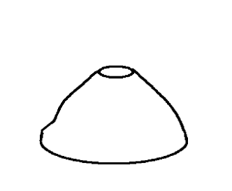
Figure 1: The regularized near-brane cap geometry.

In terms of this action the codimension-2 tension is obtained directly by dimensional reduction in the $\theta$ direction. Using $e^{B(\rho_{b})}=\rho_{b}$, this leads to

$$T_{2}(\phi,\rho_{b})=2\pi\rho_{b}\left[T_{1}(\phi)+\frac{n^{2}}{2\rho_{b}^{2}}\,Z_{1}(\phi)\right]\,.$$ (12)

As for the codimension-2 action, this preserves the axionic symmetry, eq. (5), if $T_{1}$ and $Z_{1}$ are $\phi$ independent. However, because $\rho_{b}\to\lambda\rho_{b}$ there is no choice for $T_{1}$ which preserves the scaling symmetry, eq. (6). The diagonal combination with $\lambda=e^{-a\zeta}$ survives if $T_{1}\propto e^{a\phi}$ and $Z_{1}\propto e^{-a\phi}$.

The brane contribution, $U_{2}$, to the low-energy potential can also be computed in terms of $T_{1}$ and $Z_{1}$ by classically integrating out the bulk KK modes explicitly. This integration involves evaluating the classical action at the classical solution, with the result regarded as a function of the low-energy zero modes, $g_{\mu\nu}$ and $\varphi$. Keeping in mind that the only nonzero part of the action, eq. (2), is in this case the Gibbons-Hawking term, $S_{\scriptscriptstyle GH}$, and that this receives opposite-sign contributions from outside and inside the codimension-1 brane, one obtains a result that depends only on the jump conditions [17] evaluated at the brane position

$$S_{\rm eff}(\varphi)=\left(S_{{\scriptscriptstyle B}}+\sum_{b}S_{\rm reg}\right)_{\phi^{\rm cl}(\varphi),g^{\rm cl}_{{\scriptscriptstyle M}{\scriptscriptstyle N}}(\varphi)} = \sum_{b}\left\{S_{\rm reg}-\frac{1}{\kappa^{2}}\int\mathrm{d}^{d+1}x\,\sqrt{-\hat{g}}\;\Bigl{[}K\Bigr{]}_{b}\right\}$$ (13)

$$= \sum_{b}\left\{S_{\rm reg}-\frac{1}{d}\int\mathrm{d}^{d+1}x\,\sqrt{-\hat{g}}\;\hat{g}_{mn}T^{mn}\right\}\,,$$

where $\Bigl{[}X\Bigr{]}_{b}=\lim_{\epsilon\to 0}\Bigl{[}X(\rho_{b}+\epsilon)-X(\rho_{b}-\epsilon)\Bigr{]}$. $\sqrt{-\hat{g}}\;T^{mn}=2\,\delta S_{\rm reg}/\delta\hat{g}_{mn}$ is the stress tensor of the codimension-1 brane, whose independent components are

$$T_{\mu\nu}=-\left(T_{1}+\frac{n^{2}}{2\rho_{b}^{2}}\,Z_{1}\right)\hat{g}_{\mu\nu}\quad\hbox{and}\quad T_{\theta\theta}=-\left(T_{1}-\frac{n^{2}}{2\rho_{b}^{2}}\,Z_{1}\right)\hat{g}_{\theta\theta}\,.$$ (14)

Eq. (13) implies each brane contributes to the very-low-energy theory as if its codimension-1 Lagrangian density were

$$\hat{\cal L}_{\rm reg}={\cal L}_{\rm reg}-\frac{2}{d}\,\hat{g}_{mn}\,\frac{\delta S_{\rm reg}}{\delta\hat{g}_{mn}}\,.$$ (15)

Once compactified in the $\theta$ direction, this gives the following brane contribution to $U_{2}$ [7]:

$$U_{2}(\phi,\rho_{b})=-2\pi\rho_{b}\left[T_{1}(\phi)-\frac{n^{2}}{2\rho_{b}^{2}}\,Z_{1}(\phi)\right]=2\pi\rho_{b}\,g^{\theta\theta}T_{\theta\theta}\,.$$ (16)

Finally, the expression for $\rho_{b}(\phi)$ is obtained by integrating the ($\rho\rho$) Einstein equation, which expresses the ‘Hamiltonian’ constraint for integrating the bulk field equations in the $\rho$ directions [18, 12]:

$$U_{2}\left[\frac{4\pi}{\kappa^{2}}-2T_{2}-\left(\frac{d-1}{d}\right)U_{2}\right]-\left(T_{2}^{\prime}\right)^{2}\simeq 0\,,$$ (17)

and the approximate equality involves dropping terms that are of order $\rho_{b}^{2}R$ relative to those displayed. Such curvature terms are always negligible in the limit where the brane size, $\rho_{b}$, is much smaller than the bulk radius of curvature to which it gives rise.

Eq. (17) states that the solution $\rho_{b}(\phi)$ adjusts itself to ensure that $U_{2}(\phi)=U_{2}(\phi,\rho_{b}(\phi))$ is not independent of $T_{2}(\phi)=T_{2}(\phi,\rho_{b}(\phi))$. Expanding in powers of $\kappa^{2}$, we find

$$\frac{\kappa^{2}U_{2}}{2\pi} = \left(\frac{d}{d-1}\right)\left\{\left(1-\frac{\kappa^{2}T_{2}}{2\pi}\right)-\left[\left(1-\frac{\kappa^{2}T_{2}}{2\pi}\right)^{2}-\left(\frac{d-1}{d}\right)\left(\frac{\kappa^{2}T_{2}^{\prime}}{2\pi}\right)^{2}\right]^{1/2}\right\}$$ (18)

$$\simeq \frac{1}{2}\left(1-\frac{\kappa^{2}T_{2}}{2\pi}\right)^{-1}\left(\frac{\kappa^{2}T_{2}^{\prime}}{2\pi}\right)^{2}+\cdots\,.$$

The second line here emphasizes that the root is chosen to ensure that $U_{2}$ vanishes in the limit when $T_{2}^{\prime}\to 0$, since this limit corresponds to rugby-ball type geometries [4, 5] having flat on-brane spacetimes ($U_{2}=0$) with nonzero but $\phi$-independent tensions ($T_{2}^{\prime}=0$). It is simple to see that all the corrections in higher powers of $\kappa^{2}$, contained in the dots, are proportional to $T_{2}^{\prime}$.

Solving eq. (17) to lowest order in $\kappa^{2}$ leads to the condition $U_{2}\simeq 0$, and so

$$\rho_{b}^{2}(\phi)\simeq\frac{n^{2}Z_{1}(\phi)}{2T_{1}(\phi)}\,,$$ (19)

showing that, in the limit in which gravity is weak, $\rho_{b}$ adjusts itself to try to set $U_{2}$ to zero. Using this solution, we can integrate out the quantity $\rho_{b}$, and the codimension-2 brane tension becomes

$$T_{2}(\phi)=T_{2}(\phi,\rho_{b}(\phi))\simeq 2\pi|n|\sqrt{2\,T_{1}(\phi)Z_{1}(\phi)}\,.$$ (20)

This expression then allows $U_{2}$ to be computed from eq. (17) or (18) to next-to-leading order in $\kappa^{2}$, giving [7]

$$U_{2}(\phi)=U_{2}(\phi,\rho_{b}(\phi))\simeq\frac{\kappa^{2}}{4\pi}\,\left(T_{2}^{\prime}\right)^{2}=\left(\frac{\pi n^{2}\kappa^{2}}{2}\right)\frac{\left[\left(T_{1}Z_{1}\right)^{\prime}\right]^{2}}{T_{1}Z_{1}}\,.$$ (21)

As mentioned earlier, the function $U_{2}(\phi)$ vanishes when the brane tension $T_{2}$ does not depend on the field $\phi$. Looking at the first of equations (2.3), we see that having $T_{2}$ be $\phi$-independent also requires the dilaton derivative to vanish as one approaches the brane. Since such derivatives naturally vanish when the brane is located in a region where $\phi$ has a constant, or approximately constant, profile in the bulk, it is natural to find that branes with $\phi$-independent tensions are commonly the sources for geometries having such regions. This observation will turn out to be useful in the following.

2.4 An Example

For later purposes we pause here to record the above steps for an interestingly broad example. We choose for this purpose the case where $T_{1}$ and $Z_{1}$ are exponentials:

$$T_{1}(\phi)=A_{\scriptscriptstyle T}e^{-a_{t}\phi}\qquad\hbox{and}\qquad Z_{1}(\phi)=A_{\scriptscriptstyle Z}e^{-a_{z}\phi}\,,$$ (22)

and so

$$T_{2}(\phi,\rho_{b})\simeq 2\pi\left[\rho_{b}A_{\scriptscriptstyle T}e^{-a_{t}\phi}+\left(\frac{n^{2}A_{\scriptscriptstyle Z}}{2\rho_{b}}\right)e^{-a_{z}\phi}\right]\,,$$ (23)

and

$$U_{2}(\phi,\rho_{b})\simeq-2\pi\left[\rho_{b}A_{\scriptscriptstyle T}e^{-a_{t}\phi}-\left(\frac{n^{2}A_{\scriptscriptstyle Z}}{2\rho_{b}}\right)e^{-a_{z}\phi}\right]\,.$$ (24)

In this case the zeroth-order brane size is

$$\rho_{b0}=|n|\sqrt{\frac{A_{\scriptscriptstyle Z}}{2A_{\scriptscriptstyle T}}}\,e^{-(a_{z}-a_{t})\phi/2}\,.$$ (25)

Using these, the leading contribution to the codimension-2 brane tension and on-brane potential then become

$$T_{2}(\phi)\simeq{T_{2}}_{0}(\phi)=2\pi|n|\sqrt{2A_{\scriptscriptstyle T}A_{\scriptscriptstyle Z}}\,e^{-(a_{t}+a_{z})\phi/2}\,,$$ (26)

and

$$U_{2}(\phi)\simeq\frac{\kappa^{2}}{4\pi}\left({{T_{2}}_{0}}^{\prime}\right)^{2}=\frac{\pi}{2}\,n^{2}(a_{t}+a_{z})^{2}\kappa^{2}A_{\scriptscriptstyle T}A_{\scriptscriptstyle Z}e^{-(a_{t}+a_{z})\phi}\,.$$ (27)

Recall that these choices always break the scaling symmetry, eq. (6), provided at least one of $A_{\scriptscriptstyle T}$ or $A_{\scriptscriptstyle Z}$ is nonzero. They respect the axionic symmetry, eq. (5), if and only if $a_{t}=a_{z}=0$. Finally, they preserve a diagonal combination of these two symmetries if $a_{t}+a_{z}=0$. Notice that in this last case $T_{2}$ is $\phi$-independent, and so eq. (18) shows $U_{2}=0$ solves the constraint (17) to all orders in $\kappa^{2}$.

3 Integrating out a Massive Brane Field

We next investigate the stability of the above considerations to ultraviolet effects on the brane. The simplest way to do so is to explicitly integrate out a heavy brane-localized field, and see how the brane-bulk connection changes as a result.

3.1 The brane field

To this end, consider supplementing the brane action with new term describing a massive real scalar field, $\psi$. Since our goal is to see how this changes the bulk-brane interaction, we regard $\psi$ as being localized on the codimension-1 regularized brane, and so take $S_{\rm reg}\to S_{\rm reg}+S(\psi)$ with

$$S(\psi)=-\frac{1}{2}\int\mathrm{d}^{(d+1)}x\;\sqrt{-\hat{g}}\Bigl{[}P(\phi)(\partial\psi)^{2}+m_{\star}^{2}Q(\phi)\,\psi^{2}\Bigr{]}\,.$$ (28)

Here $m_{\star}$ is a constant having dimensions of mass, and if we adopt $z=\rho_{b}\theta$ as coordinate in the periodic direction, then all fields satisfy the boundary condition $\psi(z)=\psi(z+L)$, with $L=2\pi\rho_{b}$.

For the purposes of computing quantum corrections, we imagine starting with a classical solution whose induced metric on the codimension-2 brane is flat, making the metric on the codimension-1 regularizing brane

$${\hbox{d}}s^{2}=e^{2W_{b}}\eta_{\mu\nu}\,{\hbox{d}}x^{\mu}{\hbox{d}}x^{\nu}+\rho_{b}^{2}{\hbox{d}}\theta^{2}\,.$$ (29)

It is convenient at this point to re-scale $e^{W_{b}}$ into $x^{\mu}$, so that ${\hbox{d}}s^{2}=\eta_{mn}\,{\hbox{d}}x^{m}{\hbox{d}}x^{n}$ where we take the coordinate in the angular direction to be $x^{d}=z$. As discussed above, such a flat classical background would arise, for instance, if $T_{1}=A_{\scriptscriptstyle T}e^{-a_{t}\phi}$ and $Z_{1}=A_{\scriptscriptstyle Z}e^{-a_{z}\phi}$ with $a_{z}=-a_{t}$.

Provided $P\neq 0$ the $\psi$-particle action always breaks the scaling symmetry, eq. (6), but preserves the axionic symmetry if and only if $P$ and $Q$ are $\phi$-independent. A diagonal subgroup of these two symmetries can be preserved when $P$, $Q$, $T_{1}$ and $Z_{1}$ are all exponentials,

$$P(\phi)=A_{\scriptscriptstyle P}\,e^{-a_{p}\,\phi}\quad\hbox{and}\quad Q(\phi)=A_{\scriptscriptstyle Q}\,e^{-a_{q}\phi}\,,$$ (30)

provided $a_{p}=a_{z}=-a_{q}=-a_{t}$. The effective mass of $\psi$ for observers on the brane is $\phi$-dependent, given explicitly by

$$m^{2}(\phi)=\frac{m_{\star}^{2}\,Q(\phi)}{P(\phi)}\,,$$ (31)

and so $m^{2}=m_{\star}^{2}(A_{\scriptscriptstyle Q}/A_{\scriptscriptstyle P})e^{-(a_{q}-a_{p})\phi}$ when $P$ and $Q$ are exponentials, à la eqs. (30).

The stress energy for this heavy scalar is given by

$$T_{mn}(\psi)=P(\phi)\partial_{m}\psi\partial_{n}\psi-\frac{1}{2}\,g_{mn}\,\Bigl{[}P(\phi)(\partial\psi)^{2}+m_{\star}^{2}Q(\phi)\,\psi^{2}\Bigr{]}\,,$$ (32)

which satisfies

$${T^{m}}_{m}(\psi)=-\left(\frac{d-1}{2}\right)P(\phi)(\partial\psi)^{2}-\left(\frac{d+1}{2}\right)\,m_{\star}^{2}Q(\phi)\,\psi^{2}$$ (33)

in $d$ spacetime dimensions on the codimension-2 brane (with $d=4$ being the case of most direct interest).

3.2 Quantum Contributions

To assess the contribution of quantum effects on the brane, we integrate out $\psi$ by computing the Gaussian functional integral

$$\exp\Bigl{[}i\Gamma(\phi,g)\Bigr{]}=\int{\cal D}\psi\;\exp\Bigl{[}iS(\psi,\phi,g)\Bigr{]}\,,$$ (34)

so that $\int{\cal D}\psi\;e^{i[S_{\rm reg}+S(\psi)]}=e^{i[S_{\rm reg}+\Gamma]}$. Eq. (34) may be evaluated by differentiating with respect to $\phi$, giving

$$\frac{\delta\Gamma}{\delta\phi}=-\frac{1}{2}\sqrt{-\hat{g}}\left[\frac{P^{\prime}}{P}\,\langle P\,(\partial\psi)^{2}\rangle+\frac{Q^{\prime}}{Q}\,\langle m_{\star}^{2}Q\,\psi^{2}\rangle\right]\,,$$ (35)

where $\langle X(\psi)\rangle=e^{-i\Gamma}\int{\cal D}\psi\,X(\psi)\,e^{iS}$.

As described in Appendix A, the relevant expectation values can be expressed as

$$\langle P(\phi)\partial_{\mu}\psi\partial_{\nu}\psi\rangle=\frac{\eta_{\mu\nu}}{2L^{d+1}}\int_{0}^{\infty}\frac{\mathrm{d}t}{t^{(d+2)/2}}\;e^{-\lambda t}\vartheta_{3}(it)=\eta_{\mu\nu}\,\frac{I_{1+d/2}(\lambda)}{2L^{d+1}}\,,$$ (36)

and

$$\langle P(\phi)(\partial_{z}\psi)^{2}\rangle=-\frac{i}{L^{d+1}}\int_{0}^{\infty}\frac{\mathrm{d}t}{t^{d/2}}\;e^{-\lambda t}\vartheta_{3}^{\prime}(it)=-\frac{J_{d/2}(\lambda)}{L^{d+1}}\,,$$ (37)

and

$$\langle m_{\star}^{2}Q(\phi)\,\psi^{2}\rangle=\frac{\lambda}{L^{d+1}}\int_{0}^{\infty}\frac{\mathrm{d}t}{t^{d/2}}\;e^{-\lambda t}\vartheta_{3}(it)=\frac{\lambda I_{d/2}(\lambda)}{L^{d+1}}\,,$$ (38)

where

$$\lambda(\phi)=\frac{m^{2}(\phi)L^{2}}{4\pi}=\frac{m_{\star}^{2}L^{2}\,Q(\phi)}{4\pi P(\phi)}=\pi\rho_{b}^{2}m^{2}(\phi)\,.$$ (39)

The properties of the functions $I_{\alpha}(\lambda)$ and $J_{\alpha}(\lambda)$ are spelt out in detail in Appendix B. They satisfy a very useful identity,

$$\Bigl{\langle}P(\phi)\,\partial_{m}\psi\,\partial^{m}\psi+m_{\star}^{2}Q(\phi)\,\psi^{2}\Bigr{\rangle}=\frac{1}{L^{d+1}}\left[\frac{d}{2}\,I_{1+d/2}(\lambda)-J_{d/2}(\lambda)+\lambda I_{d/2}(\lambda)\right]=0\,,$$ (40)

which (as is proven in Appendix A) is a consequence of our use of dimensional regularization.

Quantum fluctuations in $\psi$ contribute to the brane stress-energy tensor, $T_{mn}\to T_{mn}+\Bigl{\langle}T_{mn}(\psi)\Bigr{\rangle}$, where

$$\Bigl{\langle}T_{mn}(\psi)\Bigr{\rangle} = \frac{2}{\sqrt{-\hat{g}}}\,\frac{\delta\Gamma}{\delta\hat{g}^{mn}}=\Bigl{\langle}P(\phi)\,\partial_{m}\psi\,\partial_{n}\psi\Bigr{\rangle}-\frac{1}{2}\,\hat{g}_{mn}\,\Bigl{\langle}P(\phi)\,(\partial\psi)^{2}+m_{\star}^{2}Q(\phi)\,\psi^{2}\Bigr{\rangle}$$ (41)

$$= \Bigl{\langle}P(\phi)\,\partial_{m}\psi\,\partial_{n}\psi\Bigr{\rangle}\,,$$

which uses the identity, eq. (40). Its components evaluate to

$$\Bigl{\langle}T_{\mu\nu}(\psi)\Bigr{\rangle} = \eta_{\mu\nu}\;\frac{I_{1+d/2}(\lambda)}{2L^{d+1}}$$

$$\hbox{and}\quad\Bigl{\langle}T_{zz}(\psi)\Bigr{\rangle} = -\frac{J_{d/2}(\lambda)}{L^{d+1}}=-\frac{[\lambda I_{d/2}(\lambda)+\frac{d}{2}I_{1+d/2}(\lambda)]}{L^{d+1}}\,,$$ (42)

and, again using eq. (40), its trace is

$$\Bigl{\langle}{T^{m}}_{m}(\psi)\Bigr{\rangle} = -\left(\frac{d-1}{2}\right)\Bigl{\langle}P(\phi)\,(\partial\psi)^{2}\Bigr{\rangle}-\left(\frac{d+1}{2}\right)\,\Bigl{\langle}m_{\star}^{2}Q(\phi)\,\psi^{2}\Bigr{\rangle}$$ (43)

$$= \Bigl{\langle}P(\phi)\,(\partial\psi)^{2}\Bigr{\rangle}=-\Bigl{\langle}m_{\star}^{2}Q(\phi)\,\psi^{2}\Bigr{\rangle}=-\frac{\lambda I_{d/2}(\lambda)}{L^{d+1}}\,,$$

which (naively) vanishes when $m_{\star}=0$, and so is completely given by any trace anomaly when this is nonzero. In particular, notice that $m_{\star}=0$ implies $\langle{T^{m}}_{m}\rangle=0$ when $d=2k$ is a positive even integer, since in this case the codimension-1 brane has odd dimension and so the divergent parts of the above expressions vanish in dimensional regularization (see Appendix A for details).

3.3 Codimension-2 quantities

For the present purposes, of most interest is the contribution of $\psi$ loops to low energy quantities, so we next seek the loop contribution to the codimension-2 quantities $T_{2}$ and $U_{2}$. This involves repeating their earlier derivation with the replacements $S_{\rm reg}\to S_{\rm reg}+\Gamma$ and $T_{mn}\to T_{mn}+\langle T_{mn}(\psi)\rangle$.

The most direct means for computing both $T_{2}$ and $U_{2}$ then uses their representation as compactifications of components of the stress tensor — $T_{2}=-L\,g^{tt}T_{tt}$ and $U_{2}=L\,g^{\theta\theta}T_{\theta\theta}$ — which summarize eqs. (12), (14) and (16). These remain true provided $T_{mn}\to T_{mn}+\langle T_{mn}(\psi)\rangle$, suggesting that the change generated by $\psi$ loops is

$$\Delta T_{2}(\phi,L)=L\langle T_{tt}\rangle=-\frac{I_{1+d/2}(\lambda)}{2L^{d}}\,,$$ (44)

and

$$\Delta U_{2}(\phi,L)=L\langle T_{zz}\rangle=-\frac{J_{d/2}(\lambda)}{L^{d}}=-\frac{[\lambda I_{d/2}(\lambda)+\frac{d}{2}I_{1+d/2}(\lambda)]}{L^{d}}\,.$$ (45)

Notice in particular that the $\phi$-dependence of these quantities (at fixed $L$) only enters through the combination $m^{2}(\phi)\propto Q/P$.

A check on these expressions comes if we instead work directly with the loop contributions to the regularized brane action, $S_{\rm reg}=\int\mathrm{d}^{d+1}x\,\sqrt{-\hat{g}}\;{\cal L}_{\rm reg}$. Writing $S_{\rm reg}+\Gamma=\int\mathrm{d}^{d+1}x\,\sqrt{-\hat{g}}\;({\cal L}_{\rm reg}+\Delta{\cal L}_{\rm reg})$, eq. (35) implies

$$\frac{\partial\Delta{\cal L}_{\rm reg}}{\partial\phi}=\frac{1}{2}\left[\frac{P^{\prime}}{P}-\frac{Q^{\prime}}{Q}\right]\langle m_{\star}^{2}Q\,\psi^{2}\rangle=-\frac{1}{2m^{2}}\left(\frac{\partial m^{2}}{\partial\phi}\right)\frac{\lambda I_{d/2}(\lambda)}{L^{d+1}}\,,$$ (46)

which uses $(P^{\prime}/P)-(Q^{\prime}/Q)=[\ln(P/Q)]^{\prime}=-(1/m^{2})(\partial m^{2}/\partial\phi)$, eq. (38) and eq. (40). Finally, provided $\partial m^{2}/\partial\phi\neq 0$ this integrates to

$$\Delta{\cal L}_{\rm reg}=-\frac{1}{2L^{d+1}}\int^{\lambda}\mathrm{d}\hat{\lambda}\,I_{d/2}(\hat{\lambda})=\frac{I_{1+d/2}(\lambda)}{2L^{d+1}}\,,$$ (47)

where the integral is performed using $\int^{\lambda}\mathrm{d}\hat{\lambda}\,I_{\alpha}(\hat{\lambda})=-I_{1+\alpha}(\lambda)$. Finally, dimensional reduction gives $\Delta T_{2}=-L\,\Delta{\cal L}_{\rm reg}$, in agreement with eq. (44).

Figure 2: The function $U_{2}(\lambda)+\Delta U_{2}(\lambda)$ vs $\lambda$.

Similarly, integrating out the bulk KK modes at the classical level using $S_{\rm reg}+\Gamma$ as the regularized brane action, leads to loop corrections to the effective action for energies well below the transverse KK scale, as seen by observers residing on the brane. The change to these due to the $\psi$ loops is

$$\Delta S_{\rm eff}=\Gamma-\frac{1}{d}\int\mathrm{d}^{d+1}x\,\sqrt{-\hat{g}}\;\langle{T^{m}}_{m}\rangle\,,$$ (48)

showing that $\psi$ loops enter into this action both by directly changing the brane action, and by changing the junction conditions relevant to integrating out the bulk fields. Writing $\Delta S_{\rm eff}=\int{\hbox{d}}^{d}x\sqrt{-g}\;\Delta{\cal L}_{\rm eff}$ gives $\Delta{\cal L}_{\rm eff}=\int{\hbox{d}}z\left[\Delta{\cal L}_{\rm reg}-\frac{1}{d}\,\sqrt{-\hat{g}}\;\langle{T^{m}}_{m}\rangle\right]$, and so

$$\Delta{\cal L}_{\rm eff}=\frac{1}{L^{d}}\left[\frac{1}{2}\,I_{1+d/2}(\lambda)+\frac{\lambda}{d}\,I_{d/2}(\lambda)\right]=\frac{J_{d/2}(\lambda)}{dL^{d}}\,,$$ (49)

so using $\Delta U_{2}=-d\,\Delta{\cal L}_{\rm eff}$ agrees with eq. (45).

Finally, notice that the derivation of the curvature constraint, eq. (17), relating $U_{2}$ to $T_{2}$, goes through as before, but with $T_{mn}$ replaced everywhere by $T_{mn}+\langle T_{mn}(\psi)\rangle$. This guarantees that $U_{2}+\Delta U_{2}$ can be obtained from $T_{2}+\Delta T_{2}$ by using eq. (21), precisely as $U_{2}$ can from $T_{2}$.

The limit $mL\gg 1$

Before going further it is instructive to evaluate these for the asymptotic case where $mL\gg 1$, since this is particularly easy to interpret. Appendix B shows that when $\lambda\gg 1$ we have $I_{\alpha}(\lambda)\simeq\lambda^{\alpha-1/2}\Gamma\left(\frac{1}{2}-\alpha\right)$, and so

$$\Delta T_{2}\simeq-\frac{m^{d+1}L}{2(4\pi)^{(d+1)/2}}\;\Gamma\left(-\frac{1}{2}-\frac{d}{2}\right)\,,$$ (50)

and

$$\Delta U_{2}\simeq\frac{m^{d+1}L}{2(4\pi)^{(d+1)/2}}\;\Gamma\left(-\frac{1}{2}-\frac{d}{2}\right)\,.$$ (51)

Notice these satisfy $\Delta U_{2}=-\Delta T_{2}$, just as would be expected if both arose from a contribution to the codimension-1 brane tension,

$$\Delta T_{1}(\phi) \simeq -\frac{m^{d+1}}{2(4\pi)^{(d+1)/2}}\;\Gamma\left(-\frac{1}{2}-\frac{d}{2}\right)$$ (52)

$$\to \frac{m^{5}}{120\pi^{2}}\quad\hbox{as}\quad d\to 4\,,$$

where the limit $d\to 4$ uses $\Gamma\left(-\frac{5}{2}\right)=-\frac{8}{15}\,\sqrt{\pi}$. Indeed, when $\psi$ is very massive compared with the codimension-1 KK scale, $2\pi/L=1/\rho_{b}$, we expect its quantum effects are well captured by local contributions to the brane action, starting with $\Delta{\cal L}_{\rm reg}\simeq-\Delta T_{1}+$ (higher derivative terms). Furthermore, eq. (52) agrees with the large-$m$ limit of eq. (47).

In the general case eqs. (44) and (45) predict $\Delta T_{2}\neq-\Delta U_{2}$, implying they do not have an interpretation as simple as a contribution to $T_{1}$. This is because when $mL\mathrel{\raise 1.29167pt\hbox{$<$\kern-8.50006pt\lower 4.30554pt\hbox{$\sim$}}}1$ the wavelengths integrated out are similar to the size of the entire circular direction on the codimension-1 brane, and so need not depend only on local geometrical quantities. Their contributions must be local in the transverse dimensions, however, provided that their wavelength is much smaller than the typical scales set by the transverse geometry.

The limit $mL\to 0$

A second instructive limit corresponds to taking $mL\to 0$, for which Appendix B shows $I_{\alpha}(0)=2\pi^{\frac{1}{2}-\alpha}\,\Gamma\left(\alpha-\frac{1}{2}\right)\,\zeta\left(2\alpha-1\right)$. In this case eqs. (44), (45) and (47) become

$$\Delta T_{2}(\phi,L)\simeq\frac{\Delta U_{2}(\phi,L)}{d}\simeq-L\,\Delta{\cal L}_{\rm reg} \simeq -\frac{1}{\pi^{(d+1)/2}L^{d}}\,\Gamma\left(\frac{1}{2}+\frac{d}{2}\right)\,\zeta\left(d+1\right)$$ (53)

$$\to -\frac{3\,\zeta\left(5\right)}{4\pi^{2}L^{4}}\quad\hbox{as}\quad d\to 4\,.$$

Notice $d\Delta T_{2}\to\Delta U_{2}$ when $mL\to 0$, consistent with the result $\langle{T^{m}}_{m}\rangle\to 0$.

Eliminating $\rho_{b}$

After determining the expressions for $\Delta T_{2}(\phi,L)$ and $\Delta U_{2}(\phi,L)$, the final step amount to eliminate $L$ — or equivalently $\rho_{b}$ — in terms of $\phi$ by using eq. (17). To leading order in $\kappa^{2}$ this involves solving the condition $U_{2}(\phi,L)\simeq 0$, leading to eq. (19), $\rho^{2}_{b0}\simeq n^{2}Z_{1}/(2\,T_{1})$ in the absence of the quantum $\psi$ contributions.

For the purposes of computing the quantum correction $\delta\rho_{b}^{2}$, suppose $T_{1}\simeq M^{d+1}$ and $Z_{1}\simeq M^{d-1}$ are characterized by a common regularization mass scale $M$, and so eq. (19) implies $L_{0}=2\pi\rho_{b0}\simeq 2\pi n/M$. Since for us $\rho_{b}$ plays the role of an ultraviolet regulator, our interest in what follows is in the limit $mL_{0}=2\pi\rho_{b0}m\simeq 2\pi nm/M\ll 1$ and $m/M\ll 1$, in which case $d\,\Delta T_{2}(\phi,\rho_{b})\simeq\Delta U_{2}(\phi,\rho_{b})\simeq-c\,d/(2\pi\rho_{b})^{d}$ with $c=\Gamma\left(\frac{1}{2}+\frac{d}{2}\right)\zeta(d+1)\,\pi^{-(d+1)/2}$. Since in this limit we have

$$L_{0}T_{1}\sim L_{0}\left(\frac{n^{2}Z_{1}}{\rho_{b0}^{2}}\right)\sim 2\pi nM^{d}\quad\hbox{and}\quad\Delta U_{2}\sim\frac{d}{(2\pi L_{0}^{2})^{d/2}}\sim\frac{dM^{d}}{(2\pi)^{3d/2}n^{d}}\,,$$ (54)

it follows that $\left|\delta\rho_{b}^{2}\right|\ll\rho_{b0}^{2}$, provided that the inequality $(2\pi)^{1+3d/2}n^{d+1}\gg d$ is satisfied. Using this observation, we solve $U_{2}(\phi,\rho_{b})\simeq 0$ perturbatively in $\delta\rho_{b}^{2}$, to give

$$\frac{\delta\rho_{b}^{2}}{\rho_{b0}^{2}}\simeq-\frac{c\,d}{2\pi^{2}n^{2}Z_{1}(\phi)(2\pi\rho_{b0})^{d-1}}=-\frac{c\,d}{T_{1}}\left(\frac{T_{1}}{2\pi^{2}Z_{1}}\right)^{(d+1)/2}\,.$$ (55)

With this choice, the leading corrections to $T_{2}(\phi)$ become

$$T_{2}(\phi) = {T_{2}}_{0}[\phi,\rho_{b0}(\phi)]+\frac{\partial{T_{2}}_{0}}{\partial\rho_{b}}[\phi,\rho_{b0}(\phi)]\,\delta\rho_{b}+\Delta T_{2}[\phi,\rho_{b0}(\phi)]+\cdots$$ (56)

$$= 2\pi|n|\sqrt{2\,T_{1}(\phi)Z_{1}(\phi)}-\frac{c}{(2\pi|n|)^{d}}\left[\frac{2\,T_{1}(\phi)}{Z_{1}(\phi)}\right]^{d/2}+\cdots\,,$$

which uses ${T_{2}}_{0}(\phi,\rho_{b})=2\pi\rho_{b}T_{1}+\pi n^{2}Z_{1}/\rho_{b}$ and so $\partial{T_{2}}_{0}/\partial\rho_{b}\propto{U_{2}}_{0}(\phi,\rho_{b})$ vanishes when evaluated at $\rho_{b}=\rho_{b0}(\phi)$. In the previous expression, the dots contain corrections proportional to positive powers of $\kappa^{2}$.

Finally, the constraint, eq. (17), automatically ensures $U_{2}(\phi)$ satisfies eq. (18), and so

$$U_{2}(\phi)\simeq\frac{1}{2}\left(1-\frac{\kappa^{2}T_{2}}{2\pi}\right)^{-1}\left(\frac{\kappa^{2}T_{2}^{\prime}}{2\pi}\right)^{2}+\cdots\,,$$ (57)

up to higher powers of $(\kappa^{2}T_{2}^{\prime})^{2}$, with $T_{2}(\phi)$ given by eq. (56).

4 Technical Naturalness

We may now use the above tools to quantify how integrating heavy brane physics modifies properties of the low-energy world. We ask in particular how symmetry-breaking effects on the brane modify at low energies the symmetries of the bulk action. We use for this purpose both the scaling and axionic shift symmetries, eqs. (5) and (6), of the simplified bulk theory used for illustrative purposes here, but we have in mind applications to other symmetries like supersymmetry as well.

4.1 Brane Loops

With this in mind we work within the particularly interesting framework of exponential brane couplings to $\phi$, as described by eqs. (22) and (30) above: $T_{1}=A_{\scriptscriptstyle T}e^{-a_{t}\phi}$, $Z_{1}=A_{\scriptscriptstyle Z}e^{-a_{z}\phi}$, $P=A_{\scriptscriptstyle P}e^{-a_{p}\phi}$ and $Q=A_{\scriptscriptstyle Q}e^{-a_{q}\phi}$. In this case the leading contributions to $T_{2}(\phi)$ and $\rho_{b}(\phi)$ become

$${T_{2}}_{0}(\phi) = 2\pi|n|\sqrt{2A_{\scriptscriptstyle T}A_{\scriptscriptstyle Z}}\,e^{-(a_{t}+a_{z})\phi/2}$$

$$\hbox{and}\quad\rho_{b0}(\phi) = |n|\sqrt{\frac{A_{\scriptscriptstyle Z}}{2A_{\scriptscriptstyle T}}}\,e^{-(a_{z}-a_{t})\phi/2}\,,$$ (58)

and so ${U_{2}}_{0}\simeq\kappa^{2}(T_{2}^{\prime})^{2}/4\pi$ becomes

$${U_{2}}_{0}(\phi)\simeq\frac{\pi n^{2}}{2}\,\kappa^{2}(a_{t}+a_{z})^{2}A_{\scriptscriptstyle T}A_{\scriptscriptstyle Z}\;e^{-(a_{t}+a_{z})\phi}\,.$$ (59)

The $\psi$ mass, $m(\phi)$, is

$$m(\phi)=m_{\star}\sqrt{\frac{A_{\scriptscriptstyle Q}}{A_{\scriptscriptstyle P}}}\,e^{-(a_{q}-a_{p})\phi/2}\,,$$ (60)

and so

$$\lambda_{0}=\pi\rho_{b0}^{2}m^{2}\simeq\frac{\pi n^{2}m_{\star}^{2}}{2}\left(\frac{A_{\scriptscriptstyle Z}A_{\scriptscriptstyle Q}}{A_{\scriptscriptstyle T}A_{\scriptscriptstyle P}}\right)\,e^{-(a_{z}+a_{q}-a_{t}-a_{p})\phi}\,.$$ (61)

Provided $\lambda_{0}\ll 1$ the leading correction to the codimension-2 tension due to $\psi$ loops, eq. (56), becomes

$$\Delta T_{2}(\phi)\simeq-\frac{c}{(2\pi|n|)^{d}}\left[\frac{2A_{\scriptscriptstyle T}}{A_{\scriptscriptstyle Z}}\right]^{d/2}e^{-d(a_{t}-a_{z})\phi/2}$$ (62)

and so

$$\Delta U_{2}(\phi)\simeq\frac{\kappa^{2}}{4\pi}\,\left[\Delta T_{2}^{\prime}(\phi)\right]^{2}\simeq\frac{\kappa^{2}c^{2}d^{2}(a_{t}-a_{z})^{2}}{16\pi(2\pi|n|)^{2d}}\left[\frac{2A_{\scriptscriptstyle T}}{A_{\scriptscriptstyle Z}}\right]^{d}e^{-d(a_{t}-a_{z})\phi}$$ (63)

We consider now several important special cases.

The case $a_{t}=a_{q}:=a$ and $a_{z}=a_{p}:=a+2\,b$

This choice is motivated by a situation of practical interest where there exists a frame for which $\phi$ appears undifferentiated only as an overall power of $e^{\phi}$ pre-multiplying the entire brane action. That is, ${\cal L}_{\rm reg}(\phi,\partial_{m}\phi,g_{mn})=e^{-\alpha\phi}f(\partial_{m}\phi,\check{g}_{mn})$ for some metric $\check{g}_{mn}=e^{-2\beta\phi}g_{mn}$, implying $a_{t}=a_{q}=\alpha+d\,\beta$ and $a_{z}=a_{p}=\alpha+(d-2)\beta$, so $a=\alpha+d\,\beta$ and $b=-\beta$.

In this case we have $\rho_{b0}\propto e^{-b\phi}$ and $m\propto e^{b\phi}$ so $\lambda_{0}\propto m^{2}\rho_{b0}^{2}$ is $\phi$-independent. Then ${T_{2}}_{0}\propto e^{-(a+b)\phi}$, and the leading quantum correction $\Delta T_{2}\propto e^{db\phi}$ (regardless of whether $\lambda_{0}$ is large or small). There are then two special situations of particular interest:

1. The case $b=0$: This situation corresponds to it being the bulk Einstein frame for which the brane action has the form ${\cal L}_{\rm reg}(\phi,\partial_{m}\phi,g_{mn})=e^{-\alpha\phi}f(\partial_{m}\phi,g_{mn})$. In this case, if $A_{\scriptscriptstyle T}\sim M^{d+1}$ and $A_{\scriptscriptstyle Z}\sim M^{d-1}$ then we have ${T_{2}}_{0}\propto M^{d}e^{-a\phi}$ while $\Delta T_{2}\propto M^{d}/(2\pi n)^{2d}$ is precisely $\phi$-independent. Consequently in this case we have ${U_{2}}_{0}\sim\kappa^{2}M^{2d}a^{2}e^{-2a\phi}$, while $\Delta U_{2}$ precisely vanishes to leading order in $\kappa^{2}$.

2. The case $b=-a$: In this situation $a_{t}=a_{q}=-a_{z}=-a_{p}$, which is the condition that the brane action preserves a diagonal combination of the two bulk symmetries, eqs. (5) and (6). In this case it is ${T_{2}}_{0}(\phi)$ that is $\phi$-independent and so ${U_{2}}_{0}\simeq 0$, while $\Delta T_{2}\propto M^{d}e^{-da\phi}/(2\pi n)^{d}$ and so $\Delta U_{2}\sim\kappa^{2}a^{2}d^{2}M^{2d}e^{-2da\phi}/(2\pi n)^{2d}$. In this case the leading contribution to $U_{2}$ first arises suppressed both by a loop factor and a power of $\kappa^{2}M^{d}$.

The virtues of both of these last two choices are combined in the most remarkable situation: the case $a=b=0$ (or $a_{t}=a_{z}=a_{p}=a_{q}=0$). This is the simplest choice, for which the brane does not couple at all to the bulk scalar $\phi$, such as might be required if the brane couplings must preserve the bulk shift symmetry, eq. (5). It also captures the case of pure gravity, for which there is no scalar field in the bulk to which to couple. Such branes are known to arise in geometries having a region where the scalar profile is constant in the extra-dimensions.

In this case physical scales on the brane, like $\rho_{b}$ and $m$, are $\phi$-independent, as is $T_{2}$. And this $\phi$-independence holds provided only that shift-symmetry breaking effects (like anomalies) are negligible. But because $T_{2}^{\prime}$ vanishes so robustly, eq. (18) shows that the same is true for $U_{2}$, which vanishes to all orders in $\kappa$ (within the approximation of a classical bulk). This states that the brane tension does not contribute at all towards the low-energy potential, $U_{\rm eff}$, governing the on-brane curvature, much as the geometry produced by a cosmic string is locally flat in 4 dimensions [2]. Furthermore, on-brane loops do not alter this property provided that they also do not couple to $\phi$.

4.2 Bulk Loops and Supersymmetry

A drawback of the preceding discussion is its omission of quantum effects in the bulk. In general these loops can be problematic, particularly if they break the symmetries of interest. Although this can be controlled for axionic symmetries, this need not be so for features of the low-energy action, that are consequences of the bulk scaling symmetry. It is here that supersymmetry in the bulk can play a helpful role.

Changes due to a supersymmetric bulk

Supersymmetry changes the above analysis in several important ways, which we briefly summarize in this section (see Appendix C for more details). To keep things concrete we focus on how the above discussion changes if the bulk is described by chiral, gauged supergravity in six dimensions [10], although many features generalize to other higher-dimensional supergravities. In this case the action describing the classical dynamics of the bosonic degrees of freedom has the form

$$\frac{{\cal L}_{\scriptscriptstyle B}}{\sqrt{-g}} = -\frac{1}{2\kappa^{2}}\,g^{{\scriptscriptstyle M}{\scriptscriptstyle N}}\Bigl{[}R_{{\scriptscriptstyle M}{\scriptscriptstyle N}}+\partial_{\scriptscriptstyle M}\phi\,\partial_{\scriptscriptstyle N}\phi\Bigr{]}-\frac{2g^{2}}{\kappa^{4}}\;e^{\phi}$$ (64)

$$\qquad\qquad-\frac{1}{4}\,e^{-\phi}\,F^{a}_{{\scriptscriptstyle M}{\scriptscriptstyle N}}F_{a}^{{\scriptscriptstyle M}{\scriptscriptstyle N}}-\frac{1}{2\cdot 3!}\,e^{-2\phi}\,G_{{\scriptscriptstyle M}{\scriptscriptstyle N}{\scriptscriptstyle P}}G^{{\scriptscriptstyle M}{\scriptscriptstyle N}{\scriptscriptstyle P}}\,,$$

where $\phi$ is the 6D scalar dilaton, $G_{{\scriptscriptstyle M}{\scriptscriptstyle N}{\scriptscriptstyle P}}$, is the field strength for a Kalb-Ramond potential, $B_{{\scriptscriptstyle M}{\scriptscriptstyle N}}$, arising in the gravity supermultiplet and $F^{a}_{{\scriptscriptstyle M}{\scriptscriptstyle N}}$ is the field strength for the potential, $A^{a}_{\scriptscriptstyle M}$, appearing in a gauge supermultiplet. The parameter $g$ is the gauge coupling for a specific gauge group, and has dimensions of inverse mass. Matter scalars, $\Phi^{i}$, could also appear, but these are set to zero in the above action, as is consistent with their field equations.

An important feature of this system is the existence of many explicit solutions to the field equations describing compactifications of two of the dimensions whose size is supported by extra-dimensional gauge fluxes, $F^{a}_{{\scriptscriptstyle M}{\scriptscriptstyle N}}$ [11, 5, 20]. For the simplest of these the compact geometry is that of a 2-sphere, whose radius is fixed in terms of $\phi$ by the equations of motion to satisfy [11, 5]

$${r}^{2}={\kappa^{2}e^{-\phi}\over 4g^{2}}\,.$$ (65)

The value of $\phi$ itself is not fixed, despite the presence of a nontrivial scalar potential. Its undetermined value represents a classically flat direction, whose presence may be understood as a consequence of a scale invariance having the form of a diagonal combination of eqs. (5) and (6): $e^{\phi}\to\omega\,e^{\phi}$ and $g_{mn}\to\omega^{-1}g_{mn}$. The existence of this classical symmetry is most easily seen from the existence of a frame for which the action has the form ${\cal L}_{\scriptscriptstyle B}=e^{-2\phi}{\cal F}(\partial_{\scriptscriptstyle M}\phi,\check{g}_{{\scriptscriptstyle M}{\scriptscriptstyle N}})$, where $\check{g}_{{\scriptscriptstyle M}{\scriptscriptstyle N}}=e^{\phi}g_{{\scriptscriptstyle M}{\scriptscriptstyle N}}$, since in this frame the symmetry corresponds to shifting $\phi$ with $\check{g}_{{\scriptscriptstyle M}{\scriptscriptstyle N}}$ held fixed.

Almost all of the compactifications of this theory to 4 dimensions involve singularities in the extra-dimensional geometry, which can be interpreted as the singularities due to the back-reaction of space-filling codimension-2 source branes situated about the bulk. The low-energy action for these branes can be worked out using the same trick used here of a regularizing codimension-1 brane, with the complication that the Maxwell fields, $A^{a}_{\scriptscriptstyle M}$, must also satisfy junction conditions at the branes as well as Dirac quantization conditions [16, 12]. In this case the brane respects the scale invariance of the bulk classical field equations only when $T_{1}=A_{\scriptscriptstyle T}e^{\phi/2}$ and $Z_{1}=A_{\scriptscriptstyle Z}e^{-\phi/2}$. Another bulk symmetry that is sensitive to the presence of branes is supersymmetry. Singular sources, as codimension two branes, in general break supersymmetry in the bulk. The only exception are branes embedded in configurations with constant bulk scalar, and that couple in a very specific way to bulk fields. We will not elaborate on this interesting topic (see [23] for detailed discussions), but we will return to discuss the effects of brane supersymmetry breaking at the end of this section.

The contributions of the branes to the very-low-energy action, ${\cal L}_{\rm eff}$, can be evaluated much as was done above by integrating out the bulk KK modes at the classical level, and this again leads to a remarkably simple result [12] involving only quantities localized at the branes. There turns out to be a new contribution to $U_{\rm eff}$, however, because the bulk action, eq. (64), does not give zero when evaluated at a classical solution. Instead, use of the Einstein and $\phi$ field equations shows that

$${\cal L}_{\scriptscriptstyle B}(g^{cl}_{{\scriptscriptstyle M}{\scriptscriptstyle N}},\phi^{cl},\cdots)=\frac{1}{2\,\kappa^{2}}\,\Box\,\phi^{cl}\,,$$ (66)

which gives a contribution proportional to the jump $[\partial_{\rho}\phi]_{b}$ across the position of each regularized brane. The result is that the brane contribution to $U_{\rm eff}$ may be computed by dimensional reduction, as if the regularized codimension-1 brane action is given (since $d=4$) by [12]

$$\hat{\cal L}_{\rm reg}={\cal L}_{\rm reg}-\frac{1}{2}\,\hat{g}_{mn}\frac{\partial\mathcal{L}_{\rm reg}}{\partial\hat{g}_{mn}}-\frac{1}{2}\frac{\partial{\cal L}_{\rm reg}}{\partial\phi}\,,$$ (67)

rather than eq. (15). Consequently

$$U_{\rm eff}=\sum_{b}\left(\frac{U_{2}}{4}-\frac{T_{2}^{\prime}}{2}\right)\simeq-\sum_{b}\frac{T_{2}^{\prime}}{2}\Bigl{[}1+{\cal O}\left(\kappa^{2}T_{2}^{\prime}\right)\Bigr{]}\,,$$ (68)

where the approximate equality neglects $\kappa^{2}(T_{2}^{\prime})^{2}$ relative to $T_{2}^{\prime}$. An identical expression holds for $\Delta U_{\rm eff}$ in terms of $\Delta U_{2}$ and $\Delta T_{2}^{\prime}$.

For instance, in the case considered above, with $T_{1}=A_{\scriptscriptstyle T}e^{-a_{t}\phi}$, $Z_{1}=A_{\scriptscriptstyle Z}e^{-a_{z}\phi}$, $P=A_{\scriptscriptstyle P}e^{-a_{p}\phi}$ and $Q=A_{\scriptscriptstyle Q}e^{-a_{q}\phi}$, eqs. (4.1) through (63) for ${T_{2}}_{0}$, ${U_{2}}_{0}$, $\Delta T_{2}$ and $\Delta U_{2}$ remain unchanged (but with $d=4$), while the low-energy potential becomes $U_{\rm eff}\simeq-\frac{1}{2}\,T_{2}^{\prime}$, so

$${U_{\rm eff}}_{0}\simeq\pi|n|(a_{t}+a_{z})\sqrt{\frac{A_{\scriptscriptstyle T}A_{\scriptscriptstyle Z}}{2}}\;e^{-(a_{t}+a_{z})\phi/2}\,,$$ (69)

and

$$\Delta U_{\rm eff}\simeq-\frac{c(a_{t}-a_{z})}{(2\pi|n|)^{4}}\left[\frac{2A_{\scriptscriptstyle T}}{A_{\scriptscriptstyle Z}}\right]^{2}e^{-2(a_{t}-a_{z})\phi}\,,$$ (70)

which assumes $m\rho_{b}\ll 1$.

Again ${T_{2}}_{0}^{\prime}$ and ${U_{\rm eff}}_{0}$ both vanish in the scale-invariant case where $a_{z}=-a_{t}=\frac{1}{2}$, in which case the dominant loop-generated correction becomes

$$\Delta U_{\rm eff}\simeq c\left(\frac{Me^{\phi/2}}{2\pi|n|}\right)^{4}=c\left(\frac{\kappa M}{4\pi|n|gr}\right)^{4}\,,$$ (71)

where $M^{2}=2A_{\scriptscriptstyle T}/A_{\scriptscriptstyle Z}$ and we use the bulk field equation $e^{\phi}=\kappa^{2}/(4g^{2}r^{2})$ (i.e. eq. (65)). Notice that this is both positive and of order $1/r^{4}$ when $\kappa$, $g$ and $M$ are all of order the TeV scale — with $\kappa M/g\sim 0.1$, say, to allow the semiclassical approximations used — and so can be much smaller than the TeV scale.

Of course such a small contribution to $U_{\rm eff}$ is not so impressive unless it is much smaller than the physical mass of the particle that was integrated out, and this is not generically so. For example, in the scale-invariant case we have $\rho_{b}\simeq|n|\sqrt{A_{\scriptscriptstyle Z}/(2A_{\scriptscriptstyle T})}\;e^{-\phi/2}=(2|n|g\,r/\kappa)\sqrt{A_{\scriptscriptstyle Z}/(2A_{\scriptscriptstyle T})}$ and $m=m_{\star}\sqrt{A_{\scriptscriptstyle Q}/A_{\scriptscriptstyle P}}\;e^{\phi/2}=[\kappa m_{\star}r/(2g)]\sqrt{A_{\scriptscriptstyle Q}/A_{\scriptscriptstyle P}}$, and so $m\simeq 1/\rho_{b}\simeq 1/r$ and $\Delta U_{\rm eff}\simeq m^{4}$ if all other scales are equal.

However, just as for the case we discussed in the previous sections, the most interesting situation is where the brane field does not couple at all to the bulk scalar: $a_{t}=a_{z}=a_{p}=a_{q}=0$. In this case if $A_{\scriptscriptstyle T}\simeq A_{\scriptscriptstyle Q}\simeq M^{5}$ and $A_{\scriptscriptstyle Z}\simeq A_{\scriptscriptstyle P}\simeq M^{3}$ we have $\rho_{b}\simeq|n|/M$ and $m\mathrel{\raise 1.29167pt\hbox{$<$\kern-8.50006pt\lower 4.30554pt\hbox{$\sim$}}}M$, and so even though ${T_{2}}_{0}\simeq M^{4}$ and $\Delta T_{2}\simeq m^{4}$ are as large as would generically be expected, both ${U_{2}}_{0}$ and $\Delta U_{\rm eff}$ can vanish, regardless of how large $m$ and $M$ are.

From a geometrical point of view, this situation where the brane tension is independent of the bulk dilaton is often obtained when the brane is embedded in a supersymmetric bulk, since in this case supersymmetry tends to require that the scalar be constant everywhere in the bulk, and so naturally has a vanishing derivative at the position of any source brane. The brane in general breaks supersymmetry, but unless the bulk solution is drastically modified (for example by bulk loops that may change the classical extra-dimensional configuration), the couplings $a_{i}$ between brane and bulk fields are expected to be small. The previous discussion, then, ensures that $U_{{\rm eff}}$ is much smaller than the physical mass of the particle integrated out.

We end our analysis with a discussion of how bulk loops can affect the previous arguments.

Bulk loops

But what about bulk loops? In particular, the above arguments explicitly use the classical bulk equations when integrating out the bulk KK modes to obtain $U_{\rm eff}$, and these can be expected to be corrected by bulk loops.

When thinking about bulk loops it is useful to keep separate the integration over KK modes whose wavelength is of order the size, $\lambda\sim r$, of the extra dimensions and those of much shorter wavelength. In particular, it is the long-wavelength modes whose contributions can act over the size of the bulk and so potentially modify in an important way the argument using the classical bulk equations to derive $U_{\rm eff}$. We do not calculate these here, but because these are the modes which dominantly contribute to the Casimir energy in the extra dimensions we expect from earlier explicit calculations [19, 24] to find that they generically contribute of order $1/r^{4}$ to the 4D vacuum energy.

More dangerous are the contributions of the short-wavelength modes, with $\lambda\ll r$, since these can potentially contribute amounts of order $1/\lambda^{4}$ or $1/(\lambda^{2}r^{2})$ to $U_{\rm eff}$. However the effects of such short-wavelength modes can be captured in terms of local terms in the low-energy bulk effective action, and explicit calculations of the coefficients of these terms [25] show that they are generically nonzero, but cancel once summed over the field content of a 6D supermultiplet.

But these explicit calculations do not apply to short-wavelength bulk loops if the corresponding quantum fluctuation occurs close to the branes, since in this case they can instead contribute to local effective interactions in the low-energy brane lagrangian [26], about whose general form less is known. However, the order of magnitude of such effects can be estimated using the calculations presented here, by making an educated guess as to the size of their contribution to the regularized action, $S_{\rm reg}$, as we now show.

Our main assumption when so doing is that each bulk loop comes with a factor of $e^{2\phi}$, in addition to any factors of $1/(2\pi)$ required by kinematics, if all indices are contracted using the metric $\check{g}_{{\scriptscriptstyle M}{\scriptscriptstyle N}}=e^{\phi}g_{{\scriptscriptstyle M}{\scriptscriptstyle N}}$. This loop counting follows from the fact, stated above, that this is the frame for which $\phi$ enters undifferentiated into the classical bulk supergravity action only as a pre-factor: $\mathcal{L}_{\scriptscriptstyle B}=e^{-2\phi}{\cal F}(\partial_{\scriptscriptstyle M}\phi,\check{g}_{{\scriptscriptstyle M}{\scriptscriptstyle N}})$, and so $e^{2\phi}$ plays the same role as does $\hbar$ in counting loops. Notice that the scale-invariant choice for the regularized brane action when written in this frame becomes

$$\mathcal{L}_{\rm reg}=-e^{-2\phi}\sqrt{-\check{g}}\;\left[A_{\scriptscriptstyle T}+\frac{1}{2}\,A_{\scriptscriptstyle Z}\,\check{g}^{mn}\partial_{m}\sigma\partial_{n}\sigma\right]\,,$$ (72)

showing that the tree level contribution for the brane action arises with the same factor, $e^{-2\phi}$, as for the bulk action.

We therefore expect an $n$-loop contribution to $T_{1}$ and $Z_{1}$ in this frame to be proportional to $e^{2(n-1)\phi}$, which leads to the following loop expansion in the 6D Einstein frame:

$$T_{1}\simeq e^{-\phi/2}\Bigl{(}A_{\scriptscriptstyle T}^{0}+A_{\scriptscriptstyle T}^{1}\,e^{2\phi}+\cdots\Bigr{)}\quad\hbox{and}\quad Z_{1}\simeq e^{+\phi/2}\Bigl{(}A_{\scriptscriptstyle Z}^{0}+A_{\scriptscriptstyle Z}^{1}\,e^{2\phi}+\cdots\Bigr{)}\,.$$ (73)

Following the same steps as above then leads to the following estimate for the leading corrections to the codimension-2 tension coming from short-wavelength bulk loops:

$$\delta T_{2}(\phi)=C^{0}_{\scriptscriptstyle T}+C^{1}_{\scriptscriptstyle T}\,e^{2\phi}+\cdots\,,$$ (74)

where $C^{0}_{\scriptscriptstyle T}$ and $C^{1}_{\scriptscriptstyle T}$ are $\phi$-independent constants. Consequently

$$\delta U_{\rm eff}\simeq-\frac{1}{2}\,\delta T_{2}^{\prime}\simeq-C^{1}_{\scriptscriptstyle T}\,e^{2\phi}\simeq-C^{1}_{\scriptscriptstyle T}\left(\frac{\kappa}{2gr}\right)^{4}\,,$$ (75)

which again uses eq. (65) to trade $e^{\phi}$ for $1/r$. Being of order $1/r^{4}$, is not systematically larger than the contribution of longer-wavelength bulk loops.

Clearly the same estimates would argue that higher bulk loops are also not dangerous, because all such loops are suppressed by even more powers of the coupling $e^{\phi/2}\simeq\kappa/(2gr)$, that can be extremely small when $r$ is large, such as is required for the SLED proposal for approaching the cosmological constant problem [5, 6] (for which $2g/\kappa\simeq 10$ TeV while $1/r\simeq 10$ meV).

5 Conclusions

In this paper we analyzed effective theories for codimension two branes, embedded in a higher dimensional space containing gravity and a scalar field. In order to consistently define a coupling between the brane and the bulk scalar, we represented the codimension two source in terms of a regularizing codimension one object, whose small size is determined by the dynamics of the system. This procedure allowed us to define the tension of the brane, called $T_{2}(\phi)$, and the low energy effective scalar potential, indicated with $U_{2}(\phi)$, relevant below the Kaluza-Klein scale.

We studied how the low energy scalar potential $U_{2}(\phi)$ is sensitive to quantum corrections on the brane. In particular we discussed under which conditions threshold effects, associated with integrating out massive particles on the brane, are suppressed in respect to naive expectations from dimensional analysis. Threshold effects are reduced when the brane tension $T_{2}(\phi)$ has little or no coupling to the bulk scalar. In this case, although the brane tension $T_{2}(\phi)$ receives potentially large corrections (of the order of the mass of the particle that is integrated out), the size of the quantum corrected scalar potential $U_{2}(\phi)$ that results is much smaller than $T_{2}(\phi)$. This is in agreement with the known situation of codimension two objects in pure gravity theories (for example conical singularities), in which the brane tension is constant (but non vanishing) and at the same time the low energy brane potential is exactly zero allowing for flat on-brane geometries. Our approach, in terms of a low energy effective theory, allows us to go beyond the situation of pure gravity and quantitatively analyze how the coupling of the brane with bulk fields influences the low energy potential.

As an illustration, we discussed how technical naturalness can be achieved in a supersymmetric example, in which the extra dimensional theory contains further degrees of freedom required by supersymmetry. In our set-up we considered not only quantum corrections to the low energy action due to brane threshold effects. We also estimate quantum effects in the bulk, suggesting that their contributions to the low energy effective potential can be suppressed in respect to the brane ones.

The methods developed in this paper rely on the equations of motion for bulk fields and on the brane junction conditions, and offer a clear and intuitive geometrical interpretation of the physics of how the bulk matches to codimension-2 branes, including loop corrections. They allow a consistent derivation of effective theories for higher codimension objects in a variety of cases, and the analysis of their sensitivity to quantum effects on the brane and in the bulk. We hope to further develop these topics in the future, in particular in connection with supergravity models in six dimensions.

Appendix A The Explicit Quantum Calculation

This appendix gives explicit details about the integrating out of the heavy field $\psi$. Our starting point is eq. (34), which defines the quantum action, $\Gamma(\phi,g)$, in terms of the functional integral

$$\exp\Bigl{[}i\Gamma(\phi,g)\Bigr{]}=\int{\cal D}\psi\;\exp\Bigl{[}iS(\psi,\phi,g)\Bigr{]}\,.$$ (76)

This is most easily computed by first differentiating with respect to $\phi$, giving

$$\frac{\delta\Gamma}{\delta\phi} = e^{-i\Gamma}\int{\cal D}\psi\;\frac{\delta S}{\delta\phi}\,e^{iS}$$ (77)

$$= -\frac{1}{2}\sqrt{-g}\Bigl{[}P^{\prime}(\phi)\langle(\partial\psi)^{2}\rangle+m_{\star}^{2}Q^{\prime}(\phi)\,\langle\psi^{2}\rangle\Bigr{]}$$

$$= -\frac{1}{2}\sqrt{-g}\left[\frac{P^{\prime}}{P}\,\langle P\,(\partial\psi)^{2}\rangle+\frac{Q^{\prime}}{Q}\,\langle m_{\star}^{2}Q\,\psi^{2}\rangle\right]\,,$$

where $\langle X(\psi)\rangle=e^{-i\Gamma}\int{\cal D}\psi\,X(\psi)\,e^{iS}$. The problem reduces to computing $\langle P(\partial\psi)^{2}\rangle$ and $\langle m_{\star}^{2}Q\,\psi^{2}\rangle$, which can be obtained from the coincidence limit, $x^{\prime}\to x$, of the propagator, $G(x,x^{\prime})=\langle\psi(x)\psi(x^{\prime})\rangle$. Because the result generically diverges in the ultraviolet, we do so in $d$ spacetime dimensions and take $d=4-2\epsilon$ at the end.

The calculation is most easily done with the canonically normalized field, $\psi_{\scriptscriptstyle R}=P^{1/2}(\phi)\psi$, and so $P^{1/2}\partial_{\mu}\psi=\partial_{\mu}\psi_{\scriptscriptstyle R}-\frac{1}{2}(P^{\prime}/P)\partial_{\mu}\phi\,\psi_{\scriptscriptstyle R}\equiv D_{\mu}\psi_{\scriptscriptstyle R}$. That is, specializing to constant $\phi$, write

$$\langle P(\phi)\psi(x)\psi(x^{\prime})\rangle=\langle\psi_{\scriptscriptstyle R}(x)\psi_{\scriptscriptstyle R}(x^{\prime})\rangle=-\frac{i}{L}\sum_{k=-\infty}^{\infty}\int\frac{\mathrm{d}^{d}p}{(2\pi)^{d}}\;\frac{e^{ip\cdot(x-x^{\prime})}}{p^{2}+q_{k}^{2}+m^{2}}\,,$$ (78)

where $q_{k}=2\pi k/L$ with $L=2\pi\rho_{b}$ and $m^{2}=m^{2}(\phi)$ is given by eq. (31). The coincidence limit of this expression may be written

$$\langle P(\phi)\psi^{2}\rangle=\langle\psi_{\scriptscriptstyle R}^{2}\rangle=\frac{1}{L}\int_{0}^{\infty}\mathrm{d}s\sum_{k=-\infty}^{\infty}\int\frac{\mathrm{d}^{d}p_{\scriptscriptstyle E}}{(2\pi)^{d}}\;e^{-s(p^{2}+q_{k}^{2}+m^{2})}\,,$$ (79)

which uses the identity $X^{-1}=\int_{0}^{\infty}\mathrm{d}s\;e^{-sX}$ and performs the Wick rotation to euclidean signature $\mathrm{d}^{d}p=i\mathrm{d}^{d}p_{\scriptscriptstyle E}$.

In this form the integrations over $p^{\mu}$ and the sum over $k$ may be performed explicitly, using the results

$$\int\mathrm{d}^{d}p_{\scriptscriptstyle E}\;e^{-sp^{2}}=\left(\frac{\pi}{s}\right)^{d/2}\qquad\hbox{and}\qquad\sum_{k=-\infty}^{\infty}e^{-\pi k^{2}t}=\vartheta_{3}(it)\,,$$ (80)

where $\vartheta_{3}(it)$ denotes the usual Jacobi theta-function. Using these gives the expression

$$\langle P(\phi)\psi^{2}\rangle=\langle\psi_{\scriptscriptstyle R}^{2}\rangle = \frac{1}{(4\pi)^{d/2}L}\int_{0}^{\infty}\frac{\mathrm{d}s}{s^{d/2}}\;e^{-sm^{2}}\,\vartheta_{3}\left(\frac{4\pi is}{L^{2}}\right)$$ (81)

$$= \frac{1}{4\pi L^{d-1}}\int_{0}^{\infty}\frac{\mathrm{d}t}{t^{d/2}}\;e^{-\lambda t}\,\vartheta_{3}\left(it\right)\,,$$

where

$$\lambda(\phi)=\frac{m^{2}(\phi)L^{2}}{4\pi}=\frac{m_{\star}^{2}L^{2}Q(\phi)}{4\pi P(\phi)}\,.$$ (82)

We may repeat this calculation for the derivatives of $\psi$ to compute $\langle P(\phi)\partial_{m}\psi\partial_{n}\psi\rangle$, by evaluating $\partial_{m}\partial_{n}^{\prime}G(x,x^{\prime})$ and taking the limit $x^{\prime}\to x$. This amounts to inserting a factor of $ip_{m}(-ip_{n})=p_{m}p_{n}$ into the integrand of the appropriate expression. The integral over $p$ and the sum over $k$ may again be performed, using

$$\int\mathrm{d}^{d}p_{\scriptscriptstyle E}\;p_{\mu}p_{\nu}\,e^{-sp^{2}} = \eta_{\mu\nu}\left(\frac{\pi}{s}\right)^{d/2}\frac{1}{2s}$$

$$\sum_{k=-\infty}^{\infty}k^{2}e^{-\pi k^{2}t} = -\frac{1}{\pi}\frac{\partial}{\partial t}\sum_{k=-\infty}^{\infty}e^{-\pi k^{2}t}=-\frac{i}{\pi}\vartheta_{3}^{\prime}(it)\,.$$ (83)

Here the prime on $\vartheta_{3}$ denotes differentiation with respect to its argument $\tau=it$. With these expressions we have

$$\langle P(\phi)\partial_{\mu}\psi\partial_{\nu}\psi\rangle=\langle\partial_{\mu}\psi_{\scriptscriptstyle R}\partial_{\nu}\psi_{\scriptscriptstyle R}\rangle=\eta_{\mu\nu}\,\frac{1}{2L^{d+1}}\int_{0}^{\infty}\frac{\mathrm{d}t}{t^{(d+2)/2}}\;e^{-\lambda t}\vartheta_{3}(it)\,,$$ (84)

and

$$\langle P(\phi)(\partial_{z}\psi)^{2}\rangle=\langle(\partial_{z}\psi_{\scriptscriptstyle R})^{2}\rangle=-\frac{i}{L^{d+1}}\int_{0}^{\infty}\frac{\mathrm{d}t}{t^{d/2}}\;e^{-\lambda t}\vartheta_{3}^{\prime}(it)\,.$$ (85)

The problem is reduced to the evaluation of the following two one-dimensional integrals:

$$I_{\alpha}(\lambda):=\int_{0}^{\infty}\frac{{\hbox{d}}t}{t^{\alpha}}\,e^{-\lambda t}\,\vartheta_{3}(it)\,,$$ (86)

and

$$J_{\alpha}(\lambda):=i\int_{0}^{\infty}\frac{{\hbox{d}}t}{t^{\alpha}}\,e^{-\lambda t}\,\vartheta_{3}^{\prime}(it)\,,$$ (87)

whose properties are explored in some detail in Appendix B.

An important identity

The properties of the integrals $I_{\alpha}(\lambda)$ and $J_{\alpha}(\lambda)$ imply an important identity,

$$\langle{\cal X}\rangle:=\Bigl{\langle}P(\phi)\,\partial_{\scriptscriptstyle M}\psi\partial^{\scriptscriptstyle M}\psi+m_{\star}^{2}Q(\phi)\,\psi^{2}\Bigr{\rangle}=0\,,$$ (88)

which holds in dimensional regularization. This result follows from eqs. (81), (84) and (85), written in the form

$$\langle m_{\star}^{2}Q(\phi)\,\psi^{2}\rangle = \frac{\lambda}{L^{d+1}}\,I_{d/2}(\lambda)$$

$$\langle P(\phi)\,\partial_{\mu}\psi\partial^{\mu}\psi\rangle = \frac{d}{2\,L^{d+1}}\,I_{1+d/2}(\lambda)$$

$$\langle P(\phi)\,(\partial_{z}\psi)^{2}\rangle = -\frac{1}{L^{d+1}}\,J_{d/2}(\lambda)\,,$$ (89)

which allow eq. (88) to be written

$$\langle{\cal X}\rangle=\frac{1}{L^{d+1}}\Bigl{[}\lambda I_{d/2}(\lambda)+\frac{d}{2}\,I_{1+d/2}(\lambda)-J_{d/2}(\lambda)\Bigr{]}\,.$$ (90)

This combination is shown to vanish identically in Appendix B.

The massless limit

Finally, we evaluate the stress energy, $\Bigl{\langle}T_{mn}\Bigr{\rangle}=\Bigl{\langle}P(\phi)\,\partial_{m}\psi\,\partial_{n}\psi\Bigr{\rangle}$, explicitly in the limit when $m_{\star}=0$. In this limit the stress energy is given by

$$\Bigl{\langle}T_{\mu\nu}\Bigr{\rangle}=\frac{C_{d}}{L^{d+1}}\;\eta_{\mu\nu}\quad\hbox{and}\quad\Bigl{\langle}T_{zz}\Bigr{\rangle}=\frac{C_{z}}{L^{d+1}}\,,$$ (91)

where $C_{d}=\frac{1}{2}\,I_{1+d/2}(0)$ and $C_{z}=-J_{d/2}(0)=-\frac{d}{2}\,I_{1+d/2}(0)$. Keeping in mind that $I_{\alpha}^{\infty}(0)=0$ when $\hbox{Re}\,\alpha>\frac{1}{2}$ (and so in particular when $\alpha=1+d/2$), this gives (using the results of Appendix B)

$$-\frac{C_{z}}{d}=C_{d}=\frac{1}{2}\;I_{1+d/2}^{f}(0)=\frac{1}{\pi^{(d+1)/2}}\;\Gamma\left(\frac{d+1}{2}\right)\zeta(d+1)\,,$$ (92)

which may be explicitly evaluated when $d=4$ to give $C_{4}=3\,\zeta(5)/(4\pi^{2})\simeq 7.68$.

Appendix B The functions $I_{\alpha}(z)$ and $J_{\alpha}(z)$

The previous appendix shows the utility of defining the following functions

$$I_{\alpha}(\lambda):=\int_{0}^{\infty}\frac{{\hbox{d}}t}{t^{\alpha}}\,e^{-\lambda t}\,\vartheta_{3}(it)\,,$$ (93)

and

$$J_{\alpha}(\lambda):=i\int_{0}^{\infty}\frac{{\hbox{d}}t}{t^{\alpha}}\,e^{-\lambda t}\,\vartheta_{3}^{\prime}(it)\,,$$ (94)

where, as before, the prime denotes differentiation with respect to $\tau=it$. This appendix collects many useful properties of these two functions.

Ultraviolet divergent parts

To understand the convergence of the integrals we require the following asymptotic forms [21] for $\vartheta_{3}(it)$,

$$\vartheta_{3}(it)=1+2\,e^{-\pi t}+\cdots\qquad\qquad\hbox{when $t\to\infty$}$$

and $$\vartheta_{3}(it)=\frac{1}{\sqrt{t}}\Bigl{[}1+2\,e^{-\pi/t}+\cdots\Bigr{]}\quad\;\;\hbox{when $t\to 0$}\,.$$ (95)

These imply that the integral defining $I_{\alpha}(\lambda)$ converges as $t\to\infty$ for any $\alpha$ when Re$\,\lambda>0$, and for Re$\,\alpha>1$ if Re$\,\lambda=0$. By contrast, the exponential falloff of the function $\vartheta_{3}^{\prime}(it)$ for large $t$ ensures the integral defining $J_{\alpha}(\lambda)$ converges for large $t$ for any $\alpha$ if Re$\,\lambda>-\pi$. On the other hand, convergence of $I_{\alpha}(\lambda)$ for $t\to 0$ requires Re$\,\alpha<\frac{1}{2}$, while the small-$t$ convergence of $J_{\alpha}(\lambda)$ requires Re$\,\alpha<-\frac{1}{2}$.

Our eventual applications make us particularly interested in the cases where $\alpha=d/2$ or $\alpha=(d+2)/2$, where $d$ is a positive integer (with $d=4$ being particularly interesting). Although Re$\,\lambda>0$ is sufficient to ensure the convergence of the integrals for all $\alpha$ as $t\to\infty$, the above asymptotic forms show that $I_{\alpha}(\lambda)$ in general diverges as $t\to 0$ for all $d$ of interest. This divergence represents the ultraviolet divergence of the physical quantities under study.

It is useful to isolate this divergence by writing $I_{\alpha}=I^{\infty}_{\alpha}+I^{f}_{\alpha}$ (and ditto for $J_{\alpha}$), where the ‘infinite’ parts are obtained by replacing $\vartheta_{3}(it)\to 1/\sqrt{t}$ and the ‘finite’ parts are obtained by replacing $\vartheta_{3}(it)\to\vartheta_{3}(it)-1/\sqrt{t}$. Regularizing the divergent parts using dimensional regularization then gives

$$I^{\infty}_{\alpha}(\lambda)=\int_{0}^{\infty}\frac{\mathrm{d}t}{t^{\alpha+\frac{1}{2}}}\;e^{-\lambda t}=\lambda^{\alpha-\frac{1}{2}}\,\Gamma\left(\frac{1}{2}-\alpha\right)\,,$$ (96)

and

$$J^{\infty}_{\alpha}(\lambda)=-\frac{1}{2}\int_{0}^{\infty}\frac{\mathrm{d}t}{t^{\alpha+\frac{3}{2}}}\;e^{-\lambda t}=-\frac{1}{2}\,\lambda^{\alpha+\frac{1}{2}}\,\Gamma\left(-\frac{1}{2}-\alpha\right)\,,$$ (97)

where $\Gamma(z)$ is Euler’s generalized factorial function, satisfying $z\Gamma(z)=\Gamma(z+1)$ and $\Gamma(k+1)=k!$ for $k$ a nonnegative integer. Notice that if $\alpha={d}/{2}$ or $\alpha=(d+2)/2$, this expression has poles when $d$ is positive and odd (and so when the total dimension of spacetime on the codimension-1 brane, $d+1$, is even). As is often the case in dimensional regularization, the one-loop divergences happen to be finite when $d$ is even and positive (so $d+1$ is odd), and in particular for the cases of practical interest: $\alpha={d}/{2}=2-\epsilon$ or $\alpha=({d}/{2})+1=3-\epsilon$.

Once these are taken out the remaining integrals

$$I^{f}_{\alpha}(\lambda) := \int_{0}^{\infty}\frac{{\hbox{d}}t}{t^{\alpha}}\,e^{-\lambda t}\,\left[\vartheta_{3}(it)-\frac{1}{\sqrt{t}}\right]$$ (98)

$$J^{f}_{\alpha}(\lambda) := \int_{0}^{\infty}\frac{{\hbox{d}}t}{t^{\alpha}}\,e^{-\lambda t}\,\left[i\vartheta_{3}^{\prime}(it)+\frac{1}{2\,t^{3/2}}\right]\,,$$

converge exponentially for small $t$.

Figure 3: A plot of the functions $I_{2}(\lambda)$ (left) and $I_{3}(\lambda)$ (right) vs $\lambda$.

A useful identity

A very useful property of these integrals follows by integrating by parts in the definition of $J_{\alpha}(\lambda)$, leading to

$$J_{\alpha}(\lambda)=\lambda I_{\alpha}(\lambda)+\alpha I_{\alpha+1}(\lambda)\qquad\hbox{if}\quad\hbox{Re}\,\alpha<-\frac{1}{2}\,,\quad\hbox{Re}\,\lambda>0\,.$$ (99)

Here the assumptions for Re$\,\alpha$ and Re$\,\lambda$ are required to ensure the vanishing of the surface term. Since this identity proves very useful in the main text, we now show that it applies even for $\alpha$ not in the above regions, provided that the divergences encountered are dimensionally regularized. Although we now demonstrate this in detail, the conclusion also follows from eq. (99) by analytic continuation in a potentially wider set of regularization schemes.

We wish to show that the following quantity vanishes:

$$\langle{\cal X}\rangle=\frac{1}{L^{d+1}}\Bigl{[}\lambda I_{d/2}(\lambda)+\frac{d}{2}\,I_{1+d/2}(\lambda)-J_{d/2}(\lambda)\Bigr{]}\,.$$ (100)

To this end notice first that the potentially divergent parts cancel identically from this combination, since

$$\lambda I^{\infty}_{d/2}+\frac{d}{2}\,I^{\infty}_{1+d/2}-J^{\infty}_{d/2}=\lambda^{d+1/2}\left[\left(\frac{d}{2}+\frac{1}{2}\right)\Gamma\left(-\frac{1}{2}-\frac{d}{2}\right)+\Gamma\left(\frac{1}{2}-\frac{d}{2}\right)\right]\,,$$ (101)

which vanishes by virtue of the identity $z\Gamma(z)=\Gamma(z+1)$, specialized to $z=-\frac{1}{2}-\frac{d}{2}$. The finite parts similarly cancel, since they may be written

$$\lambda I^{f}_{d/2}+\frac{d}{2}\,I^{f}_{1+d/2}-J^{f}_{d/2} = \int_{0}^{\infty}\frac{{\hbox{d}}t}{t^{1+d/2}}\;e^{-\lambda t}\left[\left(\lambda t+\frac{d}{2}\right)\left(\vartheta_{3}-\frac{1}{\sqrt{t}}\right)-t\left(\frac{{\hbox{d}}\vartheta_{3}}{{\hbox{d}}t}+\frac{1}{2\,t^{3/2}}\right)\right]$$ (102)

$$= -\int_{0}^{\infty}{\hbox{d}}t\;\frac{{\hbox{d}}}{{\hbox{d}}t}\left[\frac{e^{-\lambda t}}{t^{d/2}}\left(\vartheta_{3}-\frac{1}{\sqrt{t}}\right)\right]\,,$$

which vanishes because the integrand vanishes exponentially quickly as both $t\to 0$ and $t\to\infty$. (If $\lambda=0$ then the limit $t\to\infty$ still vanishes like a power of $1/t$ provided $d>0$.)

The special case $\lambda=0$

The case where $I_{\alpha}^{f}$ is evaluated at $\lambda=0$ arises in the main text, and can be evaluated explicitly. In this case we have

$$I_{\alpha}^{f}(0) = \int_{0}^{\infty}\frac{{\hbox{d}}t}{t^{\alpha}}\,\left[\vartheta_{3}(it)-\frac{1}{\sqrt{t}}\right]$$ (103)

$$= \int_{0}^{\infty}{\hbox{d}}t\;t^{\alpha-\frac{3}{2}}\Bigl{[}\vartheta_{3}(it)-1\Bigr{]}\,,$$

where we change variables $t\to 1/t$ and use the identity

$$\vartheta_{3}\left(\frac{i}{t}\right)=\sqrt{t}\;\vartheta_{3}(it)\,.$$ (104)

The remaining integral may be evaluated using the identity,

$$\int_{0}^{\infty}\frac{{\hbox{d}}t}{t}\;t^{s/2}\Bigl{[}\vartheta_{3}(it)-1\Bigr{]}=\frac{2}{\pi^{s/2}}\;\Gamma\left(\frac{s}{2}\right)\zeta(s)\,,$$ (105)

where $\zeta(s)$ is Riemann’s zeta function, to give

$$I_{\alpha}^{f}(0)=\frac{2}{\pi^{\alpha-\frac{1}{2}}}\;\Gamma\left(\alpha-\frac{1}{2}\right)\zeta\Bigl{(}2\alpha-1\Bigr{)}\,.$$ (106)

The special case $\alpha=2$

The full expression for $I_{\alpha}^{f}(\lambda)$ may also be obtained for the special value $\alpha=2$, which is of practical interest in the case $d=4$. In this case we use the definition

$$\vartheta_{3}(it)=\sum_{k=-\infty}^{\infty}e^{-\pi k^{2}t}$$ (107)

and the great convergence properties of the sums and integrals to reverse the order of summation and integration, leading to

$$I_{\alpha}^{f}(\lambda) = \int_{0}^{\infty}\frac{{\hbox{d}}t}{t^{\alpha}}\left[\vartheta_{3}(it)-\frac{1}{\sqrt{t}}\right]\,e^{-\lambda t}$$ (108)

$$= \int_{0}^{\infty}{\hbox{d}}t\;t^{\alpha-\frac{3}{2}}\Bigl{[}\vartheta_{3}(it)-1\Bigr{]}\,e^{-\lambda/t}$$

$$= 2\sum_{n=1}^{\infty}\int_{0}^{\infty}{\hbox{d}}t\;t^{\alpha-\frac{3}{2}}\;e^{-\pi n^{2}t-\lambda/t}$$

$$= 4\pi^{(1-2\alpha)/4}\lambda^{(2\alpha-1)/4}\sum_{n=1}^{\infty}n^{(1-2\alpha)/2}K_{\alpha-\frac{1}{2}}\Bigl{(}\sqrt{4\pi n^{2}\lambda}\Bigr{)}\,,$$

where $K_{\nu}(z)$ denotes the modified Bessel function of the second kind, $K_{\nu}(z)=Y_{i\nu}(z)$. In the case $\alpha=2$ this sum can be performed explicitly in terms of the Digamma function,

$$\hbox{\rm Li}_{s}(z)\equiv\sum_{n=1}^{\infty}\frac{z^{n}}{n^{s}}\,,$$ (109)

to give

$$I_{2}^{f}(\lambda)=\frac{1}{\pi}\left[\sqrt{4\pi\lambda}\;\hbox{\rm Li}_{2}\left(e^{-\sqrt{4\pi\lambda}}\right)+\hbox{\rm Li}_{3}\left(e^{-\sqrt{4\pi\lambda}}\right)\right]\,.$$ (110)

Asymptotic forms

To identify asymptotic forms for large and small $\lambda$ we write $F(t)\equiv\vartheta_{3}(it)-t^{-1/2}$, in terms of which the finite integral becomes

$$I^{f}_{\alpha}(\lambda) = \lambda^{\alpha-1}\int_{0}^{\infty}\frac{{\hbox{d}}u}{u^{\alpha}}\,e^{-u}F(u/\lambda)$$ (111)

$$\approx 2\,\lambda^{\alpha-\frac{1}{2}}\int_{0}^{\infty}{\hbox{d}}u\;u^{-\alpha-\frac{1}{2}}\,e^{-u-\pi\lambda/u}\propto\lambda^{\alpha-\frac{1}{2}}(\pi\lambda)^{-\alpha-\frac{1}{4}}e^{-2\sqrt{\pi\lambda}}\qquad\hbox{when $\lambda\gg 1$}$$

$$\approx \lambda^{\alpha-1}\int_{0}^{\infty}{\hbox{d}}u\;u^{-\alpha}\,e^{-u}=\lambda^{\alpha-1}\Gamma\Bigl{[}1-\alpha\Bigr{]}\qquad\hbox{when $\lambda\ll 1$}\,.$$

This uses the asymptotic forms $F(u/\lambda)\approx 2\,e^{-\pi\lambda/u}\sqrt{\lambda/u}$ when $\lambda\gg 1$ and $F(u/\lambda)\approx 1$ when $\lambda\ll 1$. The large-$\lambda$ limit is evaluated using the saddle-point approximation, for which

$$\int{\hbox{d}}u\,f(u)\,e^{-h(u)}\propto\frac{f(u_{c})}{\sqrt{h^{\prime\prime}(u_{c})}}\,e^{-h(u_{c})}\,,$$ (112)

where $u_{c}$ is defined by the condition $h^{\prime}(u_{c})=0$. This is $u_{c}=\sqrt{\pi\lambda}$ in the case of interest, for which $h(u)=u+\pi\lambda/u$.

The other integral of interest is

$$J_{\alpha}^{f}(\lambda)\equiv\int_{0}^{\infty}\frac{{\hbox{d}}t}{t^{\alpha}}\,e^{-\lambda t}\,\left[i\vartheta_{3}^{\prime}(it)+\frac{1}{2\,t^{3/2}}\right]\,,$$ (113)

so writing $G(t)\equiv i\vartheta_{3}^{\prime}(it)+(2\,t^{3/2})^{-1}$ the integral becomes

$$J^{f}_{\alpha}(\lambda) = \lambda^{\alpha-1}\int_{0}^{\infty}\frac{{\hbox{d}}u}{u^{\alpha}}\,e^{-u}G(u/\lambda)$$ (114)

$$\approx -\lambda^{\alpha+\frac{1}{2}}\int_{0}^{\infty}{\hbox{d}}u\;u^{-\alpha-\frac{3}{2}}\,e^{-u-\pi\lambda/u}\propto\lambda^{\alpha+\frac{1}{2}}(\pi\lambda)^{-\alpha-\frac{5}{4}}e^{-2\sqrt{\pi\lambda}}\qquad\hbox{when $\lambda\gg 1$}$$

$$\approx \frac{1}{2}\,\lambda^{\alpha+\frac{1}{2}}\int_{0}^{\infty}{\hbox{d}}u\;u^{-\alpha-\frac{3}{2}}\,e^{-u}=\frac{1}{2}\,\lambda^{\alpha+\frac{1}{2}}\Gamma\left[-\frac{1}{2}-\alpha\right]\qquad\hbox{when $\lambda\ll 1$}\,,$$

which uses the asymptotic forms $G(u/\lambda)\approx-(\lambda/u)^{3/2}e^{-\pi\lambda/u}$ when $\lambda\gg 1$ and $G(u/\lambda)\approx\frac{1}{2}(\lambda/u)^{3/2}$ when $\lambda\ll 1$.

Infrared singularities for small $\lambda$

The small-$\lambda$ limit involves some subtleties when $\alpha$ is in the regime of practical interest, $\alpha=\frac{d}{2}=2-\epsilon$. Naively specializing the above asymptotic limits to this case gives

$$I_{2}^{f}(\lambda)\sim\lambda\Gamma(-1+\epsilon)=-\frac{\lambda}{\epsilon}+O(1)\,,$$ (115)

which diverges as $\epsilon\to 0$. Because we know that $I^{f}_{2}$ converges absolutely for nonzero positive $\lambda$ by construction, this divergence in the small-$\lambda$ limit represents an infrared mass singularity for small $m$ which invalidates an expansion in powers of $\lambda$.

To isolate this singularity explicitly, it is worth multiply differentiating the integral expression for $I_{2}^{f}(\lambda)$ with respect to $\lambda$, to obtain

$$\frac{{\hbox{d}}^{2}I^{f}_{2}}{{\hbox{d}}\lambda^{2}} = \int_{0}^{\infty}{{\hbox{d}}t}\,e^{-\lambda t}\left[\vartheta_{3}(it)-\frac{1}{\sqrt{t}}\right]=\frac{1}{\lambda}\int_{0}^{\infty}{\hbox{d}}u\,e^{-u}\,F(u/\lambda)$$ (116)

$$\approx \frac{1}{\lambda}\int_{0}^{\infty}{\hbox{d}}u\,e^{-u}=\frac{1}{\lambda}\quad\hbox{when $\lambda\ll 1$}\,,$$

which when integrated implies $I^{f}_{2}(\lambda)\approx\lambda(\ln\lambda-1)+A\lambda+B$ when $\lambda\ll 1$, where $A$ and $B$ are integration constants.

The constants $A$ and $B$ may be obtained by going back to the original integral defining $I^{f}_{2}(\lambda)$ and numerically integrating in the small-$\lambda$ limit. This leads to

$$A=\left[\frac{{\hbox{d}}I^{f}_{2}}{{\hbox{d}}\lambda}-\ln\lambda\right]_{\lambda=0}=-\int_{0}^{\infty}\frac{{\hbox{d}}t}{t}\,\left[\vartheta_{3}(it)-\frac{1}{\sqrt{t}}-\frac{t}{1+t}\right]\simeq-1.94\,,$$ (117)

which uses the representation

$$\ln\lambda=\int_{0}^{\infty}{\hbox{d}}u\left[\frac{1}{u+1}-\frac{1}{u+\lambda}\right]=(\lambda-1)\int_{0}^{\infty}\frac{{\hbox{d}}t}{(1+t)(1+\lambda t)}\,,$$ (118)

where $t=1/u$. Similarly,

$$B=I^{f}_{2}(0)=\int_{0}^{\infty}\frac{{\hbox{d}}t}{t^{2}}\,\left[\vartheta_{3}(it)-\frac{1}{\sqrt{t}}\right]=\frac{\zeta(3)}{\pi}\simeq 0.38\,.$$ (119)

Appendix C Supergravity Equations of Motion

This appendix summarizes the equations of motion for the bosonic part of 6D chiral gauged supergravity, and uses these to trace how the arguments of the main text change when applied to this case. The action for the theory is given (in the 6D Einstein frame and for the case of vanishing hyperscalars — $\Phi^{i}=0$) by [10]

$$\frac{{\cal L}_{\scriptscriptstyle B}}{\sqrt{-g}} = -\frac{1}{2\kappa^{2}}\,g^{{\scriptscriptstyle M}{\scriptscriptstyle N}}\Bigl{[}R_{{\scriptscriptstyle M}{\scriptscriptstyle N}}+\partial_{\scriptscriptstyle M}\phi\,\partial_{\scriptscriptstyle N}\phi\Bigr{]}-\frac{2g^{2}}{\kappa^{4}}\;e^{\phi}$$ (120)

$$\qquad\qquad-\frac{1}{4}\,e^{-\phi}\,F_{{\scriptscriptstyle M}{\scriptscriptstyle N}}F^{{\scriptscriptstyle M}{\scriptscriptstyle N}}-\frac{1}{2\cdot 3!}\,e^{-2\phi}\,G_{{\scriptscriptstyle M}{\scriptscriptstyle N}{\scriptscriptstyle P}}G^{{\scriptscriptstyle M}{\scriptscriptstyle N}{\scriptscriptstyle P}}\,,$$

where we specialize to a single gauge field, $F_{{\scriptscriptstyle M}{\scriptscriptstyle N}}=\partial_{\scriptscriptstyle M}A_{\scriptscriptstyle N}-\partial_{\scriptscriptstyle N}A_{\scriptscriptstyle M}$ and Kalb-Ramond field, $G_{{\scriptscriptstyle M}{\scriptscriptstyle N}{\scriptscriptstyle P}}=\partial_{\scriptscriptstyle M}B_{{\scriptscriptstyle N}{\scriptscriptstyle P}}+\partial_{\scriptscriptstyle N}B_{{\scriptscriptstyle P}{\scriptscriptstyle M}}+\partial_{\scriptscriptstyle P}B_{{\scriptscriptstyle M}{\scriptscriptstyle N}}+(A_{\scriptscriptstyle P}F_{{\scriptscriptstyle M}{\scriptscriptstyle N}}\,\hbox{terms})$. $g$ and $\kappa$ are coupling constants that respectively have dimension (mass)^-1 and (mass)^-2.

The field equations obtained from this action are:

$$\Box\,\phi+\frac{\kappa^{2}}{6}\,e^{-2\phi}\;G_{{\scriptscriptstyle M}{\scriptscriptstyle N}{\scriptscriptstyle P}}G^{{\scriptscriptstyle M}{\scriptscriptstyle N}{\scriptscriptstyle P}}+\frac{\kappa^{2}}{4}\,e^{-\phi}\;F_{{\scriptscriptstyle M}{\scriptscriptstyle N}}F^{{\scriptscriptstyle M}{\scriptscriptstyle N}}-\frac{2\,g^{2}}{\kappa^{2}}\,e^{\phi} = 0\qquad\hbox{(dilaton)}$$

$$D_{\scriptscriptstyle M}\Bigl{(}e^{-2\phi}\,G^{{\scriptscriptstyle M}{\scriptscriptstyle N}{\scriptscriptstyle P}}\Bigr{)} = 0\qquad\hbox{(2-Form)}$$

$$D_{\scriptscriptstyle M}\Bigl{(}e^{-\phi}\,F^{{\scriptscriptstyle M}{\scriptscriptstyle N}}\Bigr{)}+e^{-2\phi}\,G^{{\scriptscriptstyle M}{\scriptscriptstyle N}{\scriptscriptstyle P}}F_{{\scriptscriptstyle M}{\scriptscriptstyle P}} = 0\qquad\hbox{(Maxwell)}$$

$$R_{{\scriptscriptstyle M}{\scriptscriptstyle N}}+\partial_{\scriptscriptstyle M}\phi\,\partial_{\scriptscriptstyle N}\phi+\frac{\kappa^{2}}{2}\,e^{-2\phi}\;G_{{\scriptscriptstyle M}{\scriptscriptstyle P}{\scriptscriptstyle Q}}{G_{\scriptscriptstyle N}}^{{\scriptscriptstyle P}{\scriptscriptstyle Q}}+\kappa^{2}e^{-\phi}\;F_{{\scriptscriptstyle M}{\scriptscriptstyle P}}{F_{\scriptscriptstyle N}}^{\scriptscriptstyle P}+\frac{1}{2}\,(\Box\,\phi)\,g_{{\scriptscriptstyle M}{\scriptscriptstyle N}} = 0\,.\quad\;\;\hbox{(Einstein)}$$

An important feature of these equations is their invariance under the replacement [22]

$$e^{\phi}\to\lambda e^{\phi}\qquad\hbox{and}\qquad g_{{\scriptscriptstyle M}{\scriptscriptstyle N}}\to\lambda^{-1}g_{{\scriptscriptstyle M}{\scriptscriptstyle N}}\,,$$ (122)

with all other fields held fixed. Also notice that evaluating the action, eq. (120) using the dilaton and Einstein equations of eqs. (C), implies the action evaluates to

$$S_{{\scriptscriptstyle B}\,{cl}}=S_{\scriptscriptstyle GH}+\frac{1}{2\kappa^{2}}\int{\hbox{d}}^{6}x\sqrt{-g_{cl}}\;\Box\,\phi_{cl}\,,$$ (123)

where $S_{\scriptscriptstyle GH}$ denotes the Gibbons-Hawking term, as in the main text.

Compactified solutions

For static solutions compactified to two dimensions supported by Maxwell flux our interest is in field configurations of the form

$${\hbox{d}}s^{2}=e^{2W}\,\eta_{\mu\nu}\,{\hbox{d}}x^{\mu}{\hbox{d}}x^{\nu}+{\hbox{d}}\rho^{2}+e^{2B}{\hbox{d}}\theta^{2}\quad\hbox{and}\quad A_{\scriptscriptstyle M}\,{\hbox{d}}x^{\scriptscriptstyle M}=A\,{\hbox{d}}\theta\,,$$ (124)

with component functions, $W$, $B$, $\phi$ and $A$, depending only on $\rho$. Denoting differentiation with respect to $\rho$ by primes, the field equations reduce to the following set of coupled partial differential equations. The Maxwell equation is:

$$A^{\prime\prime}+(4W^{\prime}-B^{\prime}-\phi^{\prime})A^{\prime}=e^{B-4W+\phi}\left(e^{-B+4W-\phi}A^{\prime}\right)^{\prime}=0\,,$$ (125)

The dilaton equation is:

$$\phi^{\prime\prime}+(4W^{\prime}+B^{\prime})\phi^{\prime}+\frac{\kappa^{2}}{2}\,e^{-2B-\phi}(A^{\prime})^{2}-\frac{2g^{2}}{\kappa^{2}}\,e^{\phi}=0\,,$$ (126)

The $(\mu\nu)$ Einstein equation is:

$$W^{\prime\prime}+W^{\prime}(4\,W^{\prime}+B^{\prime})-\frac{\kappa^{2}}{4}\,e^{-2B-\phi}(A^{\prime})^{2}+\frac{g^{2}}{\kappa^{2}}\,e^{\phi}=0\,.$$ (127)

The $(\rho\rho)$ Einstein equation is:

$$4\,W^{\prime\prime}+B^{\prime\prime}+4\,(W^{\prime})^{2}+(B^{\prime})^{2}+(\phi^{\prime})^{2}+\frac{3\kappa^{2}}{4}\,e^{-2B-\phi}(A^{\prime})^{2}+\frac{g^{2}}{\kappa^{2}}e^{\phi}=0\,.$$ (128)

The $(\theta\theta)$ Einstein equation is:

$$B^{\prime\prime}+B^{\prime}(4\,W^{\prime}+B^{\prime})+\frac{3\kappa^{2}}{4}\,e^{-2B-\phi}(A^{\prime})^{2}+\frac{g^{2}}{\kappa^{2}}\,e^{\phi}=0\,.$$ (129)

Notice that the combination $4(\mu\nu)+(\theta\theta)-(\rho\rho)$ of the three Einstein equations can be rewritten as the constraint,

$$12(W^{\prime})^{2}+8W^{\prime}B^{\prime}-(\phi^{\prime})^{2}-\kappa^{2}\left(e^{-4W-\phi/2}f\right)^{2}+\frac{4\,g^{2}}{\kappa^{2}}\,e^{\phi}=0\,,$$ (130)

which uses the solution to the Maxwell equation, $A^{\prime}=f\,e^{B-4W+\phi}$, with $f$ constant. This differs from the constraint obtained for the pure massless scalar-tensor theory of the main text only by the last two terms.

Jump conditions

Using the same choice for the regularized brane action as in the main text, eq. (11), implies the same junction conditions as were found there, eqs. (2.3):

$$\lim_{\rho\to 0}\left(e^{B+dW}\partial_{\rho}\phi\right)=\frac{\kappa^{2}T_{2}^{\prime}}{2\pi}\,,\quad\lim_{\rho\to 0}\left(e^{B+dW}\partial_{\rho}W\right)=\frac{\kappa^{2}U_{2}}{2\pi d}$$ (131)

and $$\lim_{\rho\to 0}\left(e^{B+dW}\partial_{\rho}B\right)=1-\frac{\kappa^{2}}{2\pi}\left[T_{2}+\left(\frac{d-1}{d}\right)U_{2}\right]\,.$$

with

$$T_{2}=-\left(\frac{2\pi\rho_{b}}{4}\right)\hat{g}^{\mu\nu}T_{\mu\nu}\quad\hbox{and}\quad U_{2}=2\pi\rho_{b}\,\hat{g}^{\theta\theta}T_{\theta\theta}\,,$$ (132)

as before (using $d=4$).

The important new difference is that the quantity $U_{2}$ that appears here is not related to the brane contribution to the very-low-energy effective potential by $U_{\rm eff}=\frac{1}{d}\sum_{b}U_{2}$, because the bulk action satisfies eq. (123) instead of $S_{\scriptscriptstyle B}=S_{\scriptscriptstyle GH}$. As a consequence, classically integrating out the bulk KK modes in this case instead gives (with $d=4$) [12]

$$\mathcal{L}_{\rm eff}(\phi,\rho_{b}) = 2\pi\rho_{b}\sum_{b}\left[\mathcal{L}_{\rm reg}-\frac{1}{2}\,\hat{g}_{mn}\;\frac{\partial\mathcal{L}_{\rm reg}}{\partial\hat{g}_{mn}}-\frac{1}{2}\,\frac{\partial\mathcal{L}_{\rm reg}}{\partial\phi}\right]$$

$$\hbox{or}\quad U_{\rm eff} = \sum_{b}\left(\frac{U_{2}}{4}-\frac{T_{2}^{\prime}}{2}\right)\,,$$ (133)

and precisely the same for $\Delta\mathcal{L}_{\rm eff}$ as a function of $\Delta\mathcal{L}_{\rm reg}$ and its derivatives.

Constraint

The constraint relating $U_{2}$ and $T_{2}$ is now derived by eliminating the derivatives $W^{\prime}$, $B^{\prime}$ and $\phi^{\prime}$ using the jump conditions. $A^{\prime}$ can similarly be related to the corresponding brane current, $\delta S_{\rm reg}/\delta A_{\scriptscriptstyle M}$, using its jump condition [16, 12]. However, since the last two terms of eq. (130) are suppressed relative to the first three by positive powers of $\rho_{b}$ they may be neglected for small $\rho_{b}$, as can contributions of order $\rho_{b}^{2}R$ [12]. As a consequence $U_{2}$ and $T_{2}$ are related to one another by the same constraint, eq. (17), as was derived in the main text for massless scalar-tensor gravity:

$$U_{2}\left[\frac{4\pi}{\kappa^{2}}-2T_{2}-\left(\frac{d-1}{d}\right)U_{2}\right]-\left(T_{2}^{\prime}\right)^{2}\simeq 0\,.$$ (134)

This implies that $\rho_{b}(\phi)$ is to good approximation obtained by the same condition, $U_{2}\simeq 0$, after which eq. (C) gives $U_{\rm eff}(\phi)$ with $U_{2}(\phi)=U_{2}(\phi,\rho_{b}(\phi))$ and $T_{2}(\phi)=T_{2}(\phi,\rho_{b}(\phi))$ related by eq. (134).

References

• [1] For a recent summary of these arguments see C.P. Burgess and G.D. Moore, The Standard Model: A Primer, Cambridge University Press 2006.
• [2] A. Vilenkin, Phys. Rev. D23 (1981) 852; R. Gregory and C. Santos, “Cosmic strings in dilaton gravity,” Phys. Rev. D 56, 1194 (1997) [gr-qc/9701014].
• [3] N. Arkani-Hamed, S. Dimopoulos, N. Kaloper and R. Sundrum, “A small cosmological constant from a large extra dimension,” Phys. Lett. B 480 (2000) 193, [hep-th/0001197]; S. Kachru, M. B. Schulz and E. Silverstein, “Self-tuning flat domain walls in 5d gravity and string theory,” Phys. Rev. D 62 (2000) 045021, [hep-th/0001206].
• [4] J.-W. Chen, M.A. Luty and E. Pontón, “A critical cosmological constant from millimeter extra dimensions,” JHEP 0009 (2000) 012, [hep-th/0003067]; S. M. Carroll and M. M. Guica, “Sidestepping the cosmological constant with football-shaped extra dimensions,” [hep-th/0302067]. I. Navarro, “Spheres, deficit angles and the cosmological constant,” Class. Quant. Grav.  20, 3603 (2003) [arXiv:hep-th/0305014]. H. P. Nilles, A. Papazoglou and G. Tasinato, “Selftuning and its footprints,” Nucl. Phys.  B 677, 405 (2004) [arXiv:hep-th/0309042]. H. M. Lee, “A comment on the self-tuning of cosmological constant with deficit angle on a sphere,” Phys. Lett.  B 587, 117 (2004) [arXiv:hep-th/0309050].
• [5] Y. Aghababaie, C. P. Burgess, S. L. Parameswaran and F. Quevedo, “Towards a naturally small cosmological constant from branes in 6D supergravity,” Nucl. Phys.  B 680 (2004) 389 [hep-th/0304256].
• [6] C. P. Burgess, J. Matias and F. Quevedo, “MSLED: A minimal supersymmetric large extra dimensions scenario,” Nucl. Phys.  B 706 (2005) 71 [arXiv:hep-ph/0404135]; C. P. Burgess, “Supersymmetric large extra dimensions and the cosmological constant: An update,” Annals Phys.  313 (2004) 283 [arXiv:hep-th/0402200]; “Towards a natural theory of dark energy: Supersymmetric large extra dimensions,” AIP Conf. Proc.  743 (2005) 417 [arXiv:hep-th/0411140]; “Extra Dimensions and the Cosmological Constant Problem,” arXiv:0708.0911 [hep-ph].
• [7] C. P. Burgess, D. Hoover, C. de Rham and G. Tasinato, “Effective Field Theories and Matching for Codimension-2 Branes,” [arXiv:0812.3820 [hep-th]].
• [8] S. Weinberg, Gravitation and Cosmology: Principles and Applications of the General Theory of Relativity, Wiley 1972.
• [9] G.W. Gibbons and S.W. Hawking, Phys. Rev. D15 (1977) 2752.
• [10] H. Nishino and E. Sezgin, Phys. Lett. 144B (1984) 187; “The Complete N=2, D = 6 Supergravity With Matter And Yang-Mills Couplings,” Nucl. Phys. B278 (1986) 353.
• [11] S. Randjbar-Daemi, A. Salam, E. Sezgin and J. Strathdee, Phys. Lett. B151 (1985) 351; A. Salam and E. Sezgin, “Chiral Compactification On Minkowski $\times S^{2}$ Of N=2 Einstein-Maxwell Supergravity In Six-Dimensions,” Phys. Lett. B 147 (1984) 47.
• [12] C. P. Burgess, D. Hoover and G. Tasinato, “UV Caps and Modulus Stabilization for 6D Gauged Chiral Supergravity,” JHEP 0709 (2007) 124 [arXiv:0705.3212 [hep-th]].
• [13] W. D. Goldberger and M. B. Wise, “Renormalization group flows for brane couplings,” Phys. Rev.  D 65 (2002) 025011 [arXiv:hep-th/0104170].
• [14] C. de Rham, “The Effective Field Theory of Codimension-two Branes,” JHEP 0801 (2008) 060 [arXiv:0707.0884 [hep-th]].
• [15] H. Georgi, A. K. Grant and G. Hailu, Phys. Lett.  B 506 (2001) 207 [arXiv:hep-ph/0012379].
• [16] M. Peloso, L. Sorbo and G. Tasinato, “Standard 4d gravity on a brane in six dimensional flux compactifications,” Phys. Rev.  D 73 (2006) 104025 [hep-th/0603026]; E. Papantonopoulos, A. Papazoglou and V. Zamarias, “Regularization of conical singularities in warped six-dimensional compactifications,” JHEP 0703 (2007) 002 [hep-th/0611311]; B. Himmetoglu and M. Peloso, “Isolated Minkowski vacua, and stability analysis for an extended brane in the rugby ball,” Nucl. Phys.  B 773 (2007) 84 [hep-th/0612140]; D. Yamauchi and M. Sasaki, “Brane World in Arbitrary Dimensions Without $Z_{2}$ Symmetry,” Prog. Theor. Phys.  118 (2007) 245 [arXiv:0705.2443 [gr-qc]]; N. Kaloper and D. Kiley, “Charting the Landscape of Modified Gravity,” JHEP 0705 (2007) 045 [hep-th/0703190]; M. Minamitsuji and D. Langlois, “Cosmological evolution of regularized branes in 6D warped flux compactifications,” Phys. Rev.  D 76 (2007) 084031 [arXiv:0707.1426 [hep-th]]; F. Arroja, T. Kobayashi, K. Koyama and T. Shiromizu, “Low energy effective theory on a regularized brane in 6D gauged chiral supergravity,” JCAP 0712 (2007) 006 [arXiv:0710.2539 [hep-th]]; C. Bogdanos, A. Kehagias and K. Tamvakis, “Pseudo-3-Branes in a Curved 6D Bulk,” Phys. Lett.  B 656 (2007) 112 [arXiv:0709.0873 [hep-th]].
• [17] K. Lanczos, Phys. Z. 23 (1922) 239–543; Ann. Phys. 74 (1924) 518–540; C.W. Misner and D.H. Sharp, Phys. Rev. 136 (1964) 571–576; W. Israel, Nuov. Cim. 44B (1966) 1–14; errata Nuov. Cim. 48B 463.
• [18] I. Navarro and J. Santiago, “Gravity on codimension 2 brane worlds,” JHEP 0502 (2005) 007 [arXiv:hep-th/0411250].
• [19] See for example, D. M. Ghilencea, D. Hoover, C. P. Burgess and F. Quevedo, “Casimir energies for 6D supergravities compactified on T(2)/Z(N) with Wilson lines,” JHEP 0509 (2005) 050 [arXiv:hep-th/0506164]; E. Elizalde, M. Minamitsuji and W. Naylor, “Casimir effect in rugby-ball type flux compactifications,” Phys. Rev.  D 75, 064032 (2007) [arXiv:hep-th/0702098].
• [20] G. W. Gibbons, R. Guven and C. N. Pope, “3-branes and uniqueness of the Salam-Sezgin vacuum,” Phys. Lett.  B 595 (2004) 498 [hep-th/0307238]; Y. Aghababaie et al., “Warped brane worlds in six dimensional supergravity,” JHEP 0309 (2003) 037 [hep-th/0308064]; P. Bostock, R. Gregory, I. Navarro and J. Santiago, “Einstein gravity on the codimension 2 brane?,” Phys. Rev. Lett.  92 (2004) 221601 [hep-th/0311074]; C. P. Burgess, F. Quevedo, G. Tasinato and I. Zavala, “General axisymmetric solutions and self-tuning in 6D chiral gauged supergravity,” JHEP 0411 (2004) 069 [hep-th/0408109]; J. Vinet and J. M. Cline, “Codimension-two branes in six-dimensional supergravity and the cosmological constant problem,” Phys. Rev.  D 71 (2005) 064011 [hep-th/0501098].
S. L. Parameswaran, S. Randjbar-Daemi and A. Salvio, “Gauge fields, fermions and mass gaps in 6D brane worlds,” Nucl. Phys.  B 767, 54 (2007) [arXiv:hep-th/0608074]; S. Randjbar-Daemi and E. Sezgin, “Scalar potential and dyonic strings in 6d gauged supergravity,” Nucl. Phys. B 692 (2004) 346 [hep-th/0402217]; A. Kehagias, “A conical tear drop as a vacuum-energy drain for the solution of the cosmological constant problem,” Phys. Lett. B 600 (2004) 133 [hep-th/0406025]; S. Randjbar-Daemi and V. A. Rubakov, “4d-flat compactifications with brane vorticities,” JHEP 0410, 054 (2004) [hep-th/0407176]; H. M. Lee and A. Papazoglou, “Brane solutions of a spherical sigma model in six dimensions,” Nucl. Phys. B 705 (2005) 152 [hep-th/0407208]; V. P. Nair and S. Randjbar-Daemi, “Nonsingular 4d-flat branes in six-dimensional supergravities,” JHEP 0503 (2005) 049 [hep-th/0408063]; S. L. Parameswaran, G. Tasinato and I. Zavala, “The 6D SuperSwirl,” [hep-th/0509061]; H. M. Lee and C. Ludeling, “The general warped solution with conical branes in six-dimensional supergravity,” [hep-th/0510026]; A. Tolley, C.P. Burgess, D. Hoover and Y. Aghababaie, “Bulk Singularities and the Effective Cosmological Constant for Higher Co-dimension Branes,” JHEP 0603 (2006) 091 [hep-th/0512218]; A. Tolley, C.P. Burgess, C. de Rham and D. Hoover, “Exact Wave Solutions to 6D Gauged Chiral Supergravity,” JHEP 0807 (2008) 075 [arXiv:0710.3769 (hep-th)]; C.P. Burgess, S. Parameswaran and I. Zavala, “The Fate of Unstable Gauge Flux Compactifications,” (arXiv:0812.3902 [hep-th]).
• [21] E.T. Whittaker and G.N. Watson, A Course of Modern Analysis, Cambridge University Press.
• [22] E. Witten, “Dimensional Reduction Of Superstring Models,” Phys. Lett. B 155 (1985) 151; C. P. Burgess, A. Font and F. Quevedo, “Low-Energy Effective Action For The Superstring,” Nucl. Phys. B 272 (1986) 661.
• [23] H. M. Lee and A. Papazoglou, “Supersymmetric codimension-two branes in six-dimensional gauged supergravity,” JHEP 0801 (2008) 008 [arXiv:0710.4319 [hep-th]]; H. M. Lee, “Supersymmetric codimension-two branes and $U(1)_{R}$ mediation in 6D gauged supergravity,” JHEP 0805 (2008) 028 [arXiv:0803.2683 [hep-th]]; H. M. Lee, “Flux compactifications and supersymmetry breaking in 6D gauged supergravity,” Mod. Phys. Lett.  A 24 (2009) 165 [arXiv:0812.3373 [hep-th]]; K. Y. Choi and H. M. Lee, “$U(1)_{R}$-mediated supersymmetry breaking from a six-dimensional flux compactification,” arXiv:0901.3545 [hep-ph].
• [24] P. Candelas and S. Weinberg, “Calculation of Gauge Couplings and Compact Circumferences from Self-consistent Dimensional Reduction,” Nucl. Phys. B 237 (1984) 397; C.R. Ordoñez and M.A. Rubin, “Graviton Dominance in Quantum Kaluza-Klein Theory,” Nucl. Phys. B 260 (1985) 456; R. Kantowski and K.A. Milton, “Scalar Casimir Energies in $M^{4}\times S^{N}$ for Even $N$,” Phys. Rev. D35 (1987) 549; D. Birmingham, R. Kantowski and K.A. Milton, “Scalar and Spinor Casimir Energies in Even Dimensional Kaluza-Klein Spaces of the Form $M(4)\times S(N_{1})\times S(N_{2})\times\cdots$,” Phys. Rev. D38 (1988) 1809.
• [25] C. P. Burgess and D. Hoover, “UV Sensitivity in Supersymmetric Large Extra Dimensions: The Ricci-flat Case,” Nucl. Phys.  B 772 (2007) 175 [arXiv:hep-th/0504004]; D. Hoover and C. P. Burgess, “Ultraviolet sensitivity in higher dimensions,” JHEP 0601, 058 (2006) [hep-th/0507293].
• [26] For a ‘practical’ example where such boundary interactions arise, see
Y. Aghababaie and C.P. Burgess, “Effective Actions, Boundaries and Precision Calculations of Casimir Energies,” Phys. Rev. D70 (2004) 085003 (hep-th/0304066).