On the measurement of the proton-air cross section using air shower data

Abstract

The analysis of high-energy air shower data allows one to study the proton-air cross section at energies beyond the reach of fixed target and collider experiments. The mean depth of the first interaction point and its fluctuations are a measure of the proton-air particle production cross section. Since the first interaction point in air cannot be measured directly, various methods have been developed in the past to estimate the depth of the first interaction from air shower observables in combination with simulations. As the simulations depend on assumptions made for hadronic particle production at energies and phase space regions not accessible in accelerator experiments, the derived cross sections are subject to significant systematic uncertainties. The focus of this work is the development of an improved analysis technique that allows a significant reduction of the model dependence of the derived cross section at very high energy. Performing a detailed Monte Carlo study of the potential and the limitations of different measurement methods, we quantify the dependence of the measured cross section on the used hadronic interaction model. Based on these results, a general improvement to the analysis methods is proposed by introducing the actually derived cross section already in the simulation of reference showers. The reduction of the model dependence is demonstrated for one of the measurement methods.

1 Introduction

The natural beam of cosmic ray particles extends to energies far beyond the reach of any Earth-based particle accelerator. Therefore cosmic ray data provide a unique window to study hadronic interaction phenomena at energies up to several Joules per particle, corresponding to an equivalent center-of-mass energy of up to $450\,\mathrm{TeV}$.

On the other hand, direct observation of the first interaction of ultra-high energy cosmic rays in the upper atmosphere is impossible due to the very low flux of these particles. Only the cascades of secondary particles, called extensive air showers (EAS), can be measured with arrays of particle detectors or optical telescopes. To obtain information on the first interactions in an air shower it is necessary to link the measured air shower characteristics to that of high energy particle production in the shower. This can be done with detailed Monte Carlo simulations of the shower evolution and the corresponding shower observables, but inevitably causes a dependence of the results on hadronic interaction models needed for the shower description.

The total particle production cross section is one of the most fundamental quantities that characterizes hadronic interactions. Considering proton-induced air showers of the same primary energy, the depth of the first interaction point, $X_{1}$, is distributed according to

$$\frac{{\rm d}p}{{\rm d}X_{1}}=\frac{1}{\lambda_{\rm p-air}}\,{\rm e}^{-X_{1}/\lambda_{\rm p-air}}\,,$$ (1)

where $\lambda_{\rm p-air}$ is the interaction mean free path of protons in air. The mean depth of the first interaction point and its shower-to-shower fluctuations are directly linked to the size of the proton-air cross section by

$$\sigma_{\rm p-air}=\frac{\langle m_{\rm air}\rangle}{\lambda_{\rm p-air}}\,,$$ (2)

with the mean target mass of air being $\langle m_{\rm air}\rangle\approx 14.45\,m_{\rm p}=24160\,\mathrm{mb\,g/cm^{2}}$ [1]. It is, therefore, not surprising that there is a long history of attempts to infer this cross section from high-energy cosmic ray data [2, 3, 4, 5, 6, 7, 8, 9, 10, 11, 12, 13, 14, 15].

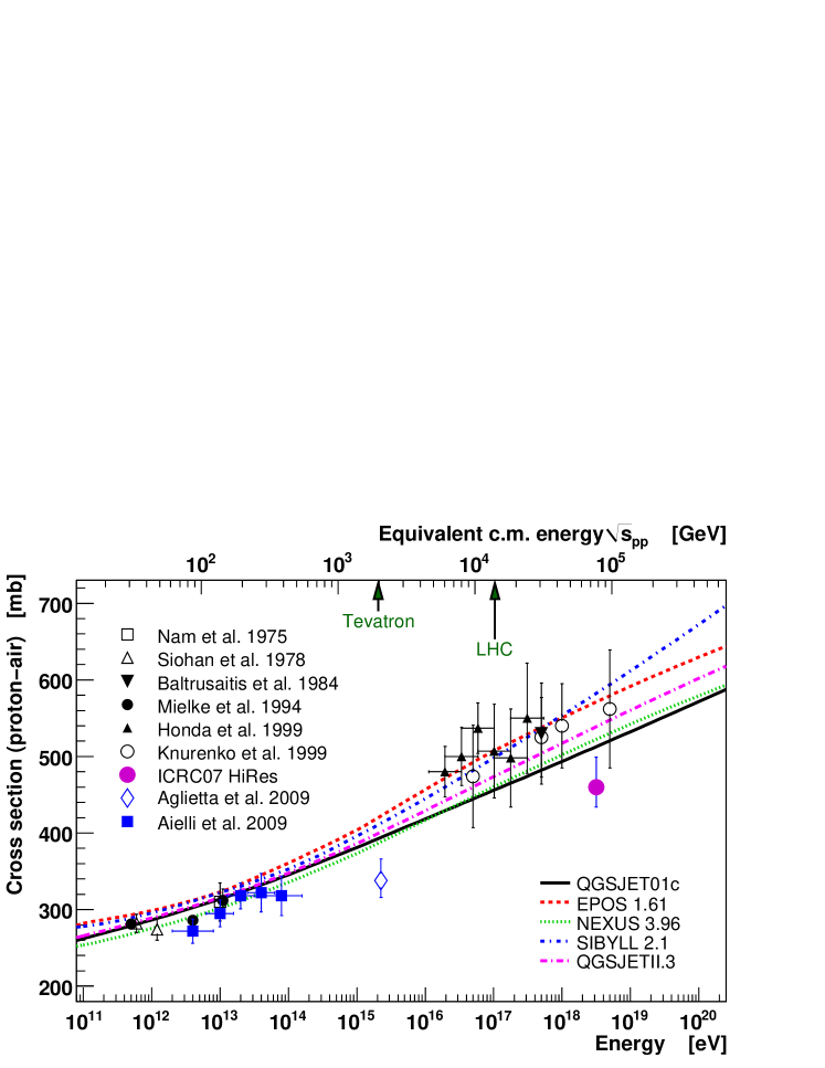
Figure 1: Compilation of proton-air production cross sections from cosmic ray measurements [2, 3, 4, 5, 6, 7, 8, 9, 10, 11, 12, 13, 14]. The data are compared to model predictions [16, 17, 18, 19, 20, 21].

A compilation of published proton-air cross section measurements and predictions of ultra-high energy hadronic interaction models is shown in Fig. 1. All data above 100 TeV are based on the analysis of EAS data [7, 8, 9, 10, 11, 12, 13]. Also the ARGO-YBJ measurements around 10 TeV are originating from a high altitude EAS array [14]. The data at lower energies stem from unaccompanied hadron analyses [2, 3, 4, 5, 6].

All cosmic ray measurements of the proton-air cross section are only sensitive to the particle production cross section [9, 22]. In addition, interactions with insignificant particle production have no measurable impact on cosmic ray observations. This is the case for air shower based techniques as well as for the unaccompanied hadron method.

To draw conclusions on the energy of the primary particle and its first ultra-high energy interactions, all relevant processes involved from the primary cosmic ray particle entering the atmosphere up to the measurement of the EAS observable need to be modeled as precisely as possible. Sophisticated EAS Monte Carlo simulation programs are available for this task. This results in a highly indirect analysis procedure.

In this article we will perform a detailed Monte Carlo study of different methods to derive the proton-air cross section from air shower data at an energy of $\sim 10^{19}\,\mathrm{eV}$. We will assume protons as cosmic ray particles in the energy range considered here. Although there exist theoretical models [23, 24, 25, 26, 27] and also experimental indications [28, 29, 30] for this flux being indeed dominated by protons, other elements in the primary flux have also to be taken into account. This will be done in a forthcoming article that will address specifically this topic [31].

Based on the results of the Monte Carlo study of existing analysis methods a general improvement is proposed and explicitly applied to one of the methods. By accounting for the actually measured cross section already in the simulation of showers, the systematic uncertainty due to the limited knowledge of hadronic interactions is significantly reduced. The performance of the improved method is thoroughly tested for the application to high quality data of the depth of the shower maximum. Sources of systematic uncertainties of the resulting cross section are discussed. It is shown that the dependence on the hadronic interaction model, the most important source of systematic uncertainties, can be significantly reduced by incorporating the measured cross section in a consistent way in the shower simulation.

The analyses of this work are done at an energy of $10^{19}\,\mathrm{eV}$, at which high statistics data are available or expected from HiRes [32], the Pierre Auger Observatory [33], and Telescope Array [34], but the results are qualitatively also valid at other energies. The expected reduction of the model dependence will be smaller at energies where data from accelerators are available, i.e. $10^{15}\,\mathrm{eV}$ and below.

2 Relation between air shower observables and depth of the first interaction point

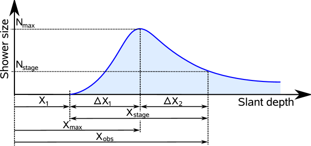
Figure 2: Definition of variables to characterize EAS longitudinal shower development. Zero slant depth is where the cosmic ray particle enters the atmosphere. The first interaction occurs at $X_{1}$. At $X_{\rm max}$ the shower reaches its maximum particle number $N_{\rm max}$. After the maximum the shower is attenuated over $\Delta X_{2}$ before it reaches the particle number $N_{\rm stage}$ at the slant depth of $X_{\rm obs}$.

Interactions over many decades in energy are occurring during EAS development. In the startup phase of the shower, relatively few ultra-high energy hadronic interactions are distributing the energy of the primary cosmic ray particle to a quickly growing number of secondary particles. The stochastic nature of these initial interactions is the source of strong fluctuations of EAS initiated by identical cosmic ray particles (shower-to-shower fluctuations). A significant part of secondary particles decay to electromagnetic particles and lead to the development of an electromagnetic cascade that, already after a few interactions, contains most of the total EAS energy and constitutes by far the largest fraction of the particles. The interactions of particles in the e.m. cascade are theoretically well understood. Also the large number of these interactions levels out additional large-scale fluctuations. Thus, the development of an air shower can be characterized by two main stages:

• Startup phase, consisting of few initial hadronic interactions at ultra-high energies. These interaction are the main source of fluctuations.

• Cascade phase, in which very numerous interactions of the bulk of the shower particles at intermediate energies take place. No significant large-scale fluctuations are expected from this part.

A clear boundary between the two stages cannot be drawn. The transition is seamless and by itself subject to strong shower-to-shower fluctuations. Only treatment with full air shower Monte Carlo simulation programs can fully account for all fluctuations.

To discuss the relation of the depth of the first interaction point to air shower observables it is useful to introduce a simple longitudinal model of air shower development that connects the proton-air cross section to the observables in a transparent way. The naming conventions for the model are given in Fig. 2. We distinguish between two types of air shower observation: by ground based detector arrays and the direct observation of longitudinal shower profiles by telescope detectors. The relevant air shower observables used in proton-air cross section analyses are the position of the shower maximum, $X_{\rm max}$, or the combination of the number of electrons $N_{\rm e}$ and muons $N_{\mu}$ at the atmospheric slant depth of the detector $X_{\rm obs}$.

In the following, the correlation of these EAS observables to the characteristics of the ultra-high energy interactions is studied with the one dimensional air shower Monte Carlo program CONEX v2r2 [38].

The particle numbers are defined as the total number of electrons above 1 MeV and muons above 1 GeV. This corresponds to typical quantities observed in air shower arrays, however the exact definition of observables depends very much on the experimental setup and varies strongly from experiment to experiment. By using the total number of particles for our study we are focusing on general air shower properties.

The shower maximum $X_{\rm max}$ is the slant depth of the maximum energy deposit of the shower in the atmosphere. This definition matches the shower maximum derived from the fluorescence light profile of showers and coincides with that of the particle number within $\sim 3\,\mathrm{gcm^{-2}}$.

2.1 Arrays of particle detectors

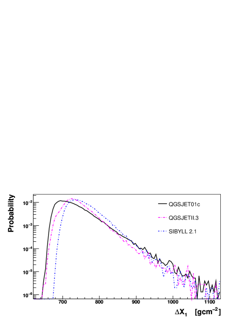
Figure 3: Distribution of the depth distance from the point of the first interaction up to the shower maximum for proton primaries at $10^{19}\,\mathrm{eV}$. The predictions of different models are compared.

Using ground based air shower arrays, one can estimate the proton-air cross section by measuring the frequency of air showers of the same energy and stage of their development at different atmospheric depths. By selecting events of the same energy but different directions of incidence, the point of the first interaction has to vary with the angle, in order to observe the shower at the same stage of development. The selection of showers of constant energy and stage can be done only approximately and depends on the particular detector setup, but the typical requirement is a constant $(N_{\rm e},N_{\mu})$ at observation level. Examples of measurements of this type are [7, 8, 10, 9, 14]. By requiring a given number of muons at the detector level does, in first approximation, select EAS of the same primary energy, because the attenuation of muons is small. However, also muons are slowly attenuated in the atmosphere. To correct for that a constant intensity selection can be applied [39]. Showers with identical primary energy at the same stage of their shower development are assumed to yield the same number of electrons since, after the shower maximum, the electromagnetic shower attenuation is approximately universal [40, 41, 42, 43, 44, 45].

The number of showers $N_{\rm sh}$ selected per area ${\rm d}A$ and time ${\rm d}t$, requiring a constant $(N_{e},N_{\mu})$ at the atmospheric depth $X_{\rm obs}$ can be written as

$$\frac{{\rm d}N_{\rm sh}}{{\rm d}N_{\rm e}\,{\rm d}N_{\mu}\,{\rm d}X_{\rm obs}\,{\rm d}A\,{\rm d}t} = \int{\rm d}\Omega\,{\rm d}E\,{\rm d}X_{1}\,{\rm d}\Delta X_{1}\,{\rm d}\Delta X_{2}\,\frac{{\rm e}^{-X_{\rm 1}/\lambda_{\rm int}}}{\lambda_{\rm int}}\,$$ (3)

$$\times P_{\Delta X_{1}}(E)~{}P_{\Delta X_{2}}(E,X_{1},\Delta X_{1})~{}P_{N_{\mu}}(E,X_{1},\Delta X_{1},\dots)$$

$$\times\delta\bigl{(}X_{\rm obs}-X_{1}-\Delta X_{1}-\Delta X_{2}\bigr{)}$$

$$\times\frac{{\rm d}N_{\rm CR}}{{\rm d}\Omega\,{\rm d}E\,{\rm d}A\,{\rm d}t\,}\;,$$

where ${\rm d}N_{\rm CR}/({\rm d}\Omega\,{\rm d}E\,{\rm d}A\,{\rm d}t)$ is the flux of cosmic ray particles. The distribution $P_{\Delta X_{1}}={\rm d}p_{1}/{\rm d}\Delta X_{1}$ describes shower-to-shower fluctuation of $\Delta X_{1}$, see Fig. 3. The two-dimensional probability density $P_{\Delta X_{2}}={\rm d}p_{2}/({\rm d}\Delta X_{2}\,{\rm d}N_{\rm e})$ is the frequency of showers of given energy $E$, $X_{1}$, and $\Delta X_{1}$ to have a shower size $N_{\rm e}$ at a depth distance $\Delta X_{2}$ from the shower maximum. It is required that the electron number after the shower maximum is attenuated to $N_{\rm e}$, while $X_{\rm obs}=X_{1}+\Delta X_{1}+\Delta X_{2}$. The selection of showers by energy according to their muon number is reflected by the energy dependent probability distribution $P_{N_{\mu}}={\rm d}p_{\mu}/{\rm d}N_{\mu}$.

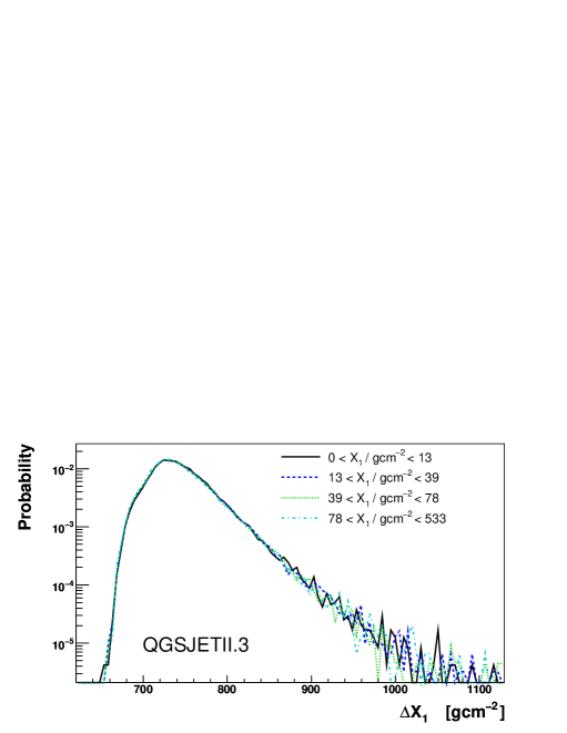
Figure 4: Independence of $P_{\Delta X_{1}}$ of $X_{\rm 1}$, demonstrated for primary protons at $10^{19}\,\mathrm{eV}$ with QGSJetII.

It is important to notice that the distribution $P_{\Delta X_{1}}$ does not depend on the depth $X_{1}$ of the first interaction point. This is shown in Fig. 4 for one hadronic interaction model. At high energy, and for air densities of relevance, almost all charged secondary pions always interact and all neutral pions decay immediately. Furthermore, the electromagnetic cascade initiated by the photons from $\pi^{0}$ decay does not depend on the local air density. This makes the startup phase of a shower to a good approximation independent of $X_{1}$.

The distribution $P_{\Delta X_{1}}$ depends, however, on the hadronic interaction model used for simulation. This is displayed in Fig. 3: both the mean $\Delta X_{1}$ and the shape of the distribution depend strongly on the chosen interaction model. In contrast, the distribution $P_{\Delta X_{2}}$ exhibits only a small model dependence due to the universality of electromagnetic air showers after shower maximum, see Fig. 5 (left).

An additional source of strong model dependence of Eq. (3) is the number of muons predicted for a given shower energy and depth. This can be seen in Fig. 5 (middle) where the frequency of finding a certain muon number for showers at $10^{19}$ eV and different models is shown. The effect of this model dependence is displayed in Fig. 5 (right) by showing the folded distributions

$$\left.P_{\rm eff}\right|_{N_{e},N_{\mu}}\propto\int P_{\Delta X_{2}}~{}P_{N_{\mu}}~{}E^{-3}~{}{\rm d}E\,.$$ (4)

In real data analysis it must be taken into account that $X_{\rm obs}$, $N_{\rm e}$ and $N_{\mu}$ are only known with a limited precision due to the detector and shower reconstruction resolution. In the model described by Eq. (3) this would furthermore add the corresponding uncertainty distributions $P_{\rm res}^{\rm S}$ and integrations over the three observables. The influence of the measurement resolution will be discussed below but is not included in (3) for sake of clarity.

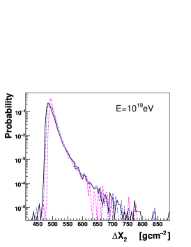
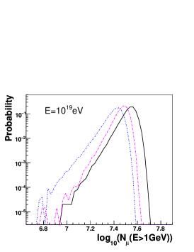
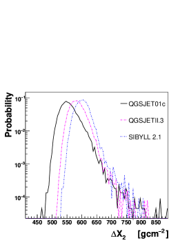
Figure 5: Model dependence of longitudinal air shower development for proton primaries. Left panel: Slant depth distance from the shower maximum up to the depth where showers are attenuated to $N_{\rm e}(E_{\rm e}>1\,\mathrm{MeV})=10^{9}$ electrons. Middle panel: Number of muons above 1 GeV after $1000\,\mathrm{gcm^{-2}}$ of shower development. Right panel: Same as left panel, but for showers selected according to $7.6<\log_{10}N_{\mu}(E_{\mu}>1\,\mathrm{GeV})<7.7$. While the plots on the left and in the middle are obtained from fixed energy simulations, the right plot is based on an energy spectrum $\propto E^{-3}$.

2.2 Optical telescopes

Using fluorescence telescopes, the distribution of $X_{\rm max}$ can be measured directly to obtain a handle on the value of the cross section at the highest energies [46, 47].

The direct observation of the position of the shower maximum allows us to simplify Eq. (3) by removing the term $P_{\Delta X_{2}}$ describing the shower development after the shower maximum and the distribution $P_{\mu}$ has to be replaced by a corresponding energy estimator based on the longitudinal shower profile. The resulting distribution of $X_{\rm max}$ can be written as

$$\frac{{\rm d}N_{\rm sh}}{{\rm d}X_{\rm max}{\rm d}E_{\rm em}{\rm d}A{\rm d}t} = \int{\rm d}\,\Omega\,{\rm d}E\,{\rm d}X_{\rm 1}\,{\rm d}\Delta X_{\rm 1}\;\frac{{\rm e}^{-X_{\rm 1}/\lambda_{\rm int}}}{\lambda_{\rm int}}\,P_{\Delta X_{1}}(E)\;P_{E_{\rm em}}\,$$ (5)

$$~{}~{}\times\delta\bigl{(}X_{1}+\Delta X_{1}-X_{\rm max}\bigr{)}\,\frac{{\rm d}N_{\rm CR}}{{\rm d}A\,{\rm d}t\,{\rm d}\Omega\,{\rm d}E}\;.$$

Here $E_{\rm em}$ denotes the electromagnetic, i.e. calorimetric energy of the shower that can be obtained from the integration of the energy deposit profile. There is a very good correlation between the primary energy and the calorimetric energy [48]. This correlation and the weak energy dependence of the depth of shower maximum allow us to neglect $P_{E_{\rm em}}={\rm d}p_{\rm em}/{\rm d}E_{\rm em}$ in our numerical studies.

3 Analysis of cross section measurement methods

The aim of all methods to measure the cross section is the determination of the interaction length $\lambda_{\rm int}$ from measured distributions that represent the l.h.s. of Eqs.(3,5).

3.1 “$k$-factor” techniques

The approximation of an exponential attenuation of the frequency of air showers after the penetration of large amounts of atmosphere is the basis of the $k$-factor method [7, 46, 47], which has been used to analyze both $X_{\rm max}$ and $(N_{\rm e},N_{\mu})$ data. The exponential slope of the attenuation is typically denoted by $\Lambda$, which is then related to the hadronic interaction length by a so-called $k$-factor

$$\Lambda=k\,\lambda_{\rm p-air}\;.$$ (6)

While this method has been applied to data of air shower arrays as well as telescope detectors [8, 9, 10, 7, 14, 12, 11], the definition of the $k$-factor for a ground array, $k_{\rm S}$, and for a telescope detector, $k_{\rm X}$, are not identical. Air shower fluctuations enter differently into $k_{\rm S}$ and $k_{\rm X}$ and the detector resolutions are also very different. This can be understood based on Eq. (3) and (5), which can both be approximated by exponential distributions for large $X_{\rm max}$, respectively $X_{\rm obs}$. For the $(N_{\rm e},N_{\mu})$ method this corresponds to

$$\left.\frac{{\rm d}N_{\rm sh}}{{\rm d}\sec\theta}\right|_{N_{\rm e},N_{\mu}}\;\propto\;{\rm e}^{-X_{\rm obs}/\Lambda_{\rm S}}\;\propto\;{\rm e}^{-X_{\rm obs}^{\rm vert}\sec\theta/\Lambda_{\rm S}}\;,$$ (7)

while for the $X_{\rm max}$-tail method it is

$$\frac{{\rm d}N_{\rm sh}}{{\rm d}X_{\rm max}}\;\propto\;{\rm e}^{-X_{\rm max}/\Lambda_{\rm X}}\;.$$ (8)

This assumes that there are no significant non-exponential contributions to the tails of the distributions, which is not true in general as it will be shown in the following. Since the full distributions are described by Eq. (3) and (5) it is possible to calculate the tails based on the given convolution integrals. Each of the integrations will give a contribution, so for $(N_{\rm e},N_{\mu})$ one gets

$$\Lambda_{\rm S}=\lambda_{\rm int}\,k_{\Delta X_{\rm 1}}\,k_{\Delta X_{\rm 2}}\,k_{\rm res}^{\rm S}=\lambda_{\rm int}\,k_{\rm S}\qquad\mbox{with}\qquad k_{\rm S}=k_{\Delta X_{\rm 1}}\,k_{\Delta X_{\rm 2}}\,k_{\rm res}^{\rm S}\;,$$ (9)

while for $X_{\rm max}$-tail just

$$\Lambda_{\rm obs}^{\rm X}=\lambda_{\rm int}\,k_{\Delta X_{\rm 1}}\,k_{\rm res}^{\rm X}=\lambda_{\rm int}\,k_{\rm X}\qquad\qquad\mbox{with}\qquad k_{\rm X}=k_{\Delta X_{\rm 1}}\,k_{\rm res}^{\rm X}\,,$$ (10)

where $\lambda_{\rm int}$ is the proton-air interaction length, $k_{\Delta X_{1}}$ the contribution from the integration of $P_{\Delta X_{1}}$, $k_{\Delta X_{2}}$ the one from $P_{\Delta X_{2}}$ and $k_{\rm res}^{\rm S/X}$ the part due to the detector resolution. The individual contributions of $k_{\Delta X_{1}}$, $k_{\Delta X_{2}}$ and $k_{\rm res}^{\rm S/X}$ are difficult to compute and not known in most of the existing analyses, except the one in Ref. [12] and even more complete in Ref. [14].

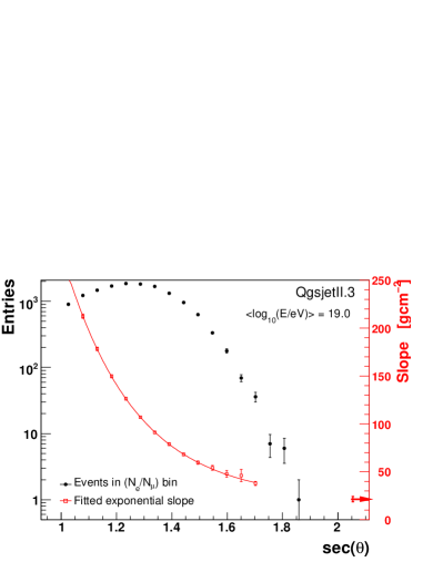
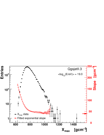
Figure 6: Left panel: $(N_{\rm e},N_{\mu})$-method. Right panel: $X_{\rm max}$-tail method. The fitted open symbols show the dependence of the resulting exponential slope on the choice of the begin of the fit range. The arrow indicates the asymptotic behavior of the fit, deduced from Eq. (11), and its statistical uncertainty.

For a given experimental setup and analysis approach it is possible to estimate the values of $k_{\Delta X_{1}}$, $k_{\Delta X_{2}}$, $k_{\rm res}^{\rm X}$ and $k_{\rm res}^{\rm S}$ as well as their dependence on hadronic interaction models. This is demonstrated here for an artificial experimental setup as described below. For each of the hadronic interaction models QGSJet01c, QGSJetII.3 and SIBYLL 2.1 a set of $\sim 400,000$ proton induced air showers is simulated with a primary energy distribution ${\propto}E^{-3}$ between $18.7<\log_{10}E/\rm eV<19.4$ and a zenith angle distribution of ${\rm d}N\propto\cos\theta\,{\rm d}\cos\theta$. Two histograms are produced and analyzed for every set of simulations:

• Distribution of $X_{\rm max}$ with $18.9<\log_{10}E/\rm eV<19.15$. A Gaussian detector resolution with $\sigma(X_{\rm max})=20\,\mathrm{gcm^{-2}}$ and an energy resolution of $\sigma(E)/E=0.1$ is assumed, which corresponds to values reported by the Pierre Auger Collaboration [49]. The resulting mean energy of this data sample is $10^{19.0}\,\mathrm{eV}$.

• Distribution of events with $1.26<N_{\rm e}/10^{9}<3.98$ and $0.28<N_{\mu}/10^{8}<1.12$ at a vertical atmospheric depth of $X_{\rm obs}^{\rm vert}=860\,\mathrm{gcm^{-2}}$ (corresponding to the Pierre Auger Observatory) versus $\sec\theta$. The $N_{\rm e}$ cut selects showers past their maximum ($N_{\rm e}^{\rm max}(10^{19}\,\mathrm{eV})\sim 6.3\cdot 10^{9}$) as done, for example, in the pioneering Akeno analysis [7]. The detection resolution of $N_{\rm e}$ and $N_{\mu}$ are assumed to be Log-Normal with a resolution of $\sigma(\log_{10}N_{\rm e})/\log_{10}N_{\rm e}=0.05$ and $\sigma(\log_{10}N_{\mu})/\log_{10}N_{\mu}=0.1$ as well as the zenith angle uncertainty of $\sigma(\theta)=1.0^{\circ}$. Due to significant model-differences in the prediction of muon numbers the selected data samples have slightly differing energies (from $10^{18.96}\,\mathrm{eV}$ for QGSJet01 up to $10^{19.04}\,\mathrm{eV}$ for SIBYLL).

The histograms are fitted with an exponential function by a log-likelihood fit, which allows to correctly include empty bins in the analysis. The fit range is chosen as follows: While the end of the fit, $X^{\rm fit}_{\rm end}$, is always $50\,\mathrm{gcm^{-2}}$ beyond the last non-zero entry in the histogram, the start of the fit, $X^{\rm fit}_{\rm start}$, is varied. The resulting dependence of the exponential slopes on the start of the fitting range is then parameterized by

$$\Lambda(X^{\rm fit}_{\rm start})=\Lambda_{0}+\Lambda_{1}\,{\rm e}^{-c\,X^{\rm fit}_{\rm start}}\;,$$ (11)

where the asymptotic slope $\Lambda_{0}$ for $X^{\rm fit}_{\rm start}\rightarrow\infty$ is taken to be the fit range-independent value of the exponential slope. In Fig. 6 this procedure is displayed for histograms obtained with the QGSJetII interaction model. It is found that the choice of the fit range has a major impact on the outcome of the slope. This is consistent with the results of [39]. For the ($N_{\rm e}$,$N_{\mu}$)-method, generally no plateau is found and the resulting value for $\Lambda_{0}$ is highly unstable. Thus, it is hardly possible to define a meaningful slope of the tail for this case. The situation for $X_{\rm max}$ is somewhat better. While a stable plateau is still difficult to identify, $\Lambda_{0}$ can be estimated reliably. With this analysis approach the resulting asymptotic values, $\Lambda_{0}$, are slightly lower than the values obtained for $\Lambda$ directly from fits to the distributions. So neither the slopes nor the $k$-factors can be directly compared to results from previous analyses. Nevertheless, the found model dependence and other methodical problems will apply in a similar way to previous analyses. The strong dependence of the slope on the chosen fitting range is a severe methodical problem of the $k$-factor technique. Without a given method to infer a meaningful slope from such distributions, as for example the one proposed here, the $k$-factor technique cannot produce reliable results.

The obtained slopes $\Lambda_{0}$ are then compared to the interaction mean free path length of the primary particle in the atmosphere, $\lambda_{\rm p-air}$, of the interaction model used in the CONEX simulations. In Tab. 1 the resulting $k$-factors are listed together with their propagated statistical uncertainties. The total model induced uncertainties on the $k_{\rm S/X}$-factors are $\sim 7\,\mathrm{\%}$ for the $X_{\rm max}$-tail and $\sim 28\,\mathrm{\%}$ for the $(N_{\rm e},N_{\mu})$-method. Looking to the $k$-factor components one can see that a part of the model induced uncertainty enters already in the shower development up to the shower maximum ($k_{\Delta X_{1}}$), while the shower development after the shower maximum ($k_{\Delta X_{2}}$) adds the more significant amount of model-dependence. Another large contribution comes from $k_{\rm res}^{\rm S}$, which is mostly related to very differing model predictions on the number of muons. The factor $k_{\rm res}^{\rm X}$ is only marginally model-dependent, which is originating from the very small model differences in the energy dependence of $X_{\rm max}$.

While this study mostly serves illustrative purposes, and the chosen experimental and analysis parameters are arbitrary, it nevertheless demonstrates the impact of model dependence on $k$-factor techniques. The found model dependence is rooted in the underlying air shower physics as well as in typical detector characteristics.

Table 1: Resulting $k$-factors from CONEX study for primary protons at $10^{19}\,\mathrm{eV}$. In each column the maximal and minimal $k$-factors are highlighted. The difference between those maxima is denoted by $\Delta$ and is a measure of model-dependence.

Model	$k_{\Delta X_{1}}$	$k_{\Delta X_{2}}$	$k_{\rm res}^{\rm X}$	$k_{\rm res}^{\rm S}$	$k_{\rm X}$	$k_{\rm S}$
QgsjetII.3	1.00$\pm$0.01	0.61$\pm$0.06	0.92$\pm$0.01	0.81$\pm$0.10	0.92$\pm$0.01	0.49$\pm$0.06
Qgsjet01c	1.14$\pm$0.00	0.48$\pm$0.05	0.93$\pm$0.01	0.50$\pm$0.14	1.06$\pm$0.01	0.27$\pm$0.08
Sibyll 2.1	1.02$\pm$0.00	0.68$\pm$0.06	0.93$\pm$0.01	0.61$\pm$0.11	0.94$\pm$0.01	0.42$\pm$0.08
Mean	1.05$\pm$0.00	0.59$\pm$0.03	0.92$\pm$0.00	0.64$\pm$0.07	0.97$\pm$0.00	0.40$\pm$0.04
$\Delta$	0.07$\pm$0.00	0.10$\pm$0.04	0.01$\pm$0.00	0.16$\pm$0.09	0.07$\pm$0.00	0.11$\pm$0.05

3.2 Unfolding of the $X_{\rm max}$-distribution

An improvement of the cross section measurement techniques is achieved by explicitly accounting for air shower fluctuations [13]. This allows one to use not only the slope but also the shape of the $X_{\rm max}$-distribution. The measured $X_{\rm max}$-distribution, Eq. (5), is unfolded using a given $P_{\Delta X_{\rm 1}}$-distribution to retrieve the original $X_{\rm 1}$-distribution. Of course, the $\Delta X_{1}$-distribution needs to be inferred from simulations, which ultimately introduces a comparable model dependence as in the $k$-factor techniques [50]. The model dependence of the most important part of the kernel function, $P_{\Delta X_{1}}$, can be seen in Fig. 3.

In the unfolding technique, a larger range of the $X_{\rm max}$-distribution is used. If the primary particles are known to be protons only, a cross section analysis can be done already with very limited shower statistics. On the other hand, the results of this method are more sensitive to a possible fraction of primary particles that are not protons.

4 An improved method to derive the proton-air cross section

One of the shortcomings of cross section analysis methods applied so far is the missing connection between the cross section of the first interaction, that is to be measured, and the cross sections used in the calculation of the various probability distributions in Eqs. (3) and (5).

In the following we consider the method of unfolding the $X_{\rm max}$ distribution, applicable to fluorescence telescope measurements, and improve it by consistently accounting for the “measured” high-energy cross section. We will calculate the full shape of the distribution of $X_{\rm max}$, depending only on properties of hadronic interactions at ultra-high energies. The impact of changing features of hadronic interactions at ultra-high energies on the longitudinal air shower development, i.e. $P_{\Delta X_{1}}$, is parameterized and used within the calculation. It is straightforward to refine the modeling by incorporating detector acceptance as well as the energy distribution of analyzed data.

4.1 Description of the $X_{\rm max}$-distribution

The description of the distribution of observed $X_{\rm max}^{\rm rec}$ in terms of $\sigma_{\rm p-air}$ is based on Eq. (5), now written with the term for the experimental $X_{\rm max}$ resolution

$$\frac{{\rm d}N_{\rm sh}}{{\rm d}X_{\rm max}^{\rm rec}}\propto\int{\rm d}X_{\rm 1}\,{\rm d}\Delta X_{\rm 1}\, \,{\rm d}X_{\rm max}\;\;\frac{{\rm e}^{-X_{\rm 1}/\lambda_{\rm int}}}{\lambda_{\rm int}}\;P_{\Delta X_{1}}(E,\lambda_{\rm int},\Delta X_{1}+X_{\rm shift})$$ (12)

$$\times\,\delta(X_{1}+\Delta X_{1}-X_{\rm max})\;P_{\rm res}^{\rm X}\bigl{(}X_{\rm max}^{\rm rec}\,|\,X_{\rm max}\bigr{)}\;.$$

The parameter $X_{\rm shift}$ allows us to shift the $P_{\Delta X_{1}}$-distribution by replacing $\Delta X_{\rm 1}$ with $\Delta X_{\rm 1}+X_{\rm shift}$. The introduction of the $X_{\rm shift}$ parameter is necessary in order to reduce the model dependence of the analysis [50]. This can be easily understood by looking at the $P_{\Delta X_{1}}$-distributions shown in Fig. 3, which appear to be shifted between different models by up to $\sim 60\,\mathrm{gcm^{-2}}$. It is found that the $X_{\rm shift}$ parameter is highly model dependent and comprises many additional effects of the characteristics of high energy hadronic interactions on the $X_{\rm max}$-distribution. It can be demonstrated that differences between the inelasticity or the secondary multiplicity of the models may act as a cause for such an additional shift [51]. The only important assumption related to the role of $X_{\rm shift}$ in the cross section analysis is that any additional and unknown changing characteristics of hadronic interactions at extreme energies contributes mainly to a global shift of $X_{\rm max}$ and thus $\Delta X_{\rm 1}$, while leaving the shape of the distributions unchanged.

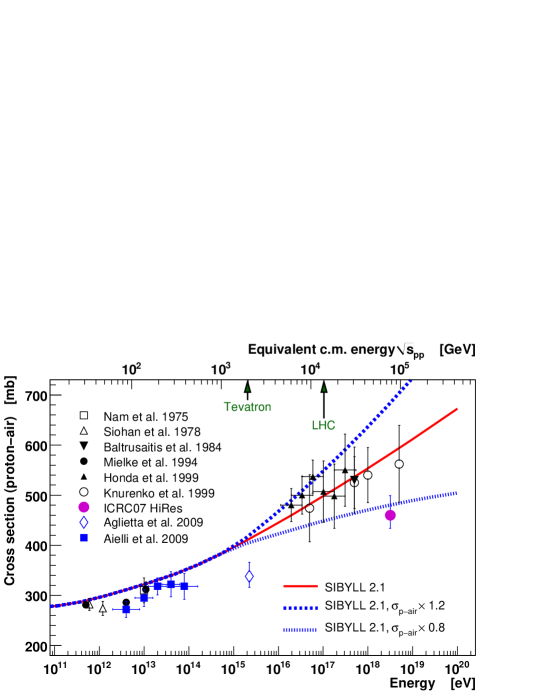
Figure 7: Modified extrapolation of the proton-air cross section. Shown are the original prediction from SIBYLL together with a $20\,\mathrm{\%}$ increased respectively decreased cross section at $10^{19}\,\mathrm{eV}$.

The cross section analysis proceeds then as follows. The $X^{\rm rec}_{\rm max}$-distribution is calculated from Eq. (12) for a given interaction length $\lambda_{\rm int}$ and shift parameter $X_{\rm shift}$ and compared to the measured distribution. By performing a log-likelihood fit with the interaction length and an overall shift in depth as free parameters, the cross section and the $1\sigma$ uncertainty band is found [50].

One major improvement with respect to previous cross section analysis approaches is the consideration of the impact of a changing cross section on the resulting shower development described by $P_{\Delta X_{1}}$. It is assumed that the cross section is reasonably well known at the energy corresponding to that of the Tevatron collider. Starting from this energy of $\sim 2\times 10^{15}$ eV, cross sections of the model used for the calculation of $P_{\Delta X_{1}}$ are rescaled by a factor $f(E)$ that increases logarithmically with energy and ensures that the modified model cross section matches the corresponding value of the fit parameter $\lambda_{\rm int}$ at the considered shower energy. Here we will use $10^{19}$ eV as reference for the scaling parameter being $f_{19}$ at this energy. Then the scaling factor reads

$$f(E)=1+(f_{19}-1)\frac{\ln(E/10^{15}\,{\rm eV})}{\ln(10^{19}\,{\rm eV}/10^{15}\,{\rm eV})},$$ (13)

for $E>10^{15}$ eV and $f(E)=1$ otherwise. The idea of the rescaling of the cross section is shown in Fig. 7, where the proton-air cross section of SIBYLL is shown together with cross sections that are scaled up and down by 20 % at $10^{19}$ eV.

So far the dependence of $P_{\Delta X_{1}}$ on the cross section has been neglected in air shower based cross section measurement. In fact, any attempt to determine the proton-air cross section without taking this dependence into account is overestimating the impact of $\sigma_{\rm p-air}$ on the analyzed observables since part of the measured effect must be attributed to a modified development of the air shower and not to the fluctuations of the first interaction point.

To implement the idea of modified cross sections in the data analysis one needs to parameterize the $\Delta X_{1}$-distribution and determine its energy dependence and the modification of this distribution as function of the cross section scaling parameter. This is done using a Moyal distribution extended by one parameter and described in detail in A. In Fig. 8 example $\Delta X_{1}$-distributions are shown together with fits of the extended Moyal distribution and also the final parameterizations.

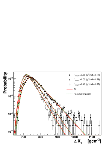
(a) QGSJetII.3

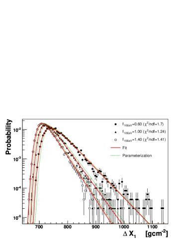
(b) SIBYLL 2.1

Figure 8: Simulated $\Delta X_{\rm 1}$-distributions at $10^{19}\,$eV for two hadronic interaction models. Included are the fits of the extended Moyal distribution Eq. (14) as well as the final parameterization.

4.2 Fitting range and stability

To investigate the sensitivity of the method to the choice of the $X_{\rm max}$-range used for the fit, we generate sets of 3000 simulated data showers and analyzes them with Eq. (12). The Gaussian detector resolution for $X_{\rm max}$ is chosen to be 20 gcm^-2, which is the value reported by the Pierre Auger Collaboration [49].

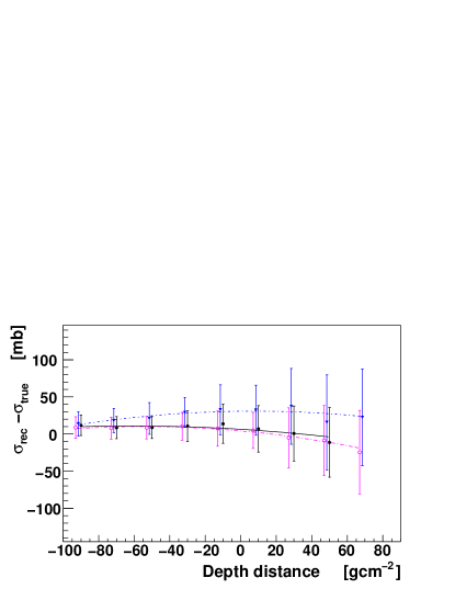
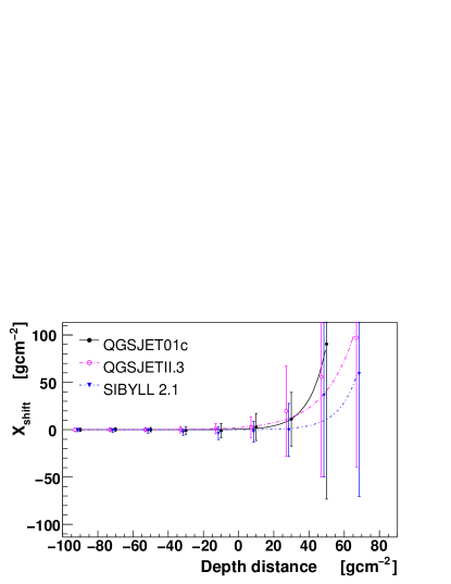
(a) Start of the fitting range, $X_{\rm max}^{\rm start}$ (relative to the peak of the $X_{\rm max}$-distribution)

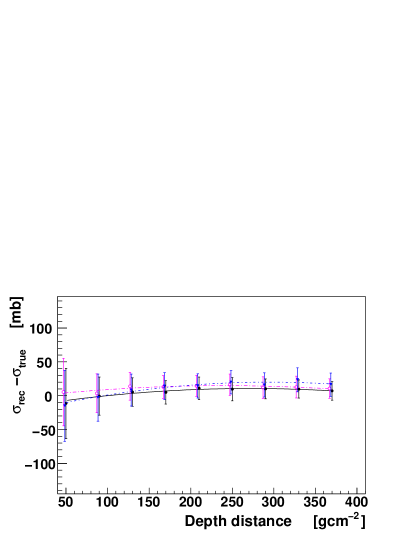
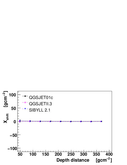
(b) End of the fitting range, $X_{\rm max}^{\rm stop}$ (relative to the peak of the $X_{\rm max}$-distribution)

Figure 9: Impact of the chosen fitting range in $X_{\rm max}^{\rm rec}$ on the resulting cross section (left) and $X_{\rm shift}$ (right) at $10^{19}\,\mathrm{eV}$. Each point corresponds to the mean of 100 reconstructions and the error bars denote the resulting RMS. Both, the reconstructed $X_{\rm max}$ as well as the $\Delta X_{1}$-distribution are produced independently with the specified interaction model. The lines are just to guide the eye.

The interval of the $X_{\rm max}$-distribution used to fit the model is important for the resulting statistical as well as systematical uncertainties. The first aspect is obvious since a reduction of the dataset is clearly leading to a reduced statistical power of the reconstruction. The latter one is mostly because of the possible contamination of the $X_{\rm max}$-distribution by cosmic ray primaries other than protons. All primary nuclei heavier than protons are producing shallower $X_{\rm max}$ compared to protons. Primary photons, on the other hand, are deeply penetrating and have a larger $X_{\rm max}$ than protons. A restricted fitting range in $X_{\rm max}$ can thus be used to enrich the considered fraction of protons and reduce a possible contamination by other cosmic ray primaries.

The resulting impact of the chosen fitting range on the performance of the reconstruction is shown in Figure 9. The position of the peak of the $X_{\rm max}$-distribution, $X_{\rm peak}$, is used as a reference to define the fitting range. The starting point as well as the ending point of the fit are expressed only relative to $X_{\rm peak}$.

Evidently, it is beneficial to chose the fitting range as large as possible to get the smallest resulting statistical uncertainties. It is possible to shift the beginning of the fitting range relatively close to $X_{\rm peak}$ without loosing too much statistical power (cf. Figure 9 (a)). It is found that, with the used parameterizations, the beginning of the fitting range can be set to 50 gcm^-2 in front of $X_{\rm peak}$. In the following this is the adopted default choice.

The choice of the end of the fitting range has a similar impact on the reconstruction. In Figure 9 (b) it is shown how the reconstruction is degrading, while choosing a shorter fitting range. Since the photon fraction of ultra-high energy cosmic ray primaries is already strongly constrained [52] there is no special need to restrict the upper end of the fitting range. In the following the upper end of the fitting range for the log-likelihood fit of the $X_{\rm max}$-distribution is set to the value of the maximum $X_{\rm max}$ plus 40 gcm^-2.

The cross section dependent parameterizations of the $\Delta X_{1}$-distributions are introducing a slight systematic overestimation of the reconstructed cross sections of $10-20\,\mathrm{mb}$, corresponding to $<5\%$. This can be taken into account within the determination of the total systematic uncertainties of the measurement. The statistical resolution of the reconstruction is around $20\,\mathrm{mb}$ for 3000 events.

5 Comparison of the performance of different analysis methods

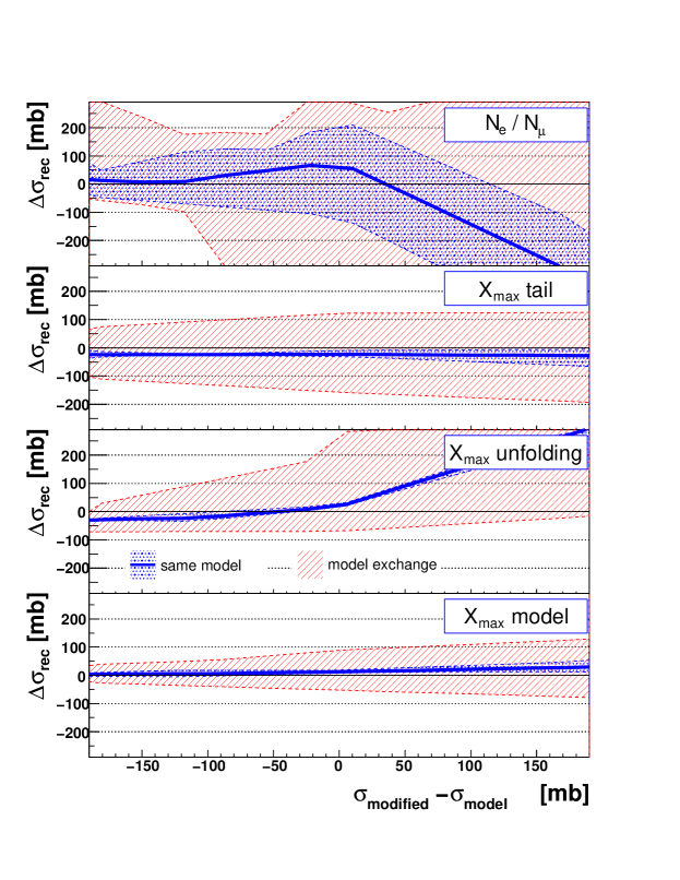
Figure 10: Resulting systematics and dependence on models of cross section reconstruction techniques. Every analysis was performed 100 times on 3000 simulated EAS; Shown are the mean results. The central shaded area shows the ability of a method to reconstruct the input cross section of simulated air shower data with the same model that was used for the simulations. The thick line marks the mean result for all used models, which are QGSJet01c, QGSJetII.3 and SIBYLL2.1. The width of the central band is caused by statistical fluctuations. The outer shaded area denotes the maximum deviation of the cross section reconstructed with a model that differs from the one used to generated the simulated dataset.

In order to test the ability of a reconstruction method to recover a changing input cross section, air shower simulations with a modified cross section (cf. A.2) are performed. The simulated air shower data are then reconstructed and the found cross sections $\sigma_{\rm rec}$ are compared to the modified input cross sections $\sigma_{\rm modified}=f_{19}\,\sigma_{\rm model}$. The result of this analysis for all cross section reconstruction methods is summarized in Fig. 10. The central shaded area together with the solid line demonstrates the principal self-consistency of the analysis technique. The outer shaded area can be interpreted as the maximum possible model-dependence of the reconstruction method.

With the $(N_{\rm e},N_{\mu})$-method it is very difficult to reconstruct a modified cross section. Additionally the model dependence of the result is generally large. It is difficult to quantify, but can easily be of the order of hundreds of mb.

A very much better performance is achieved by the $X_{\rm max}$-tail analysis. The deviation of the reconstruction cross section from the input value is not getting larger than $50\,\mathrm{mb}$ and the model-dependence is between $100-200\,\mathrm{mb}$.

The $X_{\rm max}$-unfolding technique can find cross sections that are not deviating much from the original model value. However, it shows a clear systematic trend of underestimating small cross sections and strongly overestimating large cross sections. Also the model dependence is not negligible, ranging from $\sim 75\,\mathrm{mb}$ at very low cross sections, $\sim 200\,\mathrm{mb}$ at intermediate cross sections to many hundreds of mb at large cross sections.

Finally, the $X_{\rm max}$-model demonstrates its unique ability to retrieve very consistently modified cross sections over a wide range. The model dependence is smaller than for the $X_{\rm max}$-tail method and is $<50\,\mathrm{mb}$ at low cross section while it grows to $\sim 100\,\mathrm{mb}$ at large cross sections.

The generally better sensitivity to reconstruct smaller compared to larger cross section is resulting from the increasing importance of the fluctuations of $X_{1}$ for the final $X_{\rm max}$-distribution. This facilitates the measurement of a small cross section, while for large cross sections $X_{\rm max}$-distributions are mostly shaped by fluctuations of the shower development $P_{\Delta X_{1}}$ and the detector resolution, making a measurement of the cross section generally more difficult.

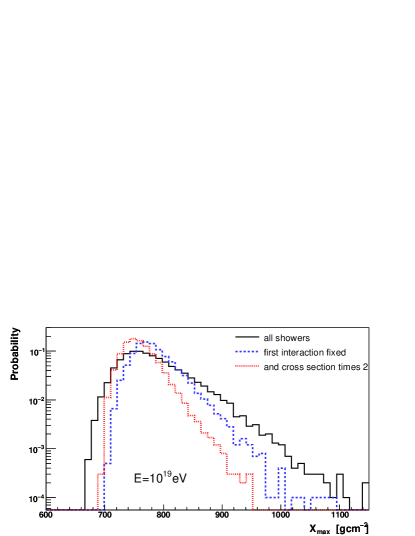
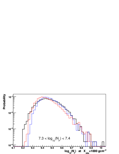
Figure 11: Shower-to-shower fluctuations of $X_{\rm max}$ (left) and $\log_{10}N_{\rm e}$ (right) for primary protons. The solid line is the original model prediction of QGSJetII, while the dashed line is for showers having their first interaction at the fixed slant depth corresponding to the predicted proton-air interaction length of QGSJetII. The dotted line is for simulated air showers with increased cross section by a factor of two, $f_{19}=2$, in addition to the fixed first interaction point.

Due to the combined impact of the fluctuation of both electron as well as muon numbers, the remaining sensitivity of the $(N_{\rm e},N_{\mu})$-method to the proton-air cross section is very much reduced compared to methods using the observable $X_{\rm max}$, see Fig. 11.

It is not straightforward to quantify the systematic effect caused by interaction models on the results of the proton-air cross section analyses. While the magnitude of the outer uncertainty band in Fig. 10 suggests relatively large model dependence of the results, this just reflects the existing incompatibility of the underlying models. Thus, it cannot be used to make any conclusion on the comparison of real data to the different models. For the analysis of real data, model dependence should be evaluated by the independent reconstruction of the data based on all available interaction models, and subsequent quoting of the mean result. The interval spanned by the reconstructions can then be used as an estimation of the systematic uncertainty induced by the models. This results in a smaller dependence on interaction models compared to Fig. 10.

6 Summary

It is demonstrated in methodical studies that all techniques to determine the proton-air cross section from air shower data are in fact based on the same fundamental formulation that describes the longitudinal air shower development. The requirement of using air shower Monte Carlo simulations to interpret EAS observables inevitably introduces a dependence on the hadronic interaction models used for the simulations.

It is found that the magnitude of the model dependence is similar for all cross section reconstruction methods; Only the $(N_{\rm e},N_{\mu})$-technique exhibits a significantly larger model dependence, which is due to the additional strong model dependence on the prediction of muon numbers. In addition, since the prediction of electron and muon numbers are both depending on interaction models, it is not possible to define model independent cuts for the selection of air shower events. Thus, already on the level of event selection, a model dependence is introduced in $(N_{\rm e},N_{\mu})$-analyses.

All $k$-factor based techniques are suffering from non-exponential contributions to the slope of the $X_{\rm max}$- respectively $(N_{\rm e},N_{\mu})$ frequency-distribution at large depths. Thus the exponential approximation used to define $k$-factors, is only of limited accuracy. Any non-exponential contribution creates a strong dependence of the exponential slope on the chosen fitting range (see also Ref. [53]).

Generally, $k$-factors are depending on the resolution of the experiment and can therefore not be simply transferred from one experiment to another, as done in some recent analysis [54]. In particular, $k_{\rm X}$-factors are inherently different from $k_{\rm S}$-factors and can therefore not be transferred from an $X_{\rm max}$-tail analysis to that of ground based frequency attenuation or vice versa.

An $X_{\rm max}$-based analysis technique, as proposed in Ref. [13], was further improved to reduce methodical and model induced systematic uncertainties on the cross section result as much as possible. The presented improved method is a model of the $X_{\rm max}$-distribution based on simple considerations on longitudinal air shower development combined with the parameterized impact of a changing cross section on the resulting air shower development. Previous reconstruction techniques assume a static $\Delta X_{1}$-distribution or $k$-factor, independent of the modified cross section. As, in general, the reconstructed cross section deviates from the predicted value of the hadronic interaction model used to generate the $\Delta X_{1}$-distribution or $k$-factor, a discrepancy of the data with the air shower simulations is inevitable. The data can not be described by the models used for the air shower simulations and it is not sufficient to adopt the measured cross section just for the first interaction point, while keeping the rest of the shower simulations unchanged.

For the case of a proton-dominated cosmic ray data sample around $10^{19}\,\mathrm{eV}$, which was studied in this article, it is possible to determine the proton-air cross section with good precision. The statistical uncertainties of the analysis of samples with 3000 events are about 20 mb (5 %) and the systematic uncertainties introduced by the parameterizations of the $X_{\rm max}$-model are of the same order of magnitude. The model-induced systematic uncertainty is between 50 and 100 mb, corresponding to relative uncertainties of $<10\,\mathrm{\%}$ to $\sim 20\,\mathrm{\%}$. A further reduction of this model-related uncertainty is possible, but needs improvements in the understanding of the underlying hadronic interaction physics.

Furthermore, the second free parameter of the new analysis technique, $X_{\rm shift}$, is a further handle that is sensitive to the physics of hadronic interactions at ultra-high energies. A non-zero result of $X_{\rm shift}$ indicates the deficiency of the underlying hadronic interaction model to describe the measured data distribution. It can be interpreted in terms of a modified characteristics of secondary particle production in hadronic interactions [51].

Appendix A Parameterization of $\Delta X_{\rm 1}$-distribution

A modified version of the Moyal distribution is introduced to parameterize the $\Delta X_{\rm 1}$-distribution

$$p_{\rm 1}(\Delta X_{\rm 1})=\frac{N}{\beta\,\sqrt{2\pi}}\;e^{-\frac{1}{2}\left(z+e^{-z\;\left(z^{2}\right)^{\gamma}}\right)}\qquad\mbox{with}\qquad z=\frac{\Delta X_{\rm 1}-\alpha}{\beta}\,.$$ (14)

The additional third degree of freedom $\gamma$ makes the parameterization more flexible, allowing us to improve the description around the peak of the $\Delta X_{\rm 1}$-distributions. The normalization value $N$ is not a free parameter, but is numerically computed to correctly normalize the distribution. Since the Moyal function with the two parameters $\alpha$ and $\beta$ itself is normalized, we only have to correct for the $\gamma$ parameter

$$N(\gamma)=\frac{1}{0.965+3.685\times 10^{-3}\;\bigl{(}\gamma+0.366\bigr{)}^{-2.171}}\,.$$ (15)

A.1 Energy dependence

To determine the energy dependence of the parameters $\alpha$, $\beta$ and $\gamma$, the parameterization Eq. (14) is fitted to $\Delta X_{\rm 1}$-distributions generated by CONEX at several primary energies. The energy dependence can then be interpolated by a polynomial of 2^nd degree

$$\alpha^{\rm e}(E) =\alpha_{0}^{\rm e}+\alpha_{1}^{\rm e}\;\log_{\rm 10}(E/\mbox{eV})+\alpha_{2}^{\rm e}\;\log_{\rm 10}^{2}(E/\mbox{eV})$$

$$\beta^{\rm e}(E) =\beta_{0}^{\rm e}+\beta_{1}^{\rm e}\;\log_{\rm 10}(E/\mbox{eV})+\beta_{2}^{\rm e}\;\log_{\rm 10}^{2}(E/\mbox{eV})$$ (16)

$$\gamma^{\rm e}(E) =\gamma_{0}^{\rm e}+\gamma_{1}^{\rm e}\;\log_{\rm 10}(E/\mbox{eV})+\gamma_{2}^{\rm e}\;\log_{\rm 10}^{2}(E/\mbox{eV})\,.$$

Table 2: Parameters for describing the energy dependence of $\Delta X_{1}$-distributions.

Model	Index $i$	$\alpha^{\rm e}_{i}$ [g/cm]		$\beta^{\rm e}_{i}$ [g/cm]		$\gamma^{\rm e}_{i}$ [1]
QGSJet01c	$0$	-871.25$\pm$	27.76	85.15$\pm$	14.49	5.94${\pm}$	1.43
	$1$	113.91$\pm$	3.01	-7.49$\pm$	1.57	-0.71${\pm}$	0.16
	$2$	-1.64$\pm$	0.08	0.22$\pm$	0.04	0.02${\pm}$	0.00
QGSJetII.3	$0$	-1320.67$\pm$	24.86	226.24$\pm$	11.68	6.04${\pm}$	0.39
	$1$	165.29$\pm$	2.70	-22.31$\pm$	1.27	-0.63${\pm}$	0.04
	$2$	-3.04$\pm$	0.07	0.59$\pm$	0.03	0.02${\pm}$	0.00
SIBYLL 2.1	$0$	-606.32$\pm$	20.37	131.27$\pm$	9.56	0.33${\pm}$	0.43
	$1$	79.17$\pm$	2.20	-11.78$\pm$	1.03	-0.05${\pm}$	0.05
	$2$	-0.45$\pm$	0.06	0.30$\pm$	0.03	0.00${\pm}$	0.00

The chosen polynomial interpolation is well suited to reproduce the found dependences over the considered energy range. The results are illustrated in Fig. 12 and the parameters are listed in Table 2. A first result is that even the energy dependence of $\Delta X_{\rm 1}$ is depending on the high energy interaction model used during air shower simulations.

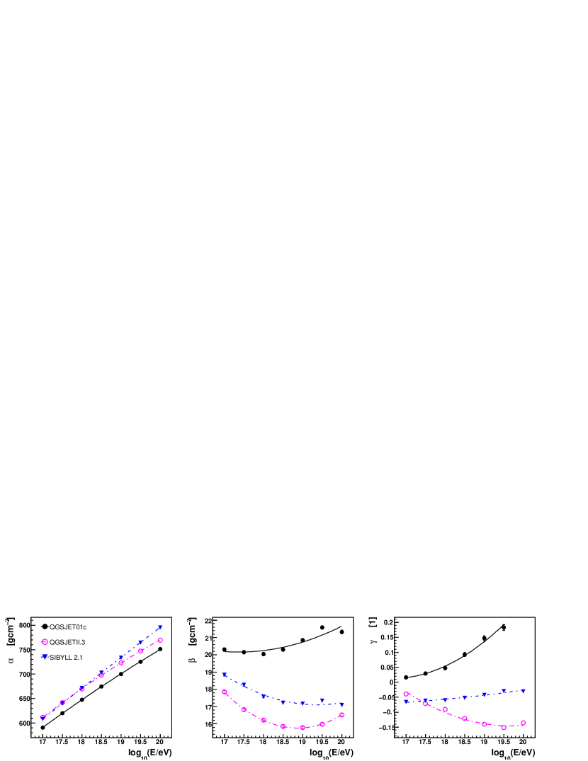
Figure 12: Parameterization of the energy dependence of the $\Delta X_{\rm 1}$-distributions. The lines denote the polynomial interpolations given in the text.

A.2 Cross section dependence

To infer the dependence of $P_{\Delta X_{1}}$ on $\lambda_{\rm p-air}$, a modified CONEX version [51] was used to generate $\Delta X_{1}$-distributions for several values of $f_{19}$, see Eq. (13). The energy dependence of all hadronic cross sections, i.e. p-, $\pi$-, and $K$-air interactions are then altered by the modification factor. This implies that the model uncertainties above $10^{15}\,\mathrm{eV}$ are rising proportional to the logarithm of the energy. This choice seems certainly reasonable, however, in the future also other energy dependences of $f(E)$ may turn out to be useful.

Table 3: Parameters for describing the cross section dependence of $\Delta X_{1}$-distributions.

Model	Index $i$	$\alpha^{\sigma}_{i}$ [g/cm]		$\beta^{\sigma}_{i}$ [g/cm]		$\gamma^{\sigma}_{i}$ [1]
QGSJet01c	$0$	730.09$\pm$	0.25	10.33$\pm$	0.00	0.03${\pm}$	0.03
	$1$	-33.61$\pm$	0.34	11.83$\pm$	0.00	0.10${\pm}$	0.03
	$2$	5.07$\pm$	0.09	-0.13$\pm$	0.00	0.20${\pm}$	0.07
	$3$					-0.01${\pm}$	0.01
QGSJetII.3	$0$	754.10$\pm$	0.27	8.46$\pm$	0.08	-0.25${\pm}$	0.02
	$1$	-35.86$\pm$	0.35	8.28$\pm$	0.19	0.10${\pm}$	0.02
	$2$	5.14$\pm$	0.09	-0.08$\pm$	0.01	-0.20${\pm}$	0.09
	$3$					0.02${\pm}$	0.00
SIBYLL 2.1	$0$	774.36$\pm$	0.27	11.67$\pm$	0.09	-0.18${\pm}$	0.04
	$1$	-46.36$\pm$	0.36	4.76$\pm$	0.16	0.10${\pm}$	0.04
	$2$	7.12$\pm$	0.10	0.12$\pm$	0.01	-0.00${\pm}$	0.15
	$3$					0.04${\pm}$	0.01

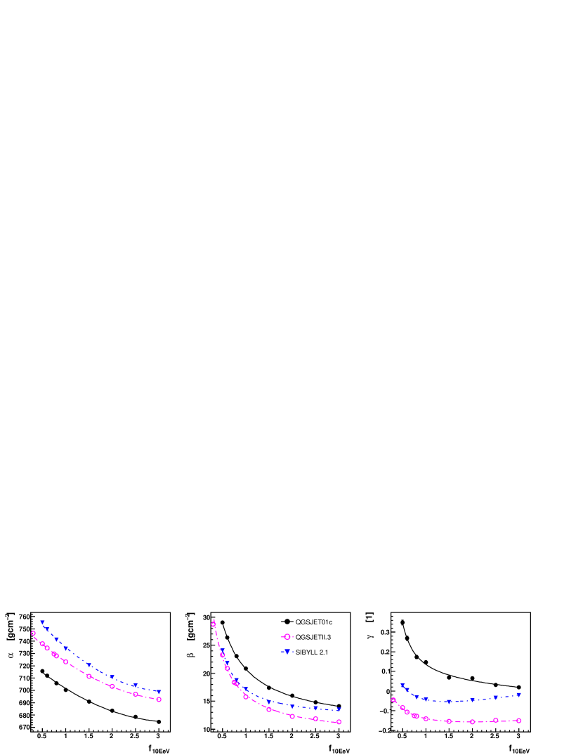
Figure 13: Parameterization of the $f_{19}$-dependence of the $\Delta X_{\rm 1}$-parameterizations with respect to a changing cross section. The lines denote the interpolations as discussed in the text.

The resulting dependence of $\Delta X_{\rm 1}$ on a changing cross section for air showers at $10^{19}\,\mathrm{eV}$ is shown in Fig. 13.

The dependence of the $\alpha$, $\beta$ and $\gamma$ parameters of the modified Moyal distribution on $f_{19}$ is parameterized as follows

$$\alpha^{\sigma}(f_{19}) =\alpha_{0}^{\sigma}+\alpha_{1}^{\sigma}\;f_{19}+\alpha_{2}^{\sigma}\;f_{19}^{2}$$

$$\beta^{\sigma}(f_{19}) =\beta_{0}^{\sigma}+\beta_{1}^{\sigma}/(f_{19}-\beta_{2}^{\sigma})$$ (17)

$$\gamma^{\sigma}(f_{19}) =\gamma_{0}^{\sigma}+\gamma_{1}^{\sigma}/(f_{19}-\gamma_{2}^{\sigma})+\gamma_{3}^{\sigma}\;f_{19}\;\;.$$

The resulting parameters of the interpolations are listed in Table 3. Furthermore, it is convenient to introduce the relative change as

$$\Delta\alpha^{\sigma}(f_{19}) =\alpha^{\sigma}(f_{19})-\alpha^{\sigma}(1)$$

$$\Delta\beta^{\sigma}(f_{19}) =\beta^{\sigma}(f_{19})-\beta^{\sigma}(1)$$ (18)

$$\Delta\gamma^{\sigma}(f_{19}) =\gamma^{\sigma}(f_{19})-\gamma^{\sigma}(1)\;\;.$$

A.3 Parameterization of the $\Delta X_{\rm 1}$-distribution

Combining the found dependence of $\Delta X_{\rm 1}$-distributions on the energy $E$ and the cross section modifier $f_{19}$, it is now possible to construct a parameterization of $P_{\Delta X_{1}}$ in terms of $E$ and $\sigma(E)$. Firstly, the principle energy dependence of $P_{\Delta X_{1}}$ is evaluated by calculating $\alpha^{\rm e}(E)$, $\beta^{\rm e}(E)$ and $\gamma^{\rm e}(E)$ using Eq. (A.1) and the results from Tab. 2. Secondly, the effect of the changed cross section is added. To achieve this, the first step is to calculate the corresponding deviation of the cross section $\sigma(E)$ extrapolated to $10^{19}\,\mathrm{eV}$ assuming Eq. (13). The resulting factor $f_{19}$ is then used to evaluate $\Delta\alpha^{\sigma}(f_{19})$, $\Delta\beta^{\sigma}(f_{19})$ and $\Delta\gamma^{\sigma}(f_{19})$ using Eq. (A.2) and the results listed in Tab. 3. In accordance to Eq. (13) the energy dependence is assumed to be logarithmic and vanishing below $10^{15}\,\mathrm{eV}$. This yields the final set of parameters of $P_{\Delta X_{1}}$

$$\alpha\bigl{(}E,\,\sigma(E)\bigr{)} =\alpha^{\rm e}\bigl{(}E\bigr{)}\;+\;F\bigl{(}E\bigr{)}\;\Delta\alpha^{\sigma}\bigl{(}f_{19}\bigr{)}$$

$$\beta\bigl{(}E,\,\sigma(E)\bigr{)} =\beta^{\rm e}\bigl{(}E\bigr{)}\;+\;F\bigl{(}E\bigr{)}\;\Delta\beta^{\sigma}\bigl{(}f_{19}\bigr{)}$$ (19)

$$\gamma\bigl{(}E,\,\sigma(E)\bigr{)} =\gamma^{\rm e}\bigl{(}E\bigr{)}\;+\;F\bigl{(}E\bigr{)}\;\Delta\gamma^{\sigma}\bigl{(}f_{19}\bigr{)}\,,$$

with

$$F(E)=\left\{\begin{array}[]{l l}0&\quad E\leq 10^{15}\,\mathrm{eV}\\ \ln(E/1\,\mbox{PeV})/\ln(10\,\mbox{EeV}/1\,\mbox{PeV})&\quad E>10^{15}\,\mathrm{eV}\end{array}\right.\,.$$ (20)

Bibliography

Bibliography

- [1] B. Bodhaine et al., J. Atmos. Ocean. Tech. 16 (1999) 1854.
- [2] N. Grigorov et al., Proc. of 9th Int. Cosmic Ray Conf, London 1 (1965) 860.
- [3] G. Yodh, Y. Pal, and J. Trefil, Phys. Rev. Lett. 28 (1972) 1005–1008.
- [4] R. Nam, S. Nikolsky, V. Pavluchenko, A. Chubenko, and V. Yakovlev, Proc. of 14th Int. Cosmic Ray Conf, Munich (1975) 2258.
- [5] F. Siohan et al., J. Phys. G4 (1978) 1169–1186.
- [6] H. Mielke, M. Foeller, J. Engler, and J. Knapp, J. Phys. G20 (1994) 637–649.
- [7] T. Hara et al., Phys. Rev. Lett. 50 (1983) 2058–2061.
- [8] M. Honda et al., Phys. Rev. Lett. 70 (1993) 525–528.
- [9] N. Nikolaev, Phys. Rev. D48 (1993) 1904–1906 and hep-ph/9304283.
- [10] M. Aglietta et al., Phys. Rev. D79 (2009) 032004.
- [11] R. Baltrusaitis et al., Phys. Rev. Lett. 52 (1984) 1380–1383.
- [12] S. Knurenko, V. Sleptsova, I. Sleptsov, N. Kalmykov, and S. Ostapchenko, Proc. of 26th Int. Cosmic Ray Conf., Salt Lake City, Utah 1 (1999) 372.
- [13] K. Belov, Nucl. Phys. (Proc. Suppl.) 151 (2006) 197–204.
- [14] G. Aielli et al., submitted to Phys. Rev. D (2009) and arXiv:0904.4198 [hep-ex].
- [15] T. K. Gaisser et al. (HIRES Collab.), Phys. Rev. D47 (1993) 1919–1932.
- [16] N. Kalmykov, S. Ostapchenko, and A. Pavlov, Nucl. Phys. (Proc. Suppl.) B52 (1997) 17–28.
- [17] S. Ostapchenko, Phys. Rev. D74 (2006) 014026 and hep-ph/0505259.
- [18] R. Engel, T. Gaisser, T. Stanev, and P. Lipari, Proc. of 26th Int. Cosmic Ray Conf., Salt Lake City, Utah 1 (1999) 415.
- [19] R. Fletcher, T. Gaisser, P. Lipari, and T. Stanev, Phys. Rev. D50 (1994) 5710–5731.
- [20] K. Werner and T. Pierog, AIP Conf. Proc. 928 (2007) 111–117 and arXiv:0707.3330 [astro-ph].
- [21] S. Ostapchenko, Nucl. Phys. Proc. Suppl. 151 (2006) 143–146 and hep-ph/0412332.
- [22] R. Engel, T. Gaisser, P. Lipari, and T. Stanev, Phys. Rev. D58 (1998) 014019 and hep-ph/9802384.
- [23] V. Berezinsky, A. Gazizov, and S. Grigorieva, Phys. Lett. B612 (2005) 147–153 and astro-ph/0502550.
- [24] V. Berezinsky, S. Grigoreva, and B. Hnatyk, Nucl. Phys. (Proc. Suppl.) 151 (2006) 497–500.
- [25] V. Berezinsky, Proc. of 30th Int. Cosmic Ray Conf., Merida, Mexico (2007) and arXiv:0710.2750 [astro-ph].
- [26] G. Zatsepin and V. Kuzmin, JETP Lett. 4 (1966) 78–80.
- [27] K. Greisen, Phys. Rev. Lett. 16 (1966) 748–750.
- [28] J. Abraham et al. (Pierre Auger Collab.), Science 318 (2007) 938–943 and arXiv:0711.2256 [astro-ph].
- [29] R. Abbasi et al. (HiRes Collab.), Phys. Rev. Lett. 100 (2008) 101101 and astro-ph/0703099.
- [30] J. Abraham et al. (Pierre Auger Collab.), Phys. Rev. Lett. 101 (2008) 061101 and arXiv:0806.4302 [astro-ph].
- [31] R. Ulrich et al., in preparation (2009) .
- [32] R. Abbasi et al. (HiRes Collab.), Astrophys. J. 622 (2005) 910–926 and astro-ph/0407622.
- [33] J. Abraham et al. (Pierre Auger Collab.), Nucl. Instrum. Meth. A523 (2004) 50.
- [34] H. Kawai et al. (TA Collab.), Nucl. Phys. Proc. Suppl. 175-176 (2008) 221–226.
- [35] L. Landau and I. Pomeranchuk, Dokl. Akad. Nauk Ser. Fiz. 92 (1953) 535–536.
- [36] L. Landau and I. Pomeranchuk, Dokl. Akad. Nauk Ser. Fiz. 92 (1953) 735–738.
- [37] A. Migdal, Phys. Rev. 103 (1956) 1811–1820.
- [38] T. Bergmann et al., Astropart. Phys. 26 (2007) 420–432 and astro-ph/0606564.
- [39] J. Alvarez-Muniz, R. Engel, T. Gaisser, J. Ortiz, and T. Stanev, Phys. Rev. D66 (2002) 123004 and astro-ph/0209117.
- [40] B. Rossi and K. Greisen, Rev. Mod. Phys. 13 (1941) 240–309.
- [41] P. Billoir, http://www-ik.fzk.de/corsika/corsika-school2008/talks/ CORSIKA School, 2008.
- [42] F. Nerling, J. Blümer, R. Engel, and M. Risse, Astropart. Phys. 24 (2006) 421–437.
- [43] M. Giller, A. Kacperczyk, J. Malinowski, W. Tkaczyk, and G. Wieczorek, J. Phys. G31 (2005) 947–958.
- [44] S. Lafebre et al., Astropart. Phys. 31 (2009) 243–254 and arXiv:0902.0548 [astro-ph.HE].
- [45] P. Lipari, Phys. Rev. 79 (2008) 063001 and arXiv:0809.0190 [astro-ph].
- [46] R. Ellsworth, T. Gaisser, T. Stanev, and G. Yodh, Phys. Rev. D26 (1982) 336.
- [47] R. Baltrusaitis et al. (Fly’s Eye Collab.), Nucl. Instrum. Meth. A240 (1985) 410.
- [48] H. Barbosa, F. Catalani, J. A. Chinellato, and C. Dobrigkeit, Astropart. Phys. 22 (2004) 159–166 and astro-ph/0310234.
- [49] B. R. Dawson (Pierre Auger Collab.), Proc. of 30th Int. Cosmic Ray Conf., Merida, Mexico (2007) and arXiv:0706.1105 [astro-ph].
- [50] R. Ulrich, J. Blümer, R. Engel, F. Schüssler, and M. Unger, Proc. of XIV ISVHECRI, Weihai, China (2006) and astro-ph/0612205.
- [51] R. Ulrich et al., in preparation (2009) .
- [52] J. Abraham et al. (Pierre Auger Collab.), Astropart. Phys. 29 (2008) 243–256 and arXiv:0712.1147 [astro-ph].
- [53] J. Alvarez-Muniz, R. Engel, T. Gaisser, J. Ortiz, and T. Stanev, Phys. Rev. D69 (2004) 103003 and astro-ph/0402092.
- [54] M. Block, Phys. Rev. D76 (2007) 111503 and arXiv:0705.3037 [hep-ph].