Percolation Thresholds of the Fortuin-Kasteleyn Cluster for the Edwards-Anderson Ising Model on Complex Networks

Abstract

We analytically show the percolation thresholds of the Fortuin-Kasteleyn cluster for the Edwards-Anderson Ising model on random graphs with arbitrary degree distributions. The results on the Nishimori line are shown. We obtain the results for the $\pm J$ model, the diluted $\pm J$ model, and the Gaussian model, by applying an extension of a criterion for the random graphs with arbitrary degree distributions. The results for the infinite-range $\pm J$ model and the Sherrington-Kirkpatrick model are also shown.

1 Introduction

The study of complex networks has been carried out, and the study of spin models on the complex networks is important [1]. As an example of such a spin model, we study in this article spin models on random graphs with arbitrary degree distributions. The behavior of spins on a no growing network is investigated.

We investigate the Edwards-Anderson Ising model [2] as an Ising spin-glass model. The understanding of the Edwards-Anderson Ising model on random graphs and on the Bethe lattice is still incomplete [1, 3, 4]. In this article, the $\pm J$ model, the diluted $\pm J$ model, and the Gaussian model for the Edwards-Anderson Ising model are investigated. For those models, there is a special line, called the Nishimori line, on the phase diagram for the exchange interactions and the temperature. The internal energy, the upper bound of the specific heat, and so forth are exactly calculated on the Nishimori line [5, 6, 7, 8, 9]. The location of the multicritical point for the Edwards-Anderson Ising model on the square lattice is conjectured, and it is shown that the conjectured value is in good agreement with other numerical estimates [10]. In this article, the results on the Nishimori line are shown.

There is a case where a percolation transition of networks occures. A network is divided into many networks by deleting some of its nodes and/or links. We call this percolation transition ‘the percolation transition of network’ in this article. There is also a case where a percolation transition of clusters occurs. A cluster consists of fictitious bonds. The bond is put between spins. One of the clusters becomes a giant component when a cluster is percolated. We call this percolation transition ‘the percolation transition of clusters’, and discuss the percolation transition of a cluster on a complex network.

In this article, the percolation transition of the Fortuin-Kasteleyn (FK) cluster is investigated. The FK cluster has the FK representation [11, 12]. In the ferromagnetic Ising model, the percolation transition point agrees with the phase transition point. The agreement is described in Ref. CK. Powerful Monte Carlo methods using the FK cluster have been proposed [14, 15, 16, 17, 18]. The Edwards-Anderson Ising model has a conflict in the interactions: the percolation transition point disagrees with the phase transition point. There are numerous approches for resolving the disagreement by extending the FK representation [19]. On the other hand, it was pointed out by de Arcangelis et al. that the correct understanding of the percolation phenomenon of the FK cluster in the Edwards-Anderson Ising model is important since a dynamical transition occurs at a temperature very close to the percolation temperature, and the dynamical transition and percolation transition are related to a transition for a signal propagating between spins [20]. The dynamical transition is characterized by a parameter called the Hamming distance or damage [20]. In this article, the percolation threshold is analytically found.

The study of random graphs with arbitrary degree distributions has been carried out [21]. Our results are obtained by applying an extension of a criterion [22, 23, 24] for random graphs with arbitrary degree distributions. The results for the infinite-range $\pm J$ model and the Sherrington-Kirkpatrick (SK) model [25] are also shown.

This article is organized as follows. First in §2, a complex network model and the Edwards-Anderson Ising model are described. Next in §3, the FK cluster is explained. After elucidating a criterion for the percolation of a cluster in §4, we will in §5 find the percolation thresholds for the $\pm J$ model and the diluted $\pm J$ model. The result for the Gaussian model is shown in §6. The final section is devoted to a summary.

2 A complex network model and the Edwards-Anderson Ising model

A network consists of nodes and links. A link connects nodes. In this article, as a complex network model, random graphs with arbitrary degree distributions are investigated. The network has no correlation between nodes. The node degree, $k$, is given with a distribution $p(k)$. The links are randomly connected between nodes.

We define a variable $b(i,j)$, where $b(i,j)$ is one when nodes $i$ and $j$ are connected by a link. $b(i,j)$ is zero when nodes $i$ and $j$ are not connected by a link. The degree $k(i)$ of node $i$ is given by

$$k(i)=\sum_{j}b(i,j)\,.$$ (1)

The coordination number (the average of the node degree for links), $\langle k\rangle_{N}$, is given by

$$\langle k\rangle_{N}=\frac{1}{N}\sum_{i}^{N}k(i)\,,$$ (2)

where $\langle\,\rangle_{N}$ is the average over the entire network. $N$ is the number of nodes. The average of the square of the node degree for links, $\langle k^{2}\rangle_{N}$, is given by

$$\langle k^{2}\rangle_{N}=\frac{1}{N}\sum_{i}^{N}k^{2}(i)\,.$$ (3)

We define

$$a=\frac{2\langle k\rangle_{N}}{\langle k^{2}\rangle_{N}}\,,$$ (4)

where $a$ represents an aspect of the network.

Figure 1: Relation between the aspect $a$ and the model on the network.

Figure 1 shows the relation between the aspect $a$ and the model on the network. The network is almost a complete graph when $a$ is close to zero, and the model on the network is almost an infinite-range model. The model on the network is the infinite-range model when $\langle k\rangle_{N}=N-1$, $\langle k^{2}\rangle_{N}=(N-1)^{2}$, and $a=2/(N-1)$. The network consists of many cycle graphs when the coordination number $\langle k\rangle_{N}$ is two. The model on the network consists of many chain models when $\langle k\rangle_{N}$ is two. In the Erdős-Rényi (ER) random graph model and in the Gilbert model, the distribution of node degree is the Poisson distribution [1]. The ER random graph model is a network model wherein the network consists of a fixed number of nodes and a fixed number of links, and the links are randomly connected between the nodes. The Gilbert model is a network model wherein the link between nodes is connected with a given probability. In the ER random graph model and in the Gilbert model, $\langle k\rangle_{N}=1$ and $\langle k^{2}\rangle_{N}=\langle k\rangle_{N}(\langle k\rangle_{N}+1)=2$ when $a$ is one.

The Hamiltonian for the Edwards-Anderson Ising model, ${\cal H}$, is given by

$${\cal H}=-\sum_{\langle i,j\rangle}J_{i,j}S_{i}S_{j}\,,$$ (5)

where $\langle i,j\rangle$ denotes nearest-neighbor pairs, $S_{i}$ denotes the state of the spin at node $i$, and $S_{i}=\pm 1$. $J_{i,j}$ is the strength of the exchange interaction between spins. The value of $J_{i,j}$ is given by the distribution $P(J_{i,j})$. The $\pm J$ model, the diluted $\pm J$ model, and the Gaussian model are given by specific $P(J_{i,j})$.

For the $\pm J$ model, the distribution $P^{(\pm J)}(J_{ij})$ is given by

$$P^{(\pm J)}(J_{i,j})=p\,\delta_{J_{i,j},J}+(1-p)\,\delta_{J_{i,j},-J}\,,$$ (6)

where $J>0$. $p$ is the probability that the interaction is ferromagnetic ($J_{i,j}=J$). $1-p$ is the probability that the interaction is antiferromagnetic ($J_{i,j}=-J$).

For the diluted $\pm J$ model, the distribution $P^{({\rm D}\pm J)}(J_{i,j})$ is given by

$$P^{({\rm D}\pm J)}(J_{i,j})=p\,\delta_{J_{i,j},J}+q\,\delta_{J_{i,j},-J}+r\,\delta_{J_{i,j},0}\,,$$ (7)

where $J>0$ and $p+q+r=1$. $p$ is the probability that the interaction is ferromagnetic ($J_{i,j}=J$). $q$ is the probability that the interaction is antiferromagnetic ($J_{i,j}=-J$). $r$ is the probability that the interaction is diluted ($J_{i,j}=0$). This model is the $\pm J$ model when $r=0$.

For the Gaussian model, the distribution $P^{({\rm Gaussian})}(J_{i,j})$ is given by

$$P^{(\rm Gaussian)}(J_{i,j})=\frac{1}{\sqrt{2\pi J^{2}}}e^{-(J_{i,j}-J_{0})^{2}/2J^{2}}\,.$$ (8)

The average of $J_{i,j}$ is given by $[J_{i,j}]_{R}=J_{0}$, where $[\,]_{R}$ is the random configuration average. The variance of $J_{i,j}$ is given by $[J^{2}_{i,j}]_{R}-[J_{i,j}]^{2}_{R}=J^{2}$.

To calculate thermodynamic quantities, a gauge transformation [5, 6, 7, 8, 9, 26] wherein the transformation is performed by

$$J_{i,j}\to J_{i,j}\sigma_{i}\sigma_{j}\,,\quad S_{i}\to S_{i}\sigma_{i}$$ (9)

is used, where $\sigma_{i}=\pm 1$. It is known that the gauge transformation has no effect on thermodynamic quantities [26]. Following the gauge transformation, the ${\cal H}$ part becomes ${\cal H}\to{\cal H}$ and the $P(J_{i,j})$ part becomes $P(J_{i,j})\to P(J_{i,j}\sigma_{i}\sigma_{j})$.

3 The Fortuin-Kasteleyn cluster

The bond for the FK cluster is put between spins with probability $P_{\rm FK}(S_{i},S_{j},J_{ij})$. The value of $P_{\rm FK}$ depends on the interaction between spins and the states of spins. We call the bond the FK bond in this article. $P_{\rm FK}(S_{i},S_{j},J_{ij})$ is given by [20]

$$P_{\rm FK}(S_{i},S_{j},J_{ij})=1-e^{-\beta J_{ij}S_{i}S_{j}-\beta|J_{ij}|}\,,$$ (10)

where $\beta$ is the inverse temperature and $\beta=1/k_{B}T$. $k_{B}$ is the Boltzmann constant and $T$ is the temperature. By connecting the FK bonds, the FK clusters are generated. By the gauge transformation, the $P_{\rm FK}$ part becomes $P_{\rm FK}\to P_{\rm FK}$.

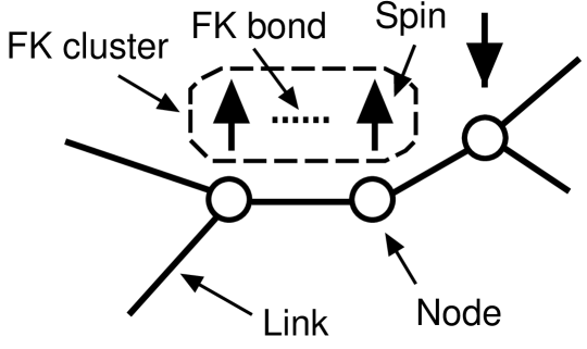
Figure 2: Network and FK cluster. Three nodes, six links, three spins, an FK bond, and an FK cluster are depicted. Spins are aligned on each node. The percolation of the FK cluster is discussed in this article.

Figure 2 shows a conceptual diagram of a network and an FK cluster. Three nodes, six links, three spins, an FK bond, and an FK cluster are depicted. Spins are aligned on each node. The percolation of the FK cluster is discussed in this article.

The thermodynamic quantity of the FK bond put between the spins on nodes $i$ and $j$, $[\langle b_{\rm FK}(i,j)\rangle_{T}]_{R}$, is given by

$$[\langle b_{\rm FK}(i,j)\rangle_{T}]_{R}=[\langle P_{\rm FK}(S_{i},S_{j},J_{i,j})\rangle_{T}]_{R}\,,$$ (11)

where $\langle\,\rangle_{T}$ is the thermal average. The thermodynamic quantity of the node degree for FK bonds at node $i$, $[\langle k_{\rm FK}(i)\rangle_{T}]_{R}$, is given by

$$[\langle k_{\rm FK}(i)\rangle_{T}]_{R}=$$

$$\quad[\langle\sum_{\{j|b(i,j)=1\}}P_{\rm FK}(S_{i},S_{j},J_{i,j})\rangle_{T}]_{R}\,.$$ (12)

The thermodynamic quantity of the square of the node degree for FK bonds at node $i$, $[\langle k^{2}_{\rm FK}(i)\rangle_{T}]_{R}$, is given by

$$[\langle k^{2}_{\rm FK}(i)\rangle_{T}]_{R}=$$ (13)

$$[\langle\sum_{\{j|b(i,j)=1\}}\sum_{\{l|b(i,l)=1\}}P_{\rm FK}(S_{i},S_{j},J_{i,j})$$

$$\times P_{\rm FK}(S_{i},S_{l},J_{i,l})(1-\delta_{j,l})$$

$$+ \sum_{\{j|b(i,j)=1\}}P_{\rm FK}(S_{i},S_{j},J_{i,j})\rangle_{T}]_{R}\,.$$

The thermodynamic quantity of the node degree for FK bonds, $[\langle k_{\rm FK}\rangle_{T}]_{R}$, is given by

$$[\langle k_{\rm FK}\rangle_{T}]_{R}=\frac{1}{N}\sum_{i}^{N}[\langle k_{\rm FK}(i)\rangle_{T}]_{R}\,.$$ (14)

The thermodynamic quantity of the square of the node degree for FK bonds, $[\langle k^{2}_{\rm FK}\rangle_{T}]_{R}$, is given by

$$[\langle k^{2}_{\rm FK}\rangle_{T}]_{R}=\frac{1}{N}\sum_{i}^{N}[\langle k^{2}_{\rm FK}(i)\rangle_{T}]_{R}\,.$$ (15)

4 A criterion for percolation of clusters

The percolation of the random graphs with arbitrary degree distributions occurs when [22, 23, 24]

$$\langle k^{2}\rangle_{N}\,\geq\,2\langle k\rangle_{N}\,.$$ (16)

Equation (16) is the inequality when the network is percolated. Equation (16) is the equality when the network is at the percolation transition point. The criterion (Eq. (16)) is true for a sufficiently large number of nodes. Equation (16) is derived by Molly and Reed [22], Cohen et al. [23], and Newman et al. [24].

From Eq. (16), the network is percolated when $a<1$ and the network is at the percolation transition point when $a=1$. The network is unpercolated when $a>1$. Therefore, the percolation of clusters is investigated for $0<a\leq 1$.

When links and/or nodes are randomly diluted on the random graphs with arbitrary degree distributions, the criterion (Eq. (16)) is applicable to the diluted network [23]. The percolation problem for the diluted network can be regarded as the random-bond percolation problem. We define the bond states as the graph $G$. We define the node degree for random bonds at node $i$ as $k_{\rm random\,bond}(G,i)$. The random bonds are randomly put on the links, and the links are randomly connected between the nodes. The criterion of the percolation of clusters for the random-bond percolation problem is given by

$$\frac{1}{N}\sum_{i}k_{\rm random\,bond}^{2}(G,i)\geq\frac{2}{N}\sum_{i}k_{\rm random\,bond}(G,i)\,.$$ (17)

In what follows, a criterion of the percolation of clusters for spin models is conjectured on the basis of the above discussion.

We consider a case that the magnitude of a bond does not depend on the degree $k(i)$. The bond is a bond put between spins and includes the FK bond. We define a variable for the inverse temperature as $\rho(\beta)$. We set

$$0<\rho(\beta)\leq 1\,.$$ (18)

We consider a case that $[\langle b_{\rm bond}(i,j)\rangle_{T}]_{R}$, $[\langle k_{\rm bond}(i)\rangle_{T}]_{R}$, and $[\langle k^{2}_{\rm bond}(i)\rangle_{T}]_{R}$ are respectively written as

$$[\langle b_{\rm bond}(i,j)\rangle_{T}]_{R}=\rho(\beta)\,,$$ (19)

$$[\langle k_{\rm bond}(i)\rangle_{T}]_{R}=\rho(\beta)\,k(i)\,,$$ (20)

$$[\langle k^{2}_{\rm bond}(i)\rangle_{T}]_{R} = \rho^{2}(\beta)\,k(i)[k(i)-1]$$ (21)

$$+ \rho(\beta)\,k(i)\,.$$

In this case, it is implied that the bias for $k(i)$ does not appear in the statistical results of the bonds. Therefore, we describe the case that $[\langle b_{\rm bond}(i,j)\rangle_{T}]_{R}$, $[\langle k_{\rm bond}(i)\rangle_{T}]_{R}$, and $[\langle k^{2}_{\rm bond}(i)\rangle_{T}]_{R}$ are respectively written as Eqs. (19), (20), and (21) as the case that the magnitude of the bond does not depend on $k(i)$.

When the magnitude of the bond does not depend on $k(i)$, as an extension of Eq. (17), we conjecture

$$\frac{1}{N}\sum_{i}k_{\rm bond}^{2}(\{S_{j}\},\{J_{j,l}\},G,i)\geq$$

$$\quad\frac{2}{N}\sum_{i}k_{\rm bond}(\{S_{j}\},\{J_{j,l}\},G,i)\,.$$ (22)

Since the magnitude of the bond does not depend on $k(i)$, the bonds are randomly put on links, and the links are randomly connected between nodes. $\{S_{j}\}$ is a subset of spin states. $\{J_{j,l}\}$ is a subset of exchange interactions. $k_{\rm bond}(\{S_{j}\},\{J_{j,l}\},G,i)$ is the node degree for bonds at node $i$ in the graph $G$ that is compatible with $\{S_{j}\}$ and $\{J_{j,l}\}$. Equation (17) is true for a sufficiently large number of nodes. Therefore, Eq. (22) may also be true for a sufficiently large number of nodes when the magnitude of the bond does not depend on $k(i)$. By using Eq. (22), we obtain a conjectured criterion of the percolation of clusters for spin models as

$$[\langle k^{2}_{\rm bond}\rangle_{T}]_{R}\geq 2[\langle k_{\rm bond}\rangle_{T}]_{R}\,.$$ (23)

Equation (23) is the inequality when the cluster is percolated. Equation (23) is the equality when the cluster is at the percolation transition point. Equation (23) gives the percolation threshold of the clusters.

5 The $\pm J$ model and the diluted $\pm J$ model

By using Eq. (6), the distribution $P^{(\pm J)}(J_{i,j})$ is written as

$$P^{(\pm J)}(J_{i,j})=\frac{e^{\beta_{P}J_{i,j}}}{2\cosh(\beta_{P}J)}\,,\quad J_{i,j}=\pm J\,,$$ (24)

where $\beta_{P}$ is given by [5, 6, 7, 8]

$$\beta_{P}=\frac{1}{2J}\ln\frac{p}{1-p}\,.$$ (25)

When the value of $\beta_{P}$ is consistent with the value of the inverse temperature $\beta$, the line on the phase diagram obtained using Eq. (25) is called the Nishimori line. By using the gauge transformation, the distribution $P^{(\pm J)}(J_{i,j})$ part becomes

$$\prod_{\langle i,j\rangle}P^{(\pm J)}(J_{i,j}) = \frac{e^{\beta_{P}\sum_{\langle i,j\rangle}J_{i,j}}}{[2\cosh(\beta_{P}J)]^{N_{B}}}$$ (26)

$$\to \frac{\sum_{\{\sigma_{i}\}}e^{\beta_{P}\sum_{\langle i,j\rangle}J_{i,j}\sigma_{i}\sigma_{j}}}{2^{N}[2\cosh(\beta_{P}J)]^{N_{B}}}\,,$$

where $N_{B}$ is the number of nearest-neighbor pairs in the whole system.

By using Eqs. (9), (10), (11), and (26), when $\beta=\beta_{P}$, the thermodynamic quantity of the FK bond put between the spins on nodes $i$ and $j$, $[\langle b_{\rm FK}(i,j)\rangle_{T}]^{(\pm J)}_{R}$, is obtained as

$$[\langle b_{\rm FK}(i,j)\rangle_{T}]^{(\pm J)}_{R}$$ (27)

$$= \sum_{\{J_{l,m}\}}\prod_{\langle l,m\rangle}P^{(\pm J)}(J_{l,m})$$

$$\times \frac{\sum_{\{S_{l}\}}P_{\rm FK}(S_{i},S_{j},J_{i,j})\,e^{\beta_{P}\sum_{\langle l,m\rangle}J_{l,m}S_{l}S_{m}}}{\sum_{\{S_{l}\}}e^{\beta_{P}\sum_{\langle l,m\rangle}J_{l,m}S_{l}S_{m}}}$$

$$= \frac{1}{2^{N}[2\cosh(\beta_{P}J)]^{N_{B}}}$$

$$\times \sum_{\{J_{l,m}\}}\sum_{\{S_{l}\}}P_{\rm FK}(S_{i},S_{j},J_{i,j})\,e^{\beta_{P}\sum_{\langle l,m\rangle}J_{l,m}S_{l}S_{m}}$$

$$= \tanh(\beta_{P}J)\,.$$

By using Eqs. (9), (10), (12), and (26), when $\beta=\beta_{P}$, the thermodynamic quantity of the node degree for FK bonds at node $i$, $[\langle k_{\rm FK}(i)\rangle_{T}]^{(\pm J)}_{R}$, is obtained as

$$[\langle k_{\rm FK}(i)\rangle_{T}]^{(\pm J)}_{R}=\tanh(\beta_{P}J)\,k(i)\,.$$ (28)

By using Eqs. (9), (10), (13), and (26), when $\beta=\beta_{P}$, the thermodynamic quantity of the square of the node degree for FK bonds at node $i$, $[\langle k^{2}_{\rm FK}(i)\rangle_{T}]^{(\pm J)}_{R}$, is obtained as

$$[\langle k^{2}_{\rm FK}(i)\rangle_{T}]^{(\pm J)}_{R} = \tanh^{2}(\beta_{P}J)\,k(i)[k(i)-1]$$ (29)

$$+ \tanh(\beta_{P}J)\,k(i)\,.$$

We set

$$\rho^{(\pm J)}(\beta_{P})=\tanh(\beta_{P}J)\,.$$ (30)

Equations (27), (28), (29), and (30) are formulated as Eqs. (19), (20), and (21). Therefore, the magnitude of the FK bond does not depend on $k(i)$. By using Eqs. (14), (15), (23), (28), and (29), we obtain

$$1-\exp(-2\beta_{P}J)\geq\frac{2\langle k\rangle_{N}}{\langle k^{2}\rangle_{N}}\,.$$ (31)

Equation (31) is the inequality when the FK cluster is percolated. Equation (31) is the equality when the FK cluster is at the percolation transition point.

From Eqs. (18) and (30), there is the percolation transition point for $0<\beta_{P}\leq\infty$. From Eq. (31), there is the percolation transition point for $0<a\leq 1$. By using Eqs. (25) and (31), the probability $p^{(\pm J)}$ that the interaction is ferromagnetic is obtained as

$$p^{(\pm J)}=\frac{1}{2-a}$$ (32)

at the percolation transition point. By using Eqs. (25) and (32), the percolation transition temperature $T^{(\pm J)}_{P}$ is obtained as

$$T^{(\pm J)}_{P}=\frac{J}{k_{B}}\frac{2}{\ln\frac{1}{1-a}}\,.$$ (33)

Figure 3: Percolation threshold of the FK cluster for the $\pm J$ model. (a) The relation between the aspect $a$ and the probability $p^{(\pm J)}$ is shown. (b) The relation between the aspect $a$ and the percolation transition temperature $T^{(\pm J)}_{P}$ is shown. $J/k_{B}$ is set to $1$.

Figure 3 shows the percolation threshold of the FK cluster for the $\pm J$ model. Figure 3(a) shows the relation between the aspect $a$ and the probability $p^{(\pm J)}$. Equation (32) is used for showing Fig. 3(a). Figure 3(b) shows the relation between the aspect $a$ and the percolation transition temperature $T^{(\pm J)}_{P}$. Equation (33) is used for showing Fig. 3(b). $J/k_{B}$ is set to $1$.

For the ferromagnetic Ising model on the same network, the phase transition temperature $T^{({\rm Ferro})}_{C}$ is [27, 28]

$$T^{({\rm Ferro})}_{C}=\frac{J}{k_{B}}\frac{2}{\ln\frac{1}{1-a}}\,.$$ (34)

$T^{(\pm J)}_{P}$ (Eq. (33)) coincides with $T^{({\rm Ferro})}_{C}$.

The complete graph is considered as $a\sim 0$. We set $\langle k\rangle_{N}=N-1$, $\langle k^{2}\rangle_{N}=(N-1)^{2}$, $a=2/(N-1)$, and $J\to J/\sqrt{N}$. From the settings, the model on the network becomes the infinite-range $\pm J$ model. By using Eq. (32), the probability $p^{({\rm IR}\pm J)}$ that the interaction is ferromagnetic is obtained as

$$p^{({\rm IR}\pm J)}=\frac{N-1}{2(N-2)}\to\frac{1}{2}$$ (35)

for a sufficiently large number of nodes at the percolation transition point. By using Eq. (33), the percolation transition temperature $T^{({\rm IR}\pm J)}_{P}$ is obtained as

$$T^{({\rm IR}\pm J)}_{P}=\frac{J}{k_{B}\sqrt{N}}\frac{2}{\ln(1+\frac{2}{N-3})}\to\frac{J}{k_{B}}\sqrt{N}$$ (36)

for a sufficiently large number of nodes.

In Ref. MNS, the percolation transition temperature of the FK cluster for the infinite-range $\pm J$ model is derived by using the analytical solution of the SK model. The percolation transition temperature of the FK cluster for the infinite-range $\pm J$ model obtained in this article agrees with the result for a single-replica case in Ref. MNS. Therefore, we were able to confirm that our result is exact at this extremal point.

We consider the case for $a=1$. By using Eq. (32), we obtain $p=1$. By using Eq. (33), we obtain $T_{P}=0$. From Eq. (16), the network is at the percolation transition point. From $p=1$, the exchange interaction is only the ferromagnetic interaction. From $T_{P}=0$, all the spins are parallel. From $p=1$ and $T_{P}=0$, we obtain $P_{\rm FK}=1$ for all nearest-neighbor pairs. Therefore, the FK cluster and the network are at the percolation transition point. We were able to confirm that our result is exact at this extremal point.

By using Eq. (7), the distribution $P^{({\rm D}\pm J)}(J_{ij})$ for the diluted $\pm J$ model is written as

$$P^{({\rm D}\pm J)}(J_{i,j})=\frac{e^{\beta^{(2)}_{P}J^{2}_{i,j}+\beta_{P}J_{ij}}}{e^{\beta^{(2)}_{P}J^{2}+\beta_{P}J}+1+e^{\beta^{(2)}_{P}J^{2}-\beta_{P}J}}\,,$$ (37)

where $\beta_{P}^{(2)}$ and $\beta_{P}$ are respectively [9]

$$\beta^{(2)}_{P}=\frac{1}{J^{2}}\ln\sqrt{\frac{pq}{r^{2}}}\,,\quad\beta_{P}=\frac{1}{J}\ln\sqrt{\frac{p}{q}}\,.$$ (38)

This model becomes the $\pm J$ model when $r=0$. In what follows, the result for $r\neq 0$ is only described since the result for the $\pm J$ model is described above. By using the gauge transformation, the distribution $P^{({\rm D}\pm J)}(J_{i,j})$ part becomes

$$\prod_{\langle i,j\rangle}P^{({\rm D}\pm J)}(J_{i,j})$$ (39)

$$= \frac{e^{\beta^{(2)}_{P}\sum_{\langle i,j\rangle}J^{2}_{i,j}+\beta_{P}\sum_{\langle i,j\rangle}J_{i,j}}}{(e^{\beta^{(2)}_{P}J^{2}+\beta_{P}J}+1+e^{\beta^{(2)}_{P}J^{2}-\beta_{P}J})^{N_{B}}}$$

$$\to \frac{\sum_{\{\sigma_{i}\}}e^{\beta^{(2)}_{P}\sum_{\langle i,j\rangle}J^{2}_{i,j}+\beta_{P}\sum_{\langle i,j\rangle}J_{i,j}\sigma_{i}\sigma_{j}}}{2^{N}(e^{\beta^{(2)}_{P}J^{2}+\beta_{P}J}+1+e^{\beta^{(2)}_{P}J^{2}-\beta_{P}J})^{N_{B}}}\,.$$

By using Eqs. (9), (10), (11), and (39), when $\beta=\beta_{P}$, the thermodynamic quantity of the FK bond put between the spins on nodes $i$ and $j$, $[\langle b_{\rm FK}(i,j)\rangle_{T}]^{({\rm D}\pm J)}_{R}$, is obtained as

$$[\langle b_{\rm FK}(i,j)\rangle_{T}]^{({\rm D}\pm J)}_{R}$$ (40)

$$= \sum_{\{J_{l,m}\}}\prod_{\langle l,m\rangle}P^{({\rm D}\pm J)}(J_{l,m})$$

$$\times \frac{\sum_{\{S_{l}\}}P_{\rm FK}(S_{i},S_{j},J_{i,j})\,e^{\beta_{P}\sum_{\langle l,m\rangle}J_{l,m}S_{l}S_{m}}}{\sum_{\{S_{l}\}}e^{\beta_{P}\sum_{\langle l,m\rangle}J_{l,m}S_{l}S_{m}}}$$

$$= \frac{1}{2^{N}(e^{\beta^{(2)}_{P}J^{2}+\beta_{P}J}+1+e^{\beta^{(2)}_{P}J^{2}-\beta_{P}J})^{N_{B}}}$$

$$\times \sum_{\{J_{l,m}\}}\sum_{\{S_{l}\}}P_{\rm FK}(S_{i},S_{j},J_{ij})\times$$

$$e^{\beta^{(2)}_{P}\sum_{\langle lm\rangle}J^{2}_{lm}+\beta_{P}\sum_{\langle l,m\rangle}J_{l,m}S_{l}S_{m}}$$

$$= (1-r)\tanh(\beta_{P}J)\,.$$

By using Eqs. (9), (10), (12), and (37), when $\beta=\beta_{P}$, the thermodynamic quantity of the node degree for FK bonds at node $i$, $[\langle k_{\rm FK}(i)\rangle_{T}]^{({\rm D}\pm J)}_{R}$, is obtained as

$$[\langle k_{\rm FK}(i)\rangle_{T}]^{({\rm D}\pm J)}_{R}=(1-r)\tanh(\beta_{P}J)\,k(i)\,.$$ (41)

By using Eqs. (9), (10), (13), and (37), when $\beta=\beta_{P}$, the thermodynamic quantity of the square of the node degree for FK bonds at node $i$, $[\langle k^{2}_{\rm FK}(i)\rangle_{T}]^{({\rm D}\pm J)}_{R}$, is obtained as

$$[\langle k^{2}_{\rm FK}(i)\rangle_{T}]^{({\rm D}\pm J)}_{R}=$$ (42)

$$(1-r)^{2}\tanh^{2}(\beta_{P}J)\,k(i)[k(i)-1]$$

$$+ (1-r)\tanh(\beta_{P}J)\,k(i)\,.$$

We set

$$\rho^{({\rm D}\pm J)}(\beta_{P})=(1-r)\tanh(\beta_{P}J)\,.$$ (43)

Equations (40), (41), (42), and (43) are formulated as Eqs. (19), (20), and (21). Therefore, the magnitude of the FK bond does not depend on $k(i)$. By using Eqs. (14), (15), (23), (41), and (42), we obtain

$$\frac{2(1-r)(1-e^{-2\beta_{P}J})}{1+e^{-2\beta_{P}J}+(1-r)(1-e^{-2\beta_{P}J})}\geq\frac{2\langle k\rangle_{N}}{\langle k^{2}\rangle_{N}}\,.$$ (44)

Equation (44) is the inequality when the FK cluster is percolated. Equation (44) is the equality when the FK cluster is at the percolation transition point.

From Eqs. (18) and (43), there is the percolation transition point for $r\neq 1$ and $0<\beta_{P}\leq\infty$. By using Eq. (44), we obtain

$$\frac{(2-a)(1-r)-a}{(2-a)(1-r)+a}\geq e^{-2\beta_{P}J}\geq 0\,.$$ (45)

By using the left-hand side of Eq. (45) and the right-hand side of Eq. (45), we obtain

$$1-r\geq\frac{a}{2-a}\,.$$ (46)

When Eq. (46) is satisfied, there is the percolation transition point.

By using Eqs. (38) and (44), the probability $p^{({\rm D}\pm J)}$ that the interaction is ferromagnetic is obtained as

$$p^{({\rm D}\pm J)}=\frac{(2-a)(1-r)+a}{2(2-a)(1-r)}$$ (47)

at the percolation transition point. By using Eqs. (38) and (47), the percolation transition temperature $T^{({\rm D}\pm J)}_{P}$ is obtained as

$$T^{({\rm D}\pm J)}_{P}=\frac{J}{k_{B}}\frac{2}{\ln\frac{(2-a)(1-r)+a}{(2-a)(1-r)-a}}\,.$$ (48)

6 The Gaussian model

The distribution $P^{({\rm Gaussian})}(J_{ij})$ for the Gaussian model is given in Eq. (8). We set [5]

$$\beta_{P}=\frac{J_{0}}{J^{2}}\,.$$ (49)

When the value of $\beta_{P}$ is consistent with the value of the inverse temperature $\beta$, the line on the phase diagram obtained using Eq. (49) is called the Nishimori line. By using the gauge transformation, the distribution $P^{(\pm J)}(J_{i,j})$ part becomes

$$\prod_{\langle i,j\rangle}P^{(\rm Gaussian)}(J_{i,j})$$ (50)

$$= \frac{1}{(2\pi J^{2})^{\frac{N_{B}}{2}}}\,e^{-\frac{N_{B}J^{2}_{0}}{2J^{2}}-\frac{1}{2J^{2}}\sum_{\langle i,j\rangle}J^{2}_{i,j}+\frac{J_{0}}{J^{2}}\sum_{\langle i,j\rangle}J_{i,j}}$$

$$\to \frac{1}{(2\pi J^{2})^{\frac{N_{B}}{2}}}\,e^{-\frac{N_{B}J^{2}_{0}}{2J^{2}}-\frac{1}{2J^{2}}\sum_{\langle i,j\rangle}J^{2}_{i,j}+\frac{J_{0}}{J^{2}}\sum_{\langle i,j\rangle}J_{i,j}\sigma_{i}\sigma_{j}}\,.$$

By using Eqs. (9), (10), (11), (49), and (50), when $\beta=\beta_{P}$, the thermodynamic quantity of the FK bond put between the spins on nodes $i$ and $j$, $[\langle b_{\rm FK}(i,j)\rangle_{T}]^{({\rm Gaussian})}_{R}$, is obtained as

$$[\langle b_{\rm FK}(i,j)\rangle_{T}]^{({\rm Gaussian})}_{R}$$ (51)

$$= \int^{\infty}_{-\infty}\cdots\int^{\infty}_{-\infty}\prod_{\langle l,m\rangle}dJ_{l,m}\prod_{\langle l,m\rangle}P^{({\rm Gaussian})}(J_{l,m})$$

$$\times \frac{\sum_{\{S_{l}\}}P_{\rm FK}(S_{i},S_{j},J_{i,j})\,e^{\beta_{P}\sum_{\langle l,m\rangle}J_{l,m}S_{l}S_{m}}}{\sum_{\{S_{l}\}}e^{\beta_{P}\sum_{\langle l,m\rangle}J_{l,m}S_{l}S_{m}}}$$

$$= \frac{1}{2^{N}(2\pi J^{2})^{N_{B}/2}}e^{-N_{B}\frac{J^{2}_{0}}{2J^{2}}}$$

$$\times \int^{\infty}_{-\infty}\cdots\int^{\infty}_{-\infty}\prod_{\langle l,m\rangle}dJ_{l,m}\sum_{\{S_{l}\}}P_{\rm FK}(S_{i},S_{j},J_{i,j})$$

$$\times e^{-\sum_{\langle l,m\rangle}\frac{J^{2}_{l,m}}{2J^{2}}+\beta_{P}\sum_{\langle l,m\rangle}J_{l,m}S_{l}S_{m}}$$

$$= {\rm erf}(\beta_{P}J/\sqrt{2})\,,$$

where ${\rm erf}(x)$ is the error function of $x$. By using Eqs. (9), (10), (12), (49), and (50), when $\beta=\beta_{P}$, the thermodynamic quantity of the node degree for FK bonds at node $i$, $[\langle k_{\rm FK}(i)\rangle_{T}]^{({\rm Gaussian})}_{R}$, is obtained as

$$[\langle k_{\rm FK}(i)\rangle_{T}]^{({\rm Gaussian})}_{R}={\rm erf}(\beta_{P}J/\sqrt{2})\,k(i)\,.$$ (52)

By using Eqs. (9), (10), (13), (49), and (50), when $\beta=\beta_{P}$, the thermodynamic quantity of the square of the node degree for FK bonds at node $i$, $[\langle k^{2}_{\rm FK}(i)\rangle_{T}]^{({\rm Gaussian})}_{R}$, is obtained as

$$[\langle k^{2}_{\rm FK}(i)\rangle_{T}]^{({\rm Gaussian})}_{R}$$ (53)

$$= [{\rm erf}(\beta_{P}J/\sqrt{2})]^{2}k(i)[k(i)-1]$$

$$+ {\rm erf}(\beta_{P}J/\sqrt{2})\,k(i)\,.$$

We set

$$\rho^{({\rm Gaussian})}(\beta_{P})={\rm erf}(\beta_{P}J/\sqrt{2})\,.$$ (54)

Equations (51), (52), (53), and (54) are formulated as Eqs. (19), (20), and (21). Therefore, the magnitude of the FK bond does not depend on $k(i)$. By using Eqs. (14), (15), (23), (52), and (53), we obtain

$$\frac{2\,{\rm erf}(\beta_{P}J/\sqrt{2})}{{\rm erf}(\beta_{P}J/\sqrt{2})+1}\geq\frac{2\langle k\rangle_{N}}{\langle k^{2}\rangle_{N}}\,.$$ (55)

Equation (55) is the inequality when the FK cluster is percolated. Equation (55) is the equality when the FK cluster is at the percolation transition point.

From Eqs. (18) and (54), there is the percolation transition point for $0<\beta_{P}\leq\infty$. From Eq. (55), there is the percolation transition point for $0<a\leq 1$. We approximate the error function ${\rm erf}(x)$ by

$${\rm erf}(x)\approx\sqrt{1-\exp(-4x^{2}/\pi)}\,.$$ (56)

By using Eqs. (49), (55), and (56), $J_{0}/J$ is obtained as

$$\frac{J_{0}}{J}=\sqrt{\frac{\pi}{2}\ln\frac{(2-a)^{2}}{4(1-a)}}$$ (57)

at the percolation transition point. By using Eqs. (49) and (57), the percolation transition temperature $T^{({\rm Gaussian})}_{P}$ is obtained as

$$T^{({\rm Gaussian})}_{P}=\frac{J}{k_{B}}\frac{1}{\sqrt{\frac{\pi}{2}\ln\frac{(2-a)^{2}}{4(1-a)}}}\,.$$ (58)

Figure 4: Percolation threshold of the FK cluster for the Gaussian model. (a) The relation between the aspect $a$ and $J_{0}/J$ is shown. (b) The relation between the aspect $a$ and the percolation transition temperature $T^{({\rm Gaussian})}_{P}$ is shown. $J/k_{B}$ is set to $1$.

Figure 4 shows the percolation threshold of the FK cluster for the Gaussian model. Figure 4(a) shows the relation between the aspect $a$ and $J_{0}/J$. Equation (57) is used for showing Fig. 4(a). Figure 4(b) shows the relation between the aspect $a$ and the percolation transition temperature $T^{({\rm Gaussian})}_{P}$. Equation (58) is used for showing Fig. 4(b). $J/k_{B}$ is set to $1$.

The complete graph is considered as $a\sim 0$. We set $\langle k\rangle_{N}=N-1$, $\langle k^{2}\rangle_{N}=(N-1)^{2}$, $a=2/(N-1)$, $J_{0}\to J_{0}/N$, and $J\to J/\sqrt{N}$. From the settings, the model on the network becomes the SK model [25]. By using Eq. (57), $J_{0}/J$ is obtained as

$$\frac{J_{0}}{J}=\sqrt{\frac{\pi N}{2}\ln\biggl{(}1+\frac{1}{N^{2}-4N+3}\biggr{)}}\to\sqrt{\frac{\pi}{2N}}$$ (59)

for a sufficiently large number of nodes at the percolation transition point. By using Eq. (58), the percolation transition temperature $T^{({\rm SK})}_{P}$ is obtained as

$$T^{({\rm SK})}_{P} = \frac{J}{k_{B}}\frac{1}{\sqrt{\frac{\pi N}{2}\ln\biggl{(}1+\frac{1}{N^{2}-4N+3}\biggr{)}}}$$ (60)

$$\to \frac{J}{k_{B}}\sqrt{\frac{2N}{\pi}}$$

for a sufficiently large number of nodes.

We consider the case for $a=1$. By using Eq. (57), we obtain $J_{0}/J=\infty$. By using Eq. (58), we obtain $T_{P}=0$. From Eq. (16), the network is at the percolation transition point. From $J_{0}/J=\infty$, the exchange interaction is only the ferromagnetic interaction. From $T_{P}=0$, all the spins are parallel. From $J_{0}/J=\infty$ and $T_{P}=0$, we obtain $P_{\rm FK}=1$ for all nearest-neighbor pairs. Therefore, the FK cluster and the network are at the percolation transition point. We were able to confirm that our result is exact at this extremal point.

In the result for the Gaussian model, an approximate formula for the error function, Eq. (56), is used. In the result for the Gaussian model, it is necessary for the more precise estimation of the percolation threshold that the error function in Eq. (55) is numerically estimated.

7 Summary

In this article, the $\pm J$ Ising model, the diluted $\pm J$ Ising model, and the Gaussian Ising model on random graphs with artibary degree distributions were investigated.

The values of $[\langle b_{\rm FK}(i,j)\rangle_{T}]_{R}$, $[\langle k_{\rm FK}(i)\rangle_{T}]_{R}$, $[\langle k^{2}_{\rm FK}(i)\rangle_{T}]_{R}$, $[\langle k_{\rm FK}\rangle_{T}]_{R}$, and $[\langle k^{2}_{\rm FK}\rangle_{T}]_{R}$ on the Nishimori line were shown. They are quantities for the FK bonds, and are exact even on a finite number of nodes.

It is known that the internal energy, the upper bound of the specific heat, and so forth are exactly calculated on the Nishimori line without the dependence of the network (lattice) [5, 6, 7, 8, 9]. In this article, it was realized that, as a property on the Nishimori line, the magnitude of the FK bond does not depend on the degree $k(i)$.

The percolation thresholds of the FK cluster were shown. We used a conjectured criterion (Eq. (23)) to obtain the thresholds. We were able to confirm that our results are exact at several extremal points. Therefore, our entire set of results may be exact.

References

[1]
S. N. Dorogovtsev, A. V. Goltsev and J. F. F. Mendes,
Rev. Mod. Phys. 80 (2008), 1275.
[2]
S. F. Edwards and P. W. Anderson, J. of Phys. F 5 (1975), 965.
[3]
L. Viana and A. J. Bray, J. of Phys. C 18 (1985), 3037.
[4]
M. Mézard and G. Parisi, Eur. Phys. J. B 20 (2001), 217.
[5]
H. Nishimori, J. of Phys. C 13 (1980), 4071;
Prog. Theor. Phys. 66 (1981), 1169.
[6]
T. Morita and T. Horiguchi, Phys. Lett. A 76 (1980), 424.
[7]
H. Nishimori,
Prog. Theor. Phys. 76 (1986), 305;
J. Phys. Soc. Jpn. 55 (1986), 3305;
J. Phys. Soc. Jpn. 61 (1992), 1011; J. Phys. Soc. Jpn. 62 (1993), 2793.
[8]
T. Horiguchi and T. Morita, J. of Phys. A 14 (1981), 2715.
[9]
T. Horiguchi, Phys. Lett. A 81 (1981), 530.
[10]
H. Nishimori and K. Nemoto,
J. Phys. Soc. Jpn. 71 (2002), 1198.
[11]
P. W. Kasteleyn and C. M. Fortuin, J. Phys. Soc. Jpn. Suppl. 26 (1969), 11.
[12]
C. M. Fortuin and P. W. Kasteleyn,
Physica (Utrecht) 57 (1972), 536.
[13]
A. Coniglio and W. Klein, J. of Phys. A 13 (1980), 2775.
[14]
R. H. Swendsen and J.-S. Wang,
Phys. Rev. Lett. 58 (1987), 86.
[15]
N. Kawashima and J. E. Gubernatis,
Phys. Rev. E 51 (1995), 1547.
[16]
Y. Tomita and Y. Okabe, Phys. Rev. B 66 (2002), 180401R.
[17]
C. Yamaguchi and N. Kawashima,
Phys. Rev. E 65 (2002), 056710.
[18]
C. Yamaguchi, N. Kawashima and Y. Okabe,
Phys. Rev. E 66 (2002), 036704.
[19]
J. Machta, C. M. Newman and D. L. Stein,
J. Stat. Phys. 130 (2008), 113.
[20]
L. de Arcangelis, A. Coniglio and F. Peruggi,
Europhys. Lett. 14 (1991), 515.
[21]
M. E. J. Newman, SIAM Rev. 45 (2003), 167.
[22]
M. Molly and B. Reed, Random Structures and Algorithms
6 (1995), 161.
[23]
R. Cohen, K. Erez, D. ben-Avraham and S. Havlin,
Phys. Rev. Lett. 85 (2000), 4626.
[24]
M. E. J. Newman, S. H. Strogatz and D. J. Watts,
Phys. Rev. E 64 (2001), 026118.
[25]
D. Sherrington and S. Kirkpatrick, Phys. Rev. Lett. 35
(1975), 1792.
[26]
G. Toulouse, Commun. Phys. 2 (1977), 115.
[27]
M. Leone, A. Vázquez, A. Vespignani and R. Zecchina,
Eur. Phys. J. B 28 (2002), 191.
[28]
S. N. Dorogovtsev, A. V. Goltsev and J. F. F. Mendes,
Phys. Rev. E 66 (2002), 016104.