Design Guidelines for Training-based MIMO Systems with Feedback

Abstract

In this paper, we study the optimal training and data transmission strategies for block fading multiple-input multiple-output (MIMO) systems with feedback. We consider both the channel gain feedback (CGF) system and the channel covariance feedback (CCF) system. Using an accurate capacity lower bound as a figure of merit, we investigate the optimization problems on the temporal power allocation to training and data transmission as well as the training length. For CGF systems without feedback delay, we prove that the optimal solutions coincide with those for non-feedback systems. Moreover, we show that these solutions stay nearly optimal even in the presence of feedback delay. This finding is important for practical MIMO training design. For CCF systems, the optimal training length can be less than the number of transmit antennas, which is verified through numerical analysis. Taking this fact into account, we propose a simple yet near optimal transmission strategy for CCF systems, and derive the optimal temporal power allocation over pilot and data transmission.

I Introduction

I-A Background and Motivation

The study of multiple-input multiple-output (MIMO) communication systems can be broadly categorized based on the availability and accuracy of channel state information (CSI) at the receiver or the transmitter sides. Under the perfect CSI assumption at the receiver, the MIMO channel information capacity and data transmission strategies often have elegantly simple forms and many classical results exist in the literature [1, 2]. From [2, 3, 4, 5, 6, 7, 8] we know that the MIMO information capacity with perfect receiver CSI can be further increased if some form of CSI is fed back to the transmitter. The transmitter CSI can be in the form of causal channel gain feedback (CGF) or channel covariance feedback (CCF).

In practical communication systems with coherent detection, however, the state of the MIMO channel needs to be estimated at the receiver and hence, the receiver CSI is never perfect due to noise and time variations in the fading channel. Taking the channel estimation error into account, a widely-used capacity lower bound was formulated in [9, 10] for independent and identically distributed (i.i.d.) MIMO channels, and the optimal data transmission for CGF systems was studied in [10].

Pilot-symbol-assisted modulation (PSAM) has been used in many practical communication systems, e.g., in Global System for Mobile Communications (GSM) [11]. In PSAM schemes, pilot (or training) symbols are inserted into data blocks periodically to facilitate channel estimation at the receiver [12]. It is noted that pilot symbols are not information-bearing signals. Therefore, an important design aspect of communication systems is the optimal allocation of resources (such as power and time) to pilot symbols that results in the best tradeoff between the quality of channel estimation and rate of information transfer. Three pilot parameters under a system designer’s control are: 1) spatial structure of pilot symbols, 2) temporal power allocation to pilot and data, and 3) the number of pilot symbols or simply training length.

The optimal pilot design has been studied from an information-theoretic viewpoint for non-feedback multi-antenna systems of practical interest [9, 13, 14]. For non-feedback MIMO systems with i.i.d. channels, the authors in [9] provided optimal solutions for all the aforementioned design parameters by maximizing the derived capacity lower bound. For CCF systems with correlated MIMO channels, the optimal solution for the pilot’s spatial structure was investigated in [15, 16, 17]. However, optimal solutions for the temporal pilot power allocation and training length are generally unknown for MIMO systems with any form of feedback. Some results were reported in [18] for rank-deficient channel covariance matrix known at the transmitter, which are based on a relaxed capacity lower bound. However, this relaxed capacity bound is generally loose for moderately to highly correlated channels, which can render the provided solutions suboptimal.

I-B Approach and Contributions

In this paper, we are concerned with the optimal design of pilot parameters for MIMO systems with various forms of feedback at the transmitter. Our main design objectives are the optimal temporal power allocation to pilot and data symbols, as well as the optimal training length that maximize the rate of information transfer in the channel. Our figure of merit is a lower bound on the ergodic capacity of MIMO systems, which is an extension of those derived in [10] from i.i.d channels to correlated channels.

We address practical design questions such as: Are the simple solutions provided in [9] for non-feedback MIMO systems also optimal for systems with feedback? In CGF systems, feedback delay is unavoidable. If the CGF takes $d$ symbol periods to arrive at the transmitter, the transmitter can only utilize this information after the first $d$ symbol periods. In this case, we would like to know whether the optimal pilot design is significantly affected by the feedback delay. Furthermore, for CCF systems with correlated channels, the optimal training length may be shorter than the number of transmit antennas, which is generally difficult to solve analytically. In this case, we would like to know whether a near-optimal, yet simple pilot and data transmission strategy exists.

In this context, the main contributions of this paper are summarized as follows.

• For delayless CGF with i.i.d. channels, we show that the solutions to the optimal temporal power allocation to pilot and data transmission as well as the optimal training length coincide with the solutions for non-feedback systems.

• For delayed CGF systems with i.i.d. channels, our numerical results show that evenly distributing the power over the entire data transmission (regardless of the delay time) gives near optimal performance at practical signal-to-noise ratio (SNR). As a result, the solutions to the optimal temporal power allocation to pilot and data transmission, as well as the optimal training length for the delayless system stay nearly optimal regardless of the delay time.

• For CCF systems with correlated channels, we propose a simple transmission scheme, taking into account the fact that training length $L_{p}$ can be less than the number of transmit antennas. This scheme only requires numerical optimization of $L_{p}$ and does not require numerical optimization over the spatial or temporal power allocation over pilot and data transmission. Our numerical results show that this scheme is very close to optimal. In addition, our results show that optimizing $L_{p}$ can result in a significant capacity improvement for correlated channels.

• Using the proposed scheme for CCF systems, we find the solution to the optimal temporal power allocation to pilot and data transmission, which does not depend on the channel spatial correlation under a mild condition on block length or SNR. Therefore, the proposed transmission and power allocation schemes for CCF systems give near optimal performance while having very low computational complexity.

The rest of the paper is organized as follows. The PSAM transmission scheme, channel estimation method, as well as an accurate capacity lower bound for spatially correlated channels are presented in Section II. The optimal transmission and power allocation strategy for non-feedback systems are summarized in Section III. The optimal transmission and power allocation strategy for CGF and CCF systems are studied in Section IV and Section V, respectively. Finally, the main contributions of this paper are summarized in Section VI.

Throughout the paper, the following notations will be used: Boldface upper and lower cases denote matrices and column vectors, respectively. The matrix $\boldsymbol{I}_{N}$ is the $N\times N$ identity matrix. ${[\cdot]}^{\ast}$ denotes the complex conjugate operation, and ${[\cdot]}^{\dagger}$ denotes the complex conjugate transpose operation. The notation $E\{\cdot\}$ denotes the mathematical expectation. $\text{tr}\{\cdot\}$, $|\cdot|$ and $\text{rank}\{\cdot\}$ denote the matrix trace, determinant and rank, respectively.

II System Model

We consider a MIMO block-flat-fading channel model with input-output relationship given by

$$\boldsymbol{y}=\boldsymbol{H}\boldsymbol{x}+\boldsymbol{n},$$ (1)

where $\boldsymbol{y}$ is the $N_{r}\times 1$ received symbol vector, $\boldsymbol{x}$ is the $N_{t}\times 1$ transmitted symbol vector, $\boldsymbol{H}$ is the $N_{r}\times N_{t}$ channel gain matrix, and $\boldsymbol{n}$ is the $N_{r}\times 1$ noise vector having zero-mean circularly symmetric complex Gaussian (ZMCSCG) entries with variance $\sigma^{2}_{\boldsymbol{n}}$. Without loss in generality, we let $\sigma^{2}_{\boldsymbol{n}}=1$. The entries of $\boldsymbol{H}$ are also ZMCSCG with unit variance. We consider spatial correlations among the transmit antennas only. Therefore, $\boldsymbol{H}=\boldsymbol{H}_{0}\boldsymbol{R}^{1/2}_{\boldsymbol{H}}$, where $\boldsymbol{H}_{0}$ has i.i.d. ZMCSCG entries with unit variance. The spatial correlation at the transmitter is characterized by the covariance matrix $\boldsymbol{R}_{\boldsymbol{H}}=E\{{\boldsymbol{H}}^{\dagger}\boldsymbol{H}\}/N_{r}$. In the case where the channels are spatially independent, we have $\boldsymbol{R}_{\boldsymbol{H}}=\boldsymbol{I}_{N_{t}}$. We assume that $\boldsymbol{R}_{\boldsymbol{H}}$ is a positive definite matrix and denote the eigenvalues of $\boldsymbol{R}_{\boldsymbol{H}}$ by $\boldsymbol{g}={[g_{1}\,\,g_{2}\,\,\ldots\,\,g_{N_{t}}]}^{T}$. Furthermore, we use the concept of majorization to characterize the degree of channel spatial correlation [19, 20], which is summarized in Appendix A.

II-A Transmission Scheme

Figure 1: An example of a transmission block of $L$ symbols in a system with delayed feedback. It consists of a training sub-block, followed by two data sub-blocks. Temporal power allocations are shown at the top and the length of each sub-block is shown at the bottom.

Fig. 1 shows an example of a transmission block of $L$ symbol periods in a PSAM scheme. The channel gains remain constant over one block and change to independent realizations in the next block. During each transmission block, each transmit antenna sends $L_{p}$ pilot symbols, followed by $L_{d}$ ($=L-L_{p}$) data symbols as shown in Fig. 1. The receiver performs channel estimation during the pilot transmission. For CGF systems, the receiver feeds the channel estimates back to the transmitter once per block to allow adaptive data transmission in the form of power control. In practical scenarios, there is a time delay of $d$ symbol periods before the transmitter receives the feedback information as shown in Fig. 1. That is, the data transmission during the first $d$ symbol periods is not adaptive to the channel, and adaptive transmission is only available for the remaining $L_{d}-d$ symbol periods. We define $\beta=d/L_{d}$ as the feedback delay factor. For CCF systems, less frequent feedback is required as the channel correlation changes much slower than the channel gains. Therefore, we do not consider feedback delay, i.e., $d=0$. Note that for non-feedback systems, $d=L_{d}$.

The total transmission energy per block is given by $\mathcal{P}LT_{s}$ as shown in Fig. 1, where $\mathcal{P}$ is the average power per transmission and $T_{s}$ is the symbol duration. We define the PSAM power factor as the ratio of the total energy allocated to the data transmission, denoted by $\alpha$. We also denote the power or SNR per pilot and data transmission by $\mathcal{P}_{p}$ and $\mathcal{P}_{d}$, respectively. Therefore, we have the following relationships.

$$\mathcal{P}LT_{s}=\mathcal{P}_{p}L_{p}T_{s}+\mathcal{P}_{d}L_{d}T_{s},\,\,\,\mathcal{P}_{p}=(1-\alpha)\frac{\mathcal{P}L}{L_{p}},\,\,\,\text{and}\,\,\,\mathcal{P}_{d}=\alpha\frac{\mathcal{P}L}{L_{d}}.$$ (2)

For feedback systems with delay of $d$ symbol periods, the total energy for data transmission $\mathcal{P}_{d}L_{d}T_{s}$ is further divided into the non-adaptive data transmission sub-block and the adaptive data transmission sub-block as shown in Fig. 1. We define the data power division factor as the ratio of the total data energy allocated to the non-adaptive sub-block, denoted by $\phi$. Therefore, we have the following relationships.

$$\mathcal{P}_{d}L_{d}T_{s}=\mathcal{P}_{d,1}d\,T_{s}+\mathcal{P}_{d,2}(L_{d}-d)T_{s},\,\,\,\mathcal{P}_{d,1}=\frac{\phi}{\beta}\mathcal{P}_{d},\,\,\,\text{and}\,\,\,\mathcal{P}_{d,2}=\frac{1-\phi}{1-\beta}\mathcal{P}_{d},$$ (3)

where $\mathcal{P}_{d,1}$ and $\mathcal{P}_{d,2}$ are the power per transmission during the non-adaptive and adaptive sub-blocks.

II-B Channel Estimation

In each transmission block, the receiver performs channel estimation during the pilot transmission. Combining the first $L_{p}$ received symbol vectors in a $N_{r}~{}\times~{}L_{p}$ matrix, we have

$$\boldsymbol{Y}=\boldsymbol{H}\boldsymbol{X}_{p}+\boldsymbol{N},$$ (4)

where $\boldsymbol{X}_{p}$ is the $N_{t}\times L_{p}$ pilot matrix and $\boldsymbol{N}$ is the $N_{r}\times L_{p}$ noise matrix.

Assuming the channel spatial correlation can be accurately measured at the receiver, the channel gain $\boldsymbol{H}$ can be estimated using the linear minimum mean square error (LMMSE) estimator [21]. We denote the channel estimate and estimation error as $\hat{\boldsymbol{H}}=\hat{\boldsymbol{H}}_{0}\boldsymbol{R}^{1/2}_{\hat{\boldsymbol{H}}}$ and $\tilde{\boldsymbol{H}}=\tilde{\boldsymbol{H}}_{0}\boldsymbol{R}^{1/2}_{\tilde{\boldsymbol{H}}}$ respectively, where $\hat{\boldsymbol{H}}_{0}$ and $\tilde{\boldsymbol{H}}_{0}$ have i.i.d. ZMCSCG entries with unit variance. $\hat{\boldsymbol{H}}$ is given as [16]

$$\hat{\boldsymbol{H}}=\boldsymbol{Y}({\boldsymbol{X}_{p}}^{\dagger}\boldsymbol{R}_{\boldsymbol{H}}\boldsymbol{X}_{p}+\boldsymbol{I}_{L_{p}})^{-1}{\boldsymbol{X}_{p}}^{\dagger}\boldsymbol{R}_{\boldsymbol{H}}.$$ (5)

The covariance matrix of the estimation error is given by [16]

$$\boldsymbol{R}_{\tilde{\boldsymbol{H}}}=E\{{\tilde{\boldsymbol{H}}}^{\dagger}\tilde{\boldsymbol{H}}\}/N_{r}=(\boldsymbol{R}_{\boldsymbol{H}}^{-1}+\boldsymbol{X}_{p}{\boldsymbol{X}_{p}}^{\dagger})^{-1}.$$ (6)

From the orthogonality property of LMMSE estimator, we have

$$\boldsymbol{R}_{\hat{\boldsymbol{H}}}=E\{{\hat{\boldsymbol{H}}}^{\dagger}\hat{\boldsymbol{H}}\}/N_{r}=\boldsymbol{R}_{\boldsymbol{H}}-\boldsymbol{R}_{\tilde{\boldsymbol{H}}}.$$ (7)

II-C Ergodic Capacity Bounds

The exact capacity expression under imperfect receiver CSI is still unavailable. We consider a lower bound on the ergodic capacity for systems using LMMSE channel estimation [9, 10]. In particular, the authors in [10] derived a lower bound and an upper bound for spatially i.i.d. channels. Here we extend these results to spatially correlated channels as follows.

A lower bound on the ergodic capacity per channel use is given by [10]

$$C_{{\rm{LB}}}\!\!\! = \!\!\!E_{\hat{\boldsymbol{H}}}\Big{\{}\log_{2}\Big{|}\boldsymbol{I}_{N_{t}}+{\hat{\boldsymbol{H}}}^{\dagger}(\boldsymbol{I}_{N_{r}}+\boldsymbol{\Sigma}_{\tilde{\boldsymbol{H}}\boldsymbol{x}})^{-1}\hat{\boldsymbol{H}}\boldsymbol{Q}\Big{|}\Big{\}},$$ (8)

where $\boldsymbol{Q}=E\{\boldsymbol{x}{\boldsymbol{x}}^{\dagger}\}$ is the input covariance matrix, and

$$\boldsymbol{\Sigma}_{\tilde{\boldsymbol{H}}\boldsymbol{x}}\!\!\! = \!\!\!E\{\tilde{\boldsymbol{H}}\boldsymbol{x}{\boldsymbol{x}}^{\dagger}{\tilde{\boldsymbol{H}}}^{\dagger}\}\!=\!E\{\tilde{\boldsymbol{H}}_{0}\boldsymbol{R}^{1/2}_{\tilde{\boldsymbol{H}}}\boldsymbol{x}{\boldsymbol{x}}^{\dagger}{(\boldsymbol{R}^{1/2}_{\tilde{\boldsymbol{H}}})}^{\dagger}{\tilde{\boldsymbol{H}}_{0}}^{\dagger}\},$$

$$= \!\!\!E\Big{\{}\,\text{tr}\{\boldsymbol{R}^{1/2}_{\tilde{\boldsymbol{H}}}\boldsymbol{x}{\boldsymbol{x}}^{\dagger}{(\boldsymbol{R}^{1/2}_{\tilde{\boldsymbol{H}}})}^{\dagger}\}\Big{\}}\boldsymbol{I}_{N_{r}}\!=\!{\text{tr}}\{\boldsymbol{R}_{\tilde{\boldsymbol{H}}}\boldsymbol{Q}\}\boldsymbol{I}_{N_{r}},$$

where we have used $E\{\tilde{\boldsymbol{H}}_{0}\boldsymbol{Z}{\tilde{\boldsymbol{H}}_{0}}^{\dagger}\}=E\{\text{tr}\{\boldsymbol{Z}\}\}\boldsymbol{I}_{N_{r}}$, given that $\tilde{\boldsymbol{H}}_{0}$ has i.i.d. entries with unit variance and is independent of $\boldsymbol{Z}$. Therefore, the ergodic capacity lower bound per channel use in (8) can be rewritten as

$$C_{{\rm{LB}}}\!\!\! = \!\!\!E_{\hat{\boldsymbol{H}}}\Big{\{}\log_{2}\Big{|}\boldsymbol{I}_{N_{t}}+(1+{\text{tr}}\{\boldsymbol{R}_{\tilde{\boldsymbol{H}}}\boldsymbol{Q}\})^{-1}{\hat{\boldsymbol{H}}}^{\dagger}\hat{\boldsymbol{H}}\boldsymbol{Q}\Big{|}\Big{\}}.$$ (9)

An upper bound on the ergodic capacity per channel use is given by [10]

$$C_{{\rm{UB}}}\!\!\!\! = \!\!\!\!E_{\hat{\boldsymbol{H}}}\Big{\{}\log_{2}\Big{|}\pi e\boldsymbol{\Sigma}_{\boldsymbol{y}|\hat{\boldsymbol{H}}}\Big{|}\Big{\}}-E_{\boldsymbol{x}}\Big{\{}\log_{2}\Big{|}\pi e(\boldsymbol{\Sigma}_{\tilde{\boldsymbol{H}}\boldsymbol{x}|\boldsymbol{x}}+\boldsymbol{I}_{N_{r}})\Big{|}\Big{\}},$$

where

$$\boldsymbol{\Sigma}_{\boldsymbol{y}|\hat{\boldsymbol{H}}}\!\!\! = \!\!\!E\{\boldsymbol{y}{\boldsymbol{y}}^{\dagger}|\hat{\boldsymbol{H}}\}=\hat{\boldsymbol{H}}\boldsymbol{Q}{\hat{\boldsymbol{H}}}^{\dagger}+{\text{tr}}\{\boldsymbol{R}_{\tilde{\boldsymbol{H}}}\boldsymbol{Q}\}\boldsymbol{I}_{N_{r}}+\boldsymbol{I}_{N_{r}},$$

and

$$\boldsymbol{\Sigma}_{\tilde{\boldsymbol{H}}\boldsymbol{x}|\boldsymbol{x}}\!\!\! = \!\!\!E\{\tilde{\boldsymbol{H}}\boldsymbol{x}{\boldsymbol{x}}^{\dagger}{\tilde{\boldsymbol{H}}}^{\dagger}|\boldsymbol{x}\}\!=\!E\{\tilde{\boldsymbol{H}}_{0}\boldsymbol{R}^{1/2}_{\tilde{\boldsymbol{H}}}\boldsymbol{x}{\boldsymbol{x}}^{\dagger}{(\boldsymbol{R}^{1/2}_{\tilde{\boldsymbol{H}}})}^{\dagger}{\tilde{\boldsymbol{H}}_{0}}^{\dagger}|\boldsymbol{x}\},$$

$$= \!\!\!\text{tr}\{\boldsymbol{R}^{1/2}_{\tilde{\boldsymbol{H}}}\boldsymbol{x}{\boldsymbol{x}}^{\dagger}{(\boldsymbol{R}^{1/2}_{\tilde{\boldsymbol{H}}})}^{\dagger}\}\boldsymbol{I}_{N_{r}}\!=\!{\boldsymbol{x}}^{\dagger}\boldsymbol{R}_{\tilde{\boldsymbol{H}}}\boldsymbol{x}\boldsymbol{I}_{N_{r}}.$$

Therefore, the ergodic capacity upper bound per channel use can be written as

$$C_{{\rm{UB}}}\!\!\! = \!\!\!E_{\hat{\boldsymbol{H}}}\Big{\{}\log_{2}\Big{|}\boldsymbol{I}_{N_{t}}+(1+{\text{tr}}\{\boldsymbol{R}_{\tilde{\boldsymbol{H}}}\boldsymbol{Q}\})^{-1}{\hat{\boldsymbol{H}}}^{\dagger}\hat{\boldsymbol{H}}\boldsymbol{Q}\Big{|}\Big{\}}+N_{r}E_{\boldsymbol{x}}\Big{\{}\log_{2}\frac{1+{\text{tr}}\{\boldsymbol{R}_{\tilde{\boldsymbol{H}}}\boldsymbol{Q}\}}{1+{\boldsymbol{x}}^{\dagger}\boldsymbol{R}_{\tilde{\boldsymbol{H}}}\boldsymbol{x}}\Big{\}},$$ (10)

$$= \!\!\!C_{{\rm{LB}}}+C_{\rm{gap}},$$

where $C_{\rm{gap}}$ is the difference between the upper bound and the lower bound, which indicates the maximum error of the bounds. The authors in [10] studied the tightness of the bounds for i.i.d. channels. They observed that $C_{\rm{gap}}/C_{{\rm{LB}}}$ is negligible for Gaussian inputs, hence the bounds are tight. We find that this is also true for spatially correlated channels with LMMSE estimation. Therefore, the capacity lower bound per channel use in (9) is accurate enough to be used in our analysis assuming Gaussian inputs. The average capacity lower bound per transmission block is therefore given by

$$\overline{C}_{\rm{LB}}=\frac{L_{d}}{L}C_{{\rm{LB}}}=\frac{L_{d}}{L}E_{\hat{\boldsymbol{H}}}\Big{\{}\log_{2}\Big{|}\boldsymbol{I}_{N_{t}}+(1+{\text{tr}}\{\boldsymbol{R}_{\tilde{\boldsymbol{H}}}\boldsymbol{Q}\})^{-1}{\hat{\boldsymbol{H}}}^{\dagger}\hat{\boldsymbol{H}}\boldsymbol{Q}\Big{|}\Big{\}}.$$ (11)

In this paper, the average capacity lower bound in (11) will be used as the figure of merit. We will use “capacity lower bound” and “capacity” interchangeably throughout the rest of this paper.

III Non-feedback Systems

III-A Spatially i.i.d. Channels

The optimal pilot and data transmission scheme and optimal power allocation for non-feedback systems with spatially i.i.d. channels were studied in [2, 9], and their main results are summarized as follows. The optimal transmission strategy is to transmit orthogonal pilots and independent data among the transmit antennas with spatially equal power allocation to each antenna during both pilot and data transmission. The optimal PSAM power factor $\alpha^{*}$ is given by

$$\alpha^{*}=\left\{\begin{array}[]{ll}\gamma-\sqrt{\gamma(\gamma-1)},&\mbox{ for $L_{d}>N_{t}$}\\ \frac{1}{2},&\mbox{ for $L_{d}=N_{t}$}\\ \gamma+\sqrt{\gamma(\gamma-1)},&\mbox{ for $L_{d}<N_{t}$}\end{array}\right.$$ (15)

where $\gamma=\frac{N_{t}+\mathcal{P}L}{\mathcal{P}L(1-N_{t}/L_{d})}$. With the optimal $\alpha$, the optimal training length is $L^{*}_{p}=N_{t}$. For equal power allocation to pilot and data, i.e., $\mathcal{P}_{p}=\mathcal{P}_{d}=\mathcal{P}$, $L^{*}_{p}$ should be found numerically.

III-B Spatially Correlated Channels

In non-feedback systems where the transmitter does not know the channel correlation, it is difficult to find the optimal resource allocation and transmission strategies. Consequently, no results have been found on the optimal or suboptimal solution to $\alpha^{*}$ and $L^{*}_{p}$. Intuitively, the amount of training resource required should reduce as the channels becomes more spatially correlated. Therefore, one may use the solution to $\alpha^{*}$ and $L^{*}_{p}$ for i.i.d. channels as a robust strategy for correlated channels in non-feedback systems. Similarly, one may still use the optimal transmission strategies for i.i.d. channels to ensure a robust system performance for correlated channels, which can be justified by the following two theorems.

Theorem 1

For non-feedback systems with spatially correlated channels in PSAM schemes, the transmission of orthogonal training sequences among the transmit antennas with spatially equal power allocation minimizes the channel estimation errors for the least-favourable channel correlation, i.e., using $\boldsymbol{X}_{p}{\boldsymbol{X}_{p}}^{\dagger}=\frac{\mathcal{P}_{p}L_{p}}{N_{t}}\boldsymbol{I}_{N_{t}}$ is a robust training scheme.

Proof: see Appendix B.

Theorem 2

For non-feedback systems with spatially correlated channels in PSAM schemes, the transmission of i.i.d. data sequences among the transmit antennas with spatially equal power allocation, i.e., $\boldsymbol{Q}=\frac{\mathcal{P}_{d}}{N_{t}}\boldsymbol{I}_{N_{t}}$, (a) maximizes the capacity for the least-favourable channel correlation at sufficiently low SNR, and (b) is the optimal transmission scheme at sufficiently high SNR.

Proof: see [22].

Remark: From Theorem 1 and Theorem 2, we see that the optimal transmission strategy for i.i.d. channels is also a robust choice for correlated channels in non-feedback systems.

IV Channel Gain Feedback (CGF) Systems

In this section, we consider systems having a noiseless feedback link from the receiver to the transmitter (e.g., a low rate feedback channel). After the receiver performs pilot-assisted channel estimation, it feeds the channel estimates back to the transmitter. Once the transmitter receives the estimated channel gains, it performs spatial power adaptation accordingly. We consider the channels to be spatially i.i.d.. Since the data transmission utilizes all the channels with equal probability, it is reasonable to have at least as many measurements as the number of channels for channel estimation, which implies that $L_{p}\geq N_{t}$. From [9], we know that the optimal training consists of orthogonal pilots with equal power allocated to each antenna.

IV-A CGF System with No Feedback Delay

Firstly, we study an ideal scenario in which the transmitter receives the estimated channel gains at the start of the data transmission, i.e., $d=0$. For given $\mathcal{P}_{d}$, the ergodic capacity lower bound per channel use in (9) can be rewritten as

$$C_{{\rm{LB}}} = E_{\hat{\boldsymbol{H}}_{0}}\Big{\{}\log_{2}\Big{|}\boldsymbol{I}_{N_{t}}+\frac{\sigma^{2}_{\hat{\boldsymbol{H}}}}{1+\sigma^{2}_{\tilde{\boldsymbol{H}}}\mathcal{P}_{d}}{\hat{\boldsymbol{H}}_{0}}^{\dagger}\hat{\boldsymbol{H}}_{0}\boldsymbol{Q}\Big{|}\Big{\}},$$ (16)

$$= E_{\boldsymbol{\lambda}}\Big{\{}\sum_{i=1}^{N_{t}}\log_{2}\Big{(}1+\frac{\sigma^{2}_{\hat{\boldsymbol{H}}}}{1+\sigma^{2}_{\tilde{\boldsymbol{H}}}\mathcal{P}_{d}}\lambda_{i}q_{i}\Big{)}\Big{\}},$$

where $\sigma^{2}_{\tilde{\boldsymbol{H}}}=\Big{(}1+\frac{\mathcal{P}_{p}L_{p}}{N_{t}}\Big{)}^{-1}$, $\sigma^{2}_{\hat{\boldsymbol{H}}}=1-\sigma^{2}_{\tilde{\boldsymbol{H}}}$, and $\boldsymbol{\lambda}={[\lambda_{1}\,\,\lambda_{2}\,\,\ldots\,\,\lambda_{N_{t}}]}^{T}$ denote the eigenvalues of ${\hat{\boldsymbol{H}}_{0}}^{\dagger}\hat{\boldsymbol{H}}_{0}$. It was shown in [10] that the capacity is maximized when the matrix $\boldsymbol{Q}$ has the same eigenvectors as ${\hat{\boldsymbol{H}}_{0}}^{\dagger}\hat{\boldsymbol{H}}_{0}$. The eigenvalues of $\boldsymbol{Q}$ can be found via the standard water-filling given by

$$q_{i}=\Big{[}\eta-\Big{(}\frac{\sigma^{2}_{\hat{\boldsymbol{H}}}}{1+\sigma^{2}_{\tilde{\boldsymbol{H}}}\mathcal{P}_{d}}\lambda_{i}\Big{)}^{-1}\Big{]}^{+}\qquad{\text{with}}\qquad\sum_{i=1}^{N_{t}}q_{i}=\mathcal{P}_{d},$$ (17)

where $\eta$ represents the water level, and $[z]^{+}\triangleq\max\{z,0\}$. We refer to the number of non-zero $q_{i}$ as the number of active eigen-channels, denoting this number by $m$. Therefore, (16) can be reduced to

$$C_{{\rm{LB}}} = E_{\boldsymbol{\lambda}}\Big{\{}\sum_{i=1}^{m}\log_{2}\Big{(}\frac{\sigma^{2}_{\hat{\boldsymbol{H}}}}{1+\sigma^{2}_{\tilde{\boldsymbol{H}}}\mathcal{P}_{d}}\lambda_{i}\eta\Big{)}\Big{\}},$$ (18)

$$= E_{\boldsymbol{\lambda}}\Big{\{}\sum_{i=1}^{m}\log_{2}\Big{(}\frac{\sigma^{2}_{\hat{\boldsymbol{H}}}\mathcal{P}_{d}}{1+\sigma^{2}_{\tilde{\boldsymbol{H}}}\mathcal{P}_{d}}+\sum_{i=1}^{m}\lambda^{-1}_{i}\Big{)}+\sum_{i=1}^{m}\log_{2}\frac{\lambda_{i}}{m}\Big{\}},$$ (19)

where (19) is obtained by substituting $\eta$ from (17) into (18). It should be noted that $E_{\boldsymbol{\lambda}}$ in (18) and (19) is the expectation over the $m$ largest values in $\boldsymbol{\lambda}$.

Using (19), we now look for optimal value of $\mathcal{P}_{d}$. The following two theorems summarize the results on the optimal PSAM power factor $\alpha^{*}$ as well as the optimal training length $L^{*}_{p}$.

Theorem 3

For delayless CGF systems with i.i.d. channels in PSAM schemes, the optimal PSAM power factor $\alpha^{*}$ is given by (15).

Proof: see Appendix C.

Theorem 4

For delayless CGF systems with i.i.d. channels in PSAM schemes adopting the optimal PSAM power factor $\alpha^{*}$, the optimal training length equals the number of transmit antennas, that is $L^{*}_{p}=N_{t}$.

Proof: see Appendix D.

Remark: Theorem 3 and Theorem 4 show that the optimal pilot design for delayless CGF systems coincide with that for non-feedback systems in Section III-A. That is to say, one can use the same design to achieve optimal performance in both non-feedback and CGF systems.

IV-B CGF System with Feedback Delay

For practical systems, a finite duration of $d$ symbol periods is required before feedback comes into effect at the transmitter as shown in Fig. 1. Therefore, the transmitter has no knowledge about the channel during the first data sub-block of $d$ transmissions, which is equivalent to non-feedback systems. From [2], we know that the transmitter should allocate equal power to each transmit antenna during the first data sub-block (or the non-adaptive sub-block). After receiving the estimated channel gains, the transmitter performs spatial power water-filling similar to Section IV-B during the second data sub-block (or the adaptive sub-block) of length $L_{d}-d$. Note that a CGF system with $d=L_{d}$ is equivalent to a non-feedback system.

In order to optimize PSAM power factor $\alpha$, we apply a two-stage optimization approach. Firstly, we optimize the data power division factor $\phi$ for a given total data power constraint. Then, we optimize the PSAM power factor $\alpha$.

In general, we find that there is no closed-form solution for the optimal data power division factor $\phi^{*}$. Furthermore when the channel estimation error is large, the capacity lower bound is not globally concave on $\phi\in[0,1]$. Nevertheless, the block length $L$ of CGF systems is usually large (which will be discussed further at the end of Section IV). From the results on the optimal PSAM power factor $\alpha^{*}$ and optimal training length $L^{*}_{p}$ in Section III-A and Section IV-B, we also expect that $\mathcal{P}_{p}\gg\mathcal{P}$ when $L\gg 1$. This implies that the channel estimation errors in CGF systems are often small. Therefore, we can investigate the optimal data power division assuming perfect channel estimation to obtain some insights into the optimal solution for imperfect channel estimation. In the following, we will see that a good approximation of the optimal solution is given by $\phi^{*}\approx\beta$ for practical SNR values under perfect channel estimation.

From (3) we see that less power per transmission is allocated to the non-adaptive sub-block (i.e., $\mathcal{P}_{d,1}<\mathcal{P}_{d,2}$) if $\phi<\beta$, and vice versa. The average capacity lower bound for data transmission with perfect channel knowledge (i.e., no training) is given by

$$C_{{\rm{LB}}} = E_{\boldsymbol{\lambda}}\Big{\{}\beta\sum_{i=1}^{N_{t}}\log_{2}\Big{(}1+\lambda_{i}\frac{\phi\mathcal{P}_{d}}{\beta N_{t}}\Big{)}+(1-\beta)\sum_{i=1}^{N_{t}}\log_{2}(1+\lambda_{i}q_{i})\Big{\}},$$ (20)

where the water-filling solution for $q_{i}$ with water level $\nu$ is given by

$$q_{i}=[\nu-\lambda^{-1}_{i}]^{+}\qquad{\text{with}}\qquad\sum_{i=1}^{N_{t}}q_{i}=\frac{1-\phi}{1-\beta}\mathcal{P}_{d}.$$ (21)

It can be shown that $C_{{\rm{LB}}}$ in (20) is concave on $\phi\in[0,1]$. Using the Karush-Kuhn-Tucker (KKT) conditions [23], the optimal data power division factor $\phi^{*}$ can be found as

$$\left\{\begin{array}[]{ll}\phi^{*}=0,&\mbox{ if $E_{\boldsymbol{\lambda}}\{\lambda_{i}\}\leq E_{\boldsymbol{\lambda}}\{\nu^{-1}\}$}\\ \arg_{\phi}\,E_{\boldsymbol{\lambda}}\Big{\{}\beta\sum_{i=1}^{N_{t}}\frac{\lambda_{i}}{\beta N_{t}+\phi\lambda_{i}\mathcal{P}_{d}}-\nu^{-1}\Big{\}}=0,&\mbox{ if $E_{\boldsymbol{\lambda}}\{\lambda_{i}\}>E_{\boldsymbol{\lambda}}\{\nu^{-1}\}$}\end{array}\right.$$ (24)

Note that the entries in $\boldsymbol{\lambda}$ are the eigenvalues of a Wishart matrix with parameter ($N_{t}$, $N_{r}$) [2].

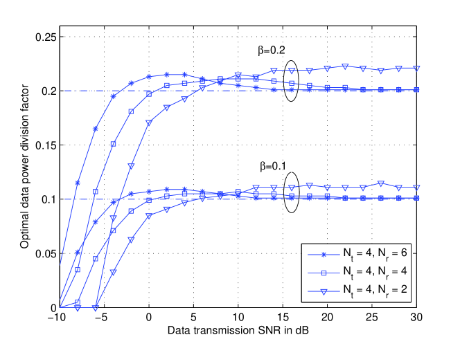
Figure 2: The optimal data power division factor $\phi^{*}$ vs. data transmission SNR $\mathcal{P}_{d}$ for different values of the delay factor $\beta$ and antenna sizes. Perfect channel estimation is assumed.

Fig. 2 shows the optimal data power division factor $\phi^{*}$ given by (24) versus data transmission SNR $\mathcal{P}_{d}$ for different delay factors $\beta$ and antenna sizes assuming perfect channel estimation. It can be seen that $\phi^{*}$ quickly increases from 0 to $\beta$ at very low SNR. For moderate to high SNR, $\phi^{*}$ stays above $\beta$ and converges to $\beta$ as $\mathcal{P}_{d}\rightarrow\infty$. More importantly, we see that $\phi^{*}$ is close to $\beta$ at practical SNR range, e.g., $\mathcal{P}_{d}>0$ dB. Therefore, we conclude that $\phi=\beta$ is a near optimal solution. From (3) we see that $\phi=\beta$ is actually the simplest solution which allocates the same amount of power during each data transmission in both non-adaptive and adaptive sub-blocks, i.e., $\mathcal{P}_{d,1}=\mathcal{P}_{d,2}=\mathcal{P}_{d}$. Furthermore, this simple solution does not require the knowledge of the feedback delay time.

Having $\phi^{*}\approx\beta$ for perfect channel estimation, we argue that $\phi^{*}\approx\beta$ still holds for imperfect channel estimation and will verify its optimality using numerical results. This choice of $\phi$ leads to a simple solution for the optimal PSAM power factor $\alpha^{*}$, as well as the optimal training length $L^{*}_{p}$ for delayed CGF system summarized in Corollary 1, which can be shown by combining the results in Theorem 3, Theorem 4 and those for the non-feedback systems summarized in Section III-A.

Corollary 1

For delayed CGF systems with i.i.d. channels in PSAM schemes, temporally distributing equal power per transmission over both the non-adaptive and adaptive data sub-blocks is a simple and efficient strategy, i.e., $\phi=\beta$. With this strategy, the optimal PSAM power factor $\alpha^{*}$ and the optimal training length $L^{*}_{p}$ coincide with those in the delayless case given in Theorem 3 and 4.

IV-C Numerical Results

Now, we present numerical results to illustrate the capacity gain from optimizing the PSAM power factor. The numerical results also validate the optimality of the transmission strategy in Corollary 1.

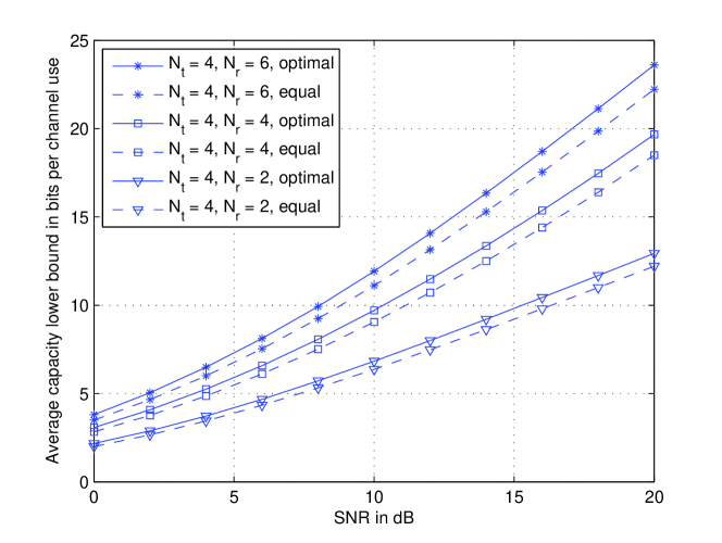
Figure 3: Average capacity lower bound $\overline{C}_{\rm{LB}}$ in (11) vs. SNR $\mathcal{P}$ for delayless CGF systems ($\beta=0$) with i.i.d. channels and different antenna sizes. The block length is $L=100$. Both optimal temporal power allocation to pilot and data as well as equal power allocation are shown for comparison. For optimal temporal power allocation, the training length is $L^{*}_{p}=4$; while for equal power allocation, the pilot length is optimized numerically.

Fig. 3 shows the average capacity lower bound $\overline{C}_{\rm{LB}}$ in (11) versus SNR $\mathcal{P}$ for delayless CGF systems (i.e., $d=0$) with i.i.d. channels and different antenna sizes. The solid lines indicate systems using $\alpha^{*}$ and $L^{*}_{p}$ ($L^{*}_{p}=4$ in this case). The dashed lines indicate systems using equal temporal power allocation and $L^{*}_{p}$ found numerically. Comparing the solid and dashed lines, we see that the capacity gain from optimal temporal power allocation is approximately 9% at 0 dB and 6% at 20 dB for all three systems. This range of capacity gain (5% to 10%) was also observed in [9] for non-feedback systems which can be viewed as an extreme case of delayed CGF system with $d=L_{d}$. From the results for the extreme cases, i.e., $d=0$ and $d=L_{d}$, we conclude that the capacity gain from optimizing the PSAM power factor is around 5% to 10% at practical SNR for delayed CGF systems with i.i.d. channels.

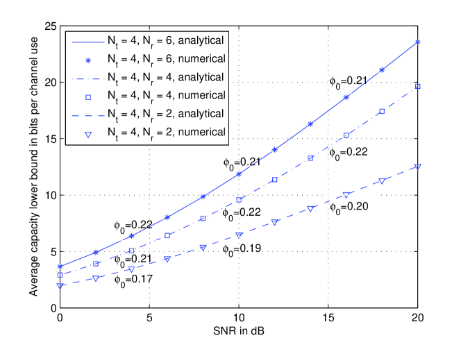
Figure 4: Average capacity lower bound in (11) vs. SNR $\mathcal{P}$ for delayed CGF systems with i.i.d. channels and different antenna sizes. Within a block length of $L=100$, the training length is $L_{p}=4$, followed by a non-adaptive data transmission sub-block of length $d=20$ and an adaptive data transmission sub-block of length $76$. The lines indicate the use of $\phi=\beta=0.208$, and the markers indicate optimal data power division factor found numerically.

We now consider delayed CGF systems to verify Corollary 1. Fig. 4 shows the average capacity lower bound $\overline{C}_{\rm{LB}}$ in (11) versus SNR $\mathcal{P}$ for delayed CGF systems with i.i.d. channels and different antenna sizes. In this example, a transmission block of length $L=100$ consists of a training sub-block of $L_{p}=4$ symbol periods, followed by a non-adaptive data sub-block of $d=20$ symbol periods and an adaptive data sub-block of $L_{d}-d=76$ symbol periods. Therefore, the delay factor $\beta=0.208$. The lines indicate the use of $\phi=\beta$, and the markers indicate optimal data power division found through numerical optimization using $\overline{C}_{\rm{LB}}$ in (11). The values of $\phi^{*}$ for SNR = 4 dB, 10 dB and 16 dB are shown in the figure as well. We see that the capacity difference between the system using $\phi=\beta$ and $\phi=\phi^{*}$ is negligible. That is to say the use of temporal equal power transmission over the entire data block is near optimal for systems with channel estimation errors. We have also confirmed that this trend is valid for a wide range of block lengths (results are omitted for brevity). These results validate Corollary 1.

It is noted that we have assumed the feedback link to be noiseless. When noise is present, capacity that can be achieved by adaptive transmission reduces as the noise in the feedback link increases. The capacity reduction due to corrupted channel gain estimates was studied in [24]. It was shown that the capacity reduction can increase quickly with the noise in the estimated channel gains. Therefore, a reliable feedback scheme which minimizes the noise in the estimated channel gains is important for CGF systems. Furthermore, CGF systems need frequent feedback particularly when the block length is relatively small. This requires a significant amount of feedback overhead in the reverse link (from the receiver to the transmitter), which may cause a direct reduction in the overall information rate, especially when both the forward and the reverse links are operating at the same time, e.g., in cellular systems. Therefore, the CGF scheme may not be appropriate in fast fading environments where the block length is small.

V Channel Covariance Feedback (CCF) Systems

As discussed in the previous subsection, CGF systems require frequent use of feedback due to the rapid change in the channel gains. On the other hand, the statistics of the channel gains change much slower than the channel gains themselves. As a result, it is practical for the receiver to accurately measure the channel covariance matrix and feed it back to the transmitter at a much lower frequency with negligible feedback overhead and delay. Note that for completely i.i.d. channels, there is no need for CCF. In this section, we consider CCF systems with spatially correlated channels and investigate the optimal pilot and data transmission strategy, as well as the optimal power allocation.

V-A Proposed Transmission Scheme

Intuitively, the amount of training resource required for spatially correlated channels should be less than that for i.i.d. channels, as spatial correlation reduces the uncertainty in the channel gains. From [9], we know for i.i.d. channels that the optimal training length $L^{*}_{p}$ equals the number of transmit antennas provided that the optimal PSAM power factor $\alpha^{*}$ is used. Therefore, we expect that $L^{*}_{p}\leq N_{t}$ for correlated channels if we optimize $\alpha$. However, most studies on the optimal pilot design for correlated channels assume $L_{p}\geq N_{t}$ [15, 16, 17]. It was shown in [16] that the optimal training strategy is to train along the eigenvectors of the channel covariance matrix with training power being waterfilled according to the eigenvalues of the channel covariance matrix. Since we expect $L_{p}\leq N_{t}$, we modify the training strategy such that only the $L_{p}$ strongest eigen-channels are trained.

We perform eigenvalue decomposition on $\boldsymbol{R}_{\boldsymbol{H}}$ as $\boldsymbol{R}_{\boldsymbol{H}}=\boldsymbol{U}\boldsymbol{G}{\boldsymbol{U}}^{\dagger}$, and let the eigenvalues of $\boldsymbol{R}_{\boldsymbol{H}}$ be sorted in descending order in $\boldsymbol{g}={[g_{1}\,\,g_{2}\,\,\ldots\,\,g_{N_{t}}]}^{T}$. The optimal training sequence which minimizes the channel estimation errors (i.e., $\text{tr}\{\boldsymbol{R}_{\tilde{\boldsymbol{H}}}\}$) has the property that the eigenvalue decomposition of $\boldsymbol{X}_{p}{\boldsymbol{X}_{p}}^{\dagger}$ is given by $\boldsymbol{X}_{p}{\boldsymbol{X}_{p}}^{\dagger}=\boldsymbol{U}\boldsymbol{P}{\boldsymbol{U}}^{\dagger}$ [16], where $\boldsymbol{P}$ is a diagonal matrix. The entries of $\boldsymbol{P}$ which minimize the channel estimation errors follow a water-filling solution given by

$$p_{i}=\left\{\begin{array}[]{ll}[\mu-g^{-1}_{i}]^{+},\,\,\,\,\,\,i=1,\ldots,L_{p},&\mbox{ with $\sum_{i=1}^{L_{p}}p_{i}=\mathcal{P}_{p}L_{p}$}\\ 0,\,\,\,\,\,\,\,\,\,\,\,\,\,\,i=L_{p}+1,\ldots,N_{t},\end{array}\right.$$ (27)

where $\mu$ is the water level and $\boldsymbol{p}={[p_{1}\,\,p_{2}\,\,\ldots\,\,p_{N_{t}}]}^{T}$ are the eigenvalues of $\boldsymbol{X}_{p}{\boldsymbol{X}_{p}}^{\dagger}$. In practice, the transmitter can ensure that the number of non-zero $p_{i}$ equals $L_{p}$ by changing $L_{p}$ accordingly.

For data transmission, it was shown that the optimal strategy is to transmit along the eigenvectors of $\boldsymbol{R}_{\boldsymbol{H}}$ under the perfect channel estimation [4, 5, 6]. With channel estimation errors, one strategy is to transmit data along the eigenvectors of $\boldsymbol{R}_{\hat{\boldsymbol{H}}}$. With the proposed training sequence, it is easy to show from (6) and (7) that the eigenvectors of $\boldsymbol{R}_{\tilde{\boldsymbol{H}}}$ and $\boldsymbol{R}_{\hat{\boldsymbol{H}}}$ are the same as those of $\boldsymbol{R}_{\boldsymbol{H}}$. Therefore, the eigenvalue decomposition of $\boldsymbol{R}_{\hat{\boldsymbol{H}}}$ can be written as $\boldsymbol{R}_{\hat{\boldsymbol{H}}}=\boldsymbol{U}\hat{\boldsymbol{G}}{\boldsymbol{U}}^{\dagger}$, and we set $\boldsymbol{Q}=\boldsymbol{U}\hat{\boldsymbol{Q}}{\boldsymbol{U}}^{\dagger}$ where $\hat{\boldsymbol{Q}}$ is a diagonal matrix with entries denoted by $q_{i},\,\forall\,i=1,...,N_{t}$.

However, there is no closed-form solution to the optimal spatial power allocation even with perfect channel estimation [4, 5, 6]. Following the proposed training scheme, we propose to transmit data through the $L_{p}$ trained eigen-channels with equal power. That is

$$q_{i}=\left\{\begin{array}[]{ll}\mathcal{P}_{d}/L_{p},\,\,\,\,\,\,i=1,\ldots,L_{p},\\ 0,\,\,\,\,\,\,\,\,i=L_{p}+1,\ldots,N_{t}.\end{array}\right.$$ (30)

For the proposed training and data transmission scheme, the capacity lower bound per channel use in (9) reduces to

$$C_{{\rm{LB}}}\!\!\! = \!\!\!E_{\hat{\boldsymbol{H}}_{0}}\Big{\{}\log_{2}\Big{|}\boldsymbol{I}_{N_{t}}+{\hat{\boldsymbol{H}}_{0}}^{\dagger}\hat{\boldsymbol{H}}_{0}\hat{\boldsymbol{G}}\hat{\boldsymbol{Q}}(1+\mu^{-1}\mathcal{P}_{d})^{-1}\Big{|}\Big{\}},$$ (31)

where the (diagonal) entries of $\hat{\boldsymbol{G}}$ are given by $\hat{g}_{i}=g_{i}-\mu^{-1},\,\forall\,i=1,...,L_{p}$ and $\hat{g}_{i}=0,\,\forall\,i=L_{p}+1,..,N_{t}$, which is derived from (6), (7) and (27).

V-B Optimal Temporal Power Allocation

Now, we investigate the optimal PSAM power factor $\alpha^{*}$ using the capacity lower bound given in (31). The result is summarized in the following theorem.

Theorem 5

For CCF systems in PSAM schemes with the transmission strategy proposed in Section V-A, the optimal PSAM power factor $\alpha^{*}$ is given by (15) with $\gamma=\frac{L_{d}}{L_{d}-L_{p}}$, provided that $\mathcal{P}L\gg\sum_{i=1}^{L_{p}}g^{-1}_{i}$.

Proof: see Appendix E.

Remark: It is noted that $\gamma$ in the optimal solution in Theorem 5 is essentially the same as the one given in Section III-A when $\mathcal{P}L\gg 1$. The condition of $\mathcal{P}L\gg\sum_{i=1}^{L_{p}}g^{-1}_{i}$ can be easily satisfied when the block length is not too small or the SNR is moderate to high (i.e., $\mathcal{P}L\gg 1$), and the spatial correlation between any trained channels is not close to 1. Therefore, the result in Theorem 5 applies to many practical scenarios. It is important to note that the optimal PSAM power factor $\alpha^{*}$ given in Theorem 5 does not depend on the channel spatial correlation, provided the condition is met. In other words, this unique design is suitable for a relatively wide range of channel spatial correlation.

The following steps describe the algorithm for transmission design of CCF systems: 1. For each $L_{p}$ ($L_{p}\leq N_{t}$), design the pilot and data transmission according to Section V-A. 2. Perform temporal power allocation to pilot and data according to Section V-B. 3. Numerically compare the capacity lower bound in (11) for different $L_{p}$ and choose $L^{*}_{p}$ which maximizes the capacity.

V-C A Special Case: Beamforming

Beamforming is a special case of the proposed transmission scheme where only the strongest eigen-channel is used, i.e., $L_{p}=1$. The use of beamforming significantly reduces the complexity of the system as it allows the use of well-established scalar codec technology and only requires the knowledge of the strongest eigen-channel (not the complete channel statistics) [5]. For beamforming transmission, the capacity lower bound in (31) reduces to

$$C_{{\rm{LB}}}\!\!\! = \!\!\!E_{\hat{\boldsymbol{h}}_{0}}\Big{\{}\log_{2}\Big{(}1+{\hat{\boldsymbol{h}}_{0}}^{\dagger}\hat{\boldsymbol{h}}_{0}\frac{(g_{\text{max}}-\mu^{-1})\mathcal{P}_{d}}{1+\mu^{-1}\mathcal{P}_{d}}\Big{)}\Big{\}},$$ (32)

$$= \!\!\!E_{\hat{\boldsymbol{h}}_{0}}\Big{\{}\log_{2}\Big{(}1+{\hat{\boldsymbol{h}}_{0}}^{\dagger}\hat{\boldsymbol{h}}_{0}\frac{g_{\text{max}}\mathcal{P}_{p}\mathcal{P}_{d}}{g^{-1}_{\text{max}}+\mathcal{P}_{p}+\mathcal{P}_{d}}\Big{)}\Big{\}},$$

where $\hat{\boldsymbol{h}}_{0}$ is a $N_{r}\times 1$ vector with i.i.d. ZMCSCG and unit variance entries, $g_{\text{max}}$ is the largest eigenvalue in $\boldsymbol{g}$, and $\mu=\mathcal{P}_{p}+g^{-1}_{\text{max}}$ which can be found by letting $L_{p}=1$ in (27).

Theorem 6

For CCF systems in PSAM schemes with beamforming, the optimal PSAM power factor $\alpha^{*}$ is given in (15) with $\gamma=\frac{1+g_{\text{max}}\mathcal{P}L}{g_{\text{max}}\mathcal{P}L(L-2)/(L-1)}$.

Proof: The proof can be obtained by letting $L_{p}=1$ and $g_{i}=g_{\text{max}}$ in the proof of Theorem 5. $\Box$

Remark: It can be shown for the beamforming case that $\frac{\mathrm{d}\alpha^{*}}{\mathrm{d}g_{\text{max}}}>0$. Therefore, the optimal PSAM power factor $\alpha^{*}$ increases as the channel spatial correlation increases, that is to say, more power should be allocated to data transmission when the channels become more correlated. When $\mathcal{P}L\gg 1$, $\gamma$ reduces to $\frac{L-1}{L-2}$, hence $\alpha^{*}$ does not depend on the channel correlation.

V-D Numerical Results

For numerical analysis, we choose the channel covariance matrix to be in the form of $[\boldsymbol{R}_{\boldsymbol{H}}]_{ij}=\rho^{|i-j|}$, where $\rho$ is referred to as the spatial correlation factor [25, 16]. Our numerical results validate the solution to the optimal PSAM power factor given in Theorem 5 and Theorem 6. The results also show that optimizing the training length can significantly improve the capacity, and the simple transmission scheme proposed in Section V-A gives near optimal performance.

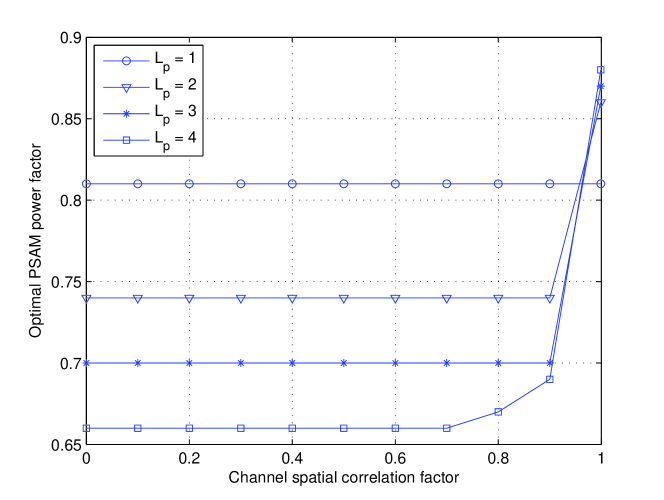
Figure 5: Optimal PSAM power factor $\alpha^{*}$ vs. channel spatial correlation factor $\rho$ for CCF $4\times 4$ systems with a block length of $L=20$ and SNR = 10 dB. All values of $\alpha^{*}$ are found numerically.

Fig. 5 shows the optimal PSAM power factor $\alpha^{*}$ found numerically versus the channel correlation factor $\rho$ for CCF $4\times 4$ systems with a block length of $L=20$ and SNR of 10 dB. We see that $\alpha^{*}$ remains constant before the correlation factor gets close to 1 for $L_{p}>1$, and this value of $\alpha^{*}$ is the same as the analytical value computed from Theorem 5. For the beamforming case where $L_{p}=1$, we see that $\alpha^{*}$ does not depend on the channel correlation, which agrees with our earlier observation from Theorem 6. Similar to CGF systems, we have also compared the capacity achieved using $\alpha^{*}$ and that using equal power allocation over pilot and data, and the same trend is observed (results are omitted for brevity), that is, capacity gain from optimizing PSAM power factor is around 5% to 10% at practical SNR.

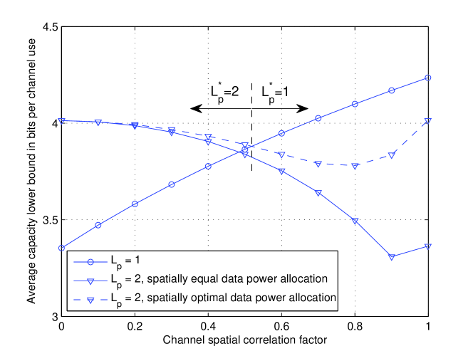
Figure 6: Average capacity lower bound $\overline{C}_{\rm{LB}}$ in (11) vs. channel spatial correlation factor $\rho$ for CCF $2\times 2$ systems with a block length of $L=20$ and SNR of 10 dB. Training length of $L_{p}=1$ and $L_{p}=2$ are shown. For $L_{p}=2$, both spatial equal data power allocation (dashed lines) and optimal data power allocation found numerically (solid lines) are shown.

In our proposed transmission scheme for CCF systems, spatially equal power allocation is used for data transmission. Here we illustrate the optimality of this simple scheme in Fig. 6, which shows the average capacity lower bound $\overline{C}_{\rm{LB}}$ in (11) versus channel correlation factor $\rho$ for CCF $2\times 2$ systems. We compute the capacity achieved using $L_{p}=1$, and $L_{p}=2$ with spatially equal power allocation for data transmission (solid line) and optimal power allocation found numerically (dashed line) for a block length of $L=20$. We also indicate the critical $\rho$ at which $L^{*}_{p}$ changes from 2 to 1 in Fig. 6. It is clear that the capacity loss from spatially optimal power allocation to spatially equal power allocation increases as $\rho$ increases. At the critical $\rho$, this capacity loss is only around 1.5%. We also studied the results for different values of block lengths and the same trend was found (results are omitted for brevity). These results imply that our proposed transmission scheme is very close to optimal provided that the training length is optimized.

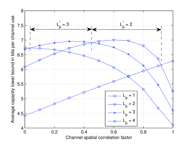
Figure 7: Average capacity lower bound $\overline{C}_{\rm{LB}}$ in (11) vs. channel spatial correlation factor $\rho$ for CCF $4\times 4$ systems with a block length of $L=20$ and SNR = 10 dB. The optimal PSAM power factor $\alpha^{*}$ is used in all results.

Fig. 7 shows the average capacity lower bound $\overline{C}_{\rm{LB}}$ in (11) versus the channel correlation factor $\rho$ for CCF $4\times 4$ systems with a block length of $L=20$ and SNR of 10 dB. The optimal PSAM power factor $\alpha^{*}$ shown in Fig. 5 is used in the capacity computation. Comparing the capacity with different training lengths, we see that $L^{*}_{p}$ decreases as the channel becomes more correlated. More importantly, the capacity gain from optimizing the training length according to the channel spatial correlation can be significant. For example, the capacity at $\rho=0.5$ using $L_{p}=4$ (which is optimal for i.i.d. channels) is approximately 6.3 bits per channel use, while the capacity at $\rho=0.5$ using $L^{*}_{p}=2$ is around 7 bits per channel use, that is to say, optimizing training length results in a capacity improvement of 11% at $\rho=0.5$. Moreover, the capacity improvement increases as channel correlation increases. The same trends are found for different values of block lengths, although the capacity improvement by optimizing the training length reduces as the block length increases (results are omitted for brevity). Therefore, it is important to numerically optimize the training length for correlated channels at small to moderate block lengths.

Furthermore, one can record the range of $\rho$ for each value of $L^{*}_{p}$ from Fig. 7, and observe the value of $\alpha^{*}$ in the corresponding range of $\rho$ in Fig. 5. It can be seen that within the range of $\rho$ where a given $L_{p}$ is optimal, the value of $\alpha^{*}$ for the given $L_{p}$ is a constant given by Theorem 5 provided that $\mathcal{P}L\gg 1$. That is to say, the condition in Theorem 5 (i.e., $\mathcal{P}L\gg\sum_{i=1}^{L_{p}}g^{-1}_{i}$) can be simplified to $\mathcal{P}L\gg 1$ provided that the training length is optimized.

V-E Hybrid CGF and CCF Systems

After studying the optimal transmission and power allocation strategy for CGF systems with i.i.d. channels and CCF system with correlated channels, we provide some discussion on systems utilizing both CGF and CCF with correlated channels. For spatially correlated channels, the optimal training follows a water-filling solution according to the channel covariance, and the optimal data transmission follows a water-filling solution according to the estimated channel gains. The two different water-filling solutions make the problem of optimizing the PSAM power factor mathematically intractable. Furthermore, the optimal training length $L^{*}_{p}$ may be smaller than the number of transmit antennas, and needs to be found numerically. However, from the results for CGF systems with i.i.d. channels in Section IV and CCF system with correlated channel in Section V, one may expect that a good solution for the optimal PSAM power factor $\alpha^{*}$ in the hybrid system is given in Theorem 5.

VI Summary of Results

In this paper, we have studied block fading MIMO systems with feedback in PSAM transmission schemes. Two typical feedback systems are considered, namely the channel gain feedback and the channel covariance feedback systems. Using an accurate capacity lower bound as the figure of merit, we have provided the solutions for the optimal power allocation to training and data transmission as well as the optimal training length. Table I summarizes the design guidelines for both non-feedback systems and feedback systems.

TABLE I: Summary of Design Guidelines

System	Channel	Design Guidelines	Reference
	i.i.d.	$\bullet\,$Transmit orthogonal pilots among antennas with spatially equal power.	[2, 9]
Non-		$\bullet\,$Transmit independent data among antennas with spatially equal power.
feedback		$\bullet\,$The optimal PSAM power factor $\alpha^{*}$ is given by (15) with $\gamma=\frac{N_{t}+\mathcal{P}L}{\mathcal{P}L(1-N_{t}/L_{d})}$.
		$\bullet\,$The optimal training length $L^{*}_{p}$ equals the number of transmit antennas $N_{t}$.
	correlated	$\bullet\,$Use the designs for i.i.d. channels as a robust choice.	Sec. III-B
CGF	i.i.d.	$\bullet\,$Transmit orthogonal pilots with spatially equal power.	Sec. IV
		$\bullet\,$Transmit independent data with spatially equal power in data sub-block 1
		and spatial power water-filling in data sub-block 2 (see Fig. 1).
		$\bullet\,$Distribute equal power per transmission throughout data sub-blocks 1 and 2.
		$\bullet\,$$\alpha^{*}$ and $L^{*}_{p}$ for non-feedback system are (near) optimal for (delayed) CGF system.
CCF	correlated	$\bullet\,$For a given $L_{p}$ ($L_{p}\leq N_{t}$), transmit pilots along the $L_{p}$ strongest	Sec. V
		eigen-channels with spatial power water-filling according to (27).
		$\bullet\,$Transmit data along the $L_{p}$ trained eigen-channels with spatially equal power.
		$\bullet\,$$\alpha^{*}$ is given by (15) with $\gamma=\frac{L_{d}}{L_{d}-L_{p}}$, provided that $\mathcal{P}L\gg\sum_{i=1}^{L_{p}}g^{-1}_{i}$.
		$\bullet\,$$L^{*}_{p}$ should be numerically optimized.
		$\bullet\,$For beamforming (i.e., $L_{p}=1$), $\alpha^{*}$ is given by (15) with $\gamma=\frac{1+g_{\text{max}}\mathcal{P}L}{g_{\text{max}}\mathcal{P}L(L-2)/(L-1)}$.

Appendix A A Measure of Channel Spatial Correlation

A vector $\boldsymbol{a}={[a_{1}\,\,a_{2}\,\,\ldots\,\,a_{n}]}^{T}$ is said to be majorized by another vector $\boldsymbol{b}={[b_{1}\,\,b_{2}\,\,\ldots\,\,b_{n}]}^{T}$ if

$$\sum_{i=1}^{k}a_{i}\!\leq\!\sum_{i=1}^{k}b_{i},\,\,\,\,k=1,\ldots,n-1,\,\,\,\,\,\,\text{and}\,\,\,\,\sum_{i=1}^{n}a_{i}\!=\!\sum_{i=1}^{n}b_{i},$$ (33)

where the elements in both vectors are sorted in descending order [26]. We denote the relationship as $\boldsymbol{a}\prec\boldsymbol{b}$. Any real-valued function $\Phi$, defined on a vector subspace, is said to be Schur-convex, if $\boldsymbol{a}\prec\boldsymbol{b}$ implies $\Phi(\boldsymbol{a})\leq\Phi(\boldsymbol{b})$ [26]. Similarly $\Phi$ is Schur-concave, if $\boldsymbol{a}\prec\boldsymbol{b}$ implies $\Phi(\boldsymbol{a})\geq\Phi(\boldsymbol{b})$. Following [20], we have the following definition:

Definition 1

Let $\boldsymbol{a}$ contain the eigenvalues of a channel covariance matrix such as $\boldsymbol{R}_{\boldsymbol{a}}$, and $\boldsymbol{b}$ contain the eigenvalues of another channel covariance matrix $\boldsymbol{R}_{\boldsymbol{b}}$. The elements in both vectors are sorted in descending order. Then $\boldsymbol{R}_{\boldsymbol{a}}$ is less correlated than $\boldsymbol{R}_{\boldsymbol{b}}$ if and only if $\boldsymbol{a}\prec\boldsymbol{b}$.

Appendix B Proof of Theorem 1

This is a max-min problem where the MSE of the channel estimates is to be minimized by $\boldsymbol{X}_{p}{\boldsymbol{X}_{p}}^{\dagger}$ and to be maximized by $\boldsymbol{R}_{\boldsymbol{H}}$. We need to show that $\text{inf}_{\boldsymbol{X}_{p}{\boldsymbol{X}_{p}}^{\dagger}}\,\,\text{sup}_{\boldsymbol{R}_{\boldsymbol{H}}}\,\text{tr}\{\boldsymbol{R}_{\tilde{\boldsymbol{H}}}\}$ is achieved by orthogonal pilot sequence with equal power allocated among the transmit antennas, i.e., $\boldsymbol{X}_{p}{\boldsymbol{X}_{p}}^{\dagger}=\frac{\mathcal{P}_{p}L_{p}}{N_{t}}\boldsymbol{I}_{N_{t}}$, assuming $L_{p}\geq N_{t}$.

From (6) we see that

$$\text{sup}_{\boldsymbol{R}_{\boldsymbol{H}}}\,\text{tr}\{\boldsymbol{R}_{\tilde{\boldsymbol{H}}}\} \geq \text{tr}\{(\boldsymbol{I}_{N_{t}}+\boldsymbol{X}_{p}{\boldsymbol{X}_{p}}^{\dagger})^{-1}\}=\sum_{i=1}^{N_{t}}(1+p_{i})^{-1},$$ (34)

where $\boldsymbol{p}={[p_{1}\,\,p_{2}\,\,\ldots\,\,p_{N_{t}}]}^{T}$ are the eigenvalues of $\boldsymbol{X}_{p}{\boldsymbol{X}_{p}}^{\dagger}$. Since the sum of a convex function of $p_{i}$ is Schur-convex in $\boldsymbol{p}$ [26], we conclude that (34) is Schur-convex in $\boldsymbol{p}$. Since $\text{tr}\{\boldsymbol{X}_{p}{\boldsymbol{X}_{p}}^{\dagger}\}=\mathcal{P}_{p}L_{p}$, we have

$$\text{sup}_{\boldsymbol{R}_{\boldsymbol{H}}}\,\text{tr}\{\boldsymbol{R}_{\tilde{\boldsymbol{H}}}\} \geq \sum_{i=1}^{N_{t}}\Big{(}1+\frac{\mathcal{P}_{p}L_{p}}{N_{t}}\Big{)}^{-1},$$ (35)

where we have used $\boldsymbol{X}_{p}{\boldsymbol{X}_{p}}^{\dagger}=\frac{\mathcal{P}_{p}L_{p}}{N_{t}}\boldsymbol{I}_{N_{t}}$. Note that (35) holds for any $\boldsymbol{X}_{p}{\boldsymbol{X}_{p}}^{\dagger}$. On the other hand

$$\text{inf}_{\boldsymbol{X}_{p}{\boldsymbol{X}_{p}}^{\dagger}}\,\,\text{sup}_{\boldsymbol{R}_{\boldsymbol{H}}}\,\text{tr}\{\boldsymbol{R}_{\tilde{\boldsymbol{H}}}\} \leq \,\,\text{sup}_{\boldsymbol{R}_{\boldsymbol{H}}}\,\text{tr}\Big{\{}\Big{(}\boldsymbol{R}_{\boldsymbol{H}}^{-1}+\frac{\mathcal{P}_{p}L_{p}}{N_{t}}\boldsymbol{I}_{N_{t}}\Big{)}^{-1}\Big{\}},$$ (36)

$$= \,\,\text{sup}_{\boldsymbol{R}_{\boldsymbol{H}}}\,\sum_{i=1}^{N_{t}}\Big{(}g^{-1}_{i}+\frac{\mathcal{P}_{p}L_{p}}{N_{t}}\Big{)}^{-1},$$

$$\leq \sum_{i=1}^{N_{t}}\Big{(}1+\frac{\mathcal{P}_{p}L_{p}}{N_{t}}\Big{)}^{-1},$$

where (36) is obtained using the Schur-concavity of $\sum_{i=1}^{N_{t}}\Big{(}g^{-1}_{i}+\frac{\mathcal{P}_{p}L_{p}}{N_{t}}\Big{)}^{-1}$ in $\boldsymbol{g}$. From (35) and (36), we conclude that

$$\text{inf}_{\boldsymbol{X}_{p}{\boldsymbol{X}_{p}}^{\dagger}}\,\,\text{sup}_{\boldsymbol{R}_{\boldsymbol{H}}}\,\text{tr}\{\boldsymbol{R}_{\tilde{\boldsymbol{H}}}\} = \sum_{i=1}^{N_{t}}\Big{(}1+\frac{\mathcal{P}_{p}L_{p}}{N_{t}}\Big{)}^{-1},$$

which can be achieved by $\boldsymbol{X}_{p}{\boldsymbol{X}_{p}}^{\dagger}=\frac{\mathcal{P}_{p}L_{p}}{N_{t}}\boldsymbol{I}_{N_{t}}$. $\Box$

Appendix C Proof of Theorem 3

Figure 8: A sketch example of $\rho_{\text{eff}}$ v.s. $\alpha$. The vertical dashed lines indicates the values of $\alpha$ at which $m$ changes its value. $\alpha_{1}$, $\alpha_{2}$, $\alpha_{3}$ and $\alpha_{4}$ indicate the local optimal values of $\alpha$ which gives local maximal $\rho_{\text{eff}}$.

With $\sigma^{2}_{\tilde{\boldsymbol{H}}}=\Big{(}1+\frac{\mathcal{P}_{p}L_{p}}{N_{t}}\Big{)}^{-1}$, $\sigma^{2}_{\hat{\boldsymbol{H}}}=1-\sigma^{2}_{\tilde{\boldsymbol{H}}}$ and (2), it can be shown that $\rho_{\text{eff}}\triangleq\frac{\sigma^{2}_{\hat{\boldsymbol{H}}}\mathcal{P}_{d}}{1+\sigma^{2}_{\tilde{\boldsymbol{H}}}\mathcal{P}_{d}}$ is a concave function of $\alpha\in[0,1]$. Also, $m$ is discrete and non-decreasing on $\alpha\in[0,1]$ as the number of active eigen-channel cannot decrease as the data transmission power increases. Here we show a sketch plot of $\rho_{\text{eff}}$ versus $\alpha$ in Fig. 8 to visualize the proof. From (19) we see that $C_{{\rm{LB}}}$ is maximized when $\rho_{\text{eff}}$ reaches its maximum for any fixed $m$. Therefore, we will have $\alpha^{*}_{1}$, $\alpha^{*}_{2}$, $\alpha^{*}_{3}$ and $\alpha^{*}_{4}$ as the local optimal points in Fig. 8 which maximize $C_{{\rm{LB}}}$ in corresponding regions of $\alpha$. From the property of water-filling solution in (17), we know that $q_{i}$ is continuous on $\mathcal{P}_{d}$ and hence, is continuous on $\alpha\in[0,1]$. Therefore, $C_{{\rm{LB}}}$ in (16) is continuous on $\alpha\in[0,1]$. This implies that $C_{{\rm{LB}}}$ is continuous across the boundaries of different regions of $\alpha$, indicated by the dashed lines in Fig. 8. Consequently, the global optimal point $\alpha^{*}_{3}=\alpha^{*}$ which maximizes $\rho_{\text{eff}}$ in Fig. 8 is also the global optimal point which maximizes $C_{{\rm{LB}}}$. It is noted that the objective function $\rho_{\text{eff}}$ is the same as that in non-feedback systems given in [9]. Therefore, the solution of $\alpha^{*}$ coincides with the solution for non-feedback systems given in (15). $\Box$

Appendix D Proof of Theorem 4

We let $\rho_{\text{eff}}\triangleq\frac{\sigma^{2}_{\hat{\boldsymbol{H}}}\mathcal{P}_{d}}{1+\sigma^{2}_{\tilde{\boldsymbol{H}}}\mathcal{P}_{d}}$, $y=\sum_{i=1}^{m}\ln\frac{\lambda_{i}}{m}$, and $z=\sum_{i=1}^{m}\lambda^{-1}_{i}$. Then the average capacity lower bound in (11) can be rewritten using (19) as

$$\overline{C}_{\rm{LB}} = \frac{L_{d}}{L}\frac{1}{\ln 2}E_{\boldsymbol{\lambda}}\{m\ln(\rho_{\text{eff}}+z)+y\}.$$

Differentiating $\overline{C}_{\rm{LB}}$ w.r.t., $L_{d}$ for any fixed $m$ gives

$$\frac{\mathrm{d}\overline{C}_{\rm{LB}}}{\mathrm{d}L_{d}} = \frac{1}{\ln 2}\frac{m}{L}\Big{(}E_{\boldsymbol{\lambda}}\Big{\{}\ln(\rho_{\text{eff}}+z)+\frac{L_{d}}{\rho_{\text{eff}}+z}\frac{\mathrm{d}\rho_{\text{eff}}}{\mathrm{d}L_{d}}+\frac{y}{m}\Big{\}}\Big{)}.$$ (37)

Similar to [9], we need to show that $\frac{\mathrm{d}\overline{C}_{\rm{LB}}}{\mathrm{d}L_{d}}>0$. It can be shown that $\overline{C}_{\rm{LB}}$ is continuous on $L_{d}$ (treating $L_{d}$ as a positive real-valued variable) regardless the value of $m$. Therefore, the value of $m$ does not cause any problem in the proof.

Here we consider the case where $L_{d}>N_{t}$ and omit the cases $L_{d}=N_{t}$ and $L_{d}<N_{t}$ which can be handled similarly. Taking the derivative of $\rho_{\text{eff}}$ w.r.t., $L_{d}$ with some algebraic manipulation, we have

$$\frac{\mathrm{d}\rho_{\text{eff}}}{\mathrm{d}L_{d}} = -\frac{\rho_{\text{eff}}}{L_{d}-N_{t}}\left(1-\sqrt{\frac{N_{t}(N_{t}+\mathcal{P}L)}{L_{d}(L_{d}+\mathcal{P}L)}}\right).$$ (38)

Substituting (38) into (37), we get

$$\frac{\mathrm{d}\overline{C}_{\rm{LB}}}{\mathrm{d}L_{d}}\!\!\! = \!\!\!\frac{1}{\ln 2}\frac{m}{L}\left(E_{\boldsymbol{\lambda}}\Big{\{}\ln(\rho_{\text{eff}}+z)-\frac{\rho_{\text{eff}}}{\rho_{\text{eff}}+z}\frac{L_{d}}{L_{d}-N_{t}}\left(1-\sqrt{\frac{N_{t}(N_{t}+\mathcal{P}L)}{L_{d}(L_{d}+\mathcal{P}L)}}\right)+\frac{y}{m}\Big{\}}\right).$$

With $L_{d}>N_{t}$, it can be shown that

$$\frac{L_{d}}{L_{d}-N_{t}}\left(1-\sqrt{\frac{N_{t}(N_{t}+\mathcal{P}L)}{L_{d}(L_{d}+\mathcal{P}L)}}\right)<1.$$

Therefore, it suffices to show that

$$E_{\boldsymbol{\lambda}}\Big{\{}\ln(\rho_{\text{eff}}+z)-\frac{\rho_{\text{eff}}}{\rho_{\text{eff}}+z}+\frac{y}{m}\Big{\}}\geq 0.$$ (39)

Furthermore, one can show that

$$\frac{\mathrm{d}}{\mathrm{d}\rho_{\text{eff}}}E_{\boldsymbol{\lambda}}\Big{\{}\ln(\rho_{\text{eff}}+z)-\frac{\rho_{\text{eff}}}{\rho_{\text{eff}}+z}+\frac{y}{m}\Big{\}}=\frac{\rho_{\text{eff}}}{(\rho_{\text{eff}}+z)^{2}}\geq 0$$

for any fixed $m$. Therefore, we only need to show (39) holds at $\rho_{\text{eff}}=0$, that is

$$E_{\boldsymbol{\lambda}}\Big{\{}\ln z+\frac{y}{m}\Big{\}} = E_{\boldsymbol{\lambda}}\Big{\{}\ln\sum_{i=1}^{m}\lambda^{-1}_{i}+\frac{1}{m}\sum_{i=1}^{m}\ln\frac{\lambda_{i}}{m}\Big{\}},$$

$$\geq E_{\boldsymbol{\lambda}}\Big{\{}\frac{1}{m}\sum_{i=1}^{m}\ln\frac{\lambda^{-1}_{i}}{m}+\frac{1}{m}\sum_{i=1}^{m}\ln\frac{\lambda_{i}}{m}\Big{\}},$$

$$= E_{\boldsymbol{\lambda}}\Big{\{}\ln\frac{\lambda^{-1}_{i}}{m}\frac{\lambda_{i}}{m}\Big{\}}=0,$$

where (D) is obtained using the concavity of $\ln(\cdot)$. Therefore, we conclude that $\frac{\mathrm{d}\overline{C}_{\rm{LB}}}{\mathrm{d}L_{d}}>0$, which implies the training length should be kept minimum, i.e., $L^{*}_{p}=N_{t}$. $\Box$

Appendix E Proof of Theorem 5

For any positive definite matrix $\boldsymbol{A}$, $\log_{2}|\boldsymbol{A}|$ is increasing in $\boldsymbol{A}$ [26]. Also, for any positive semi-definite matrix $\boldsymbol{B}$, $\boldsymbol{I}+{\hat{\boldsymbol{H}}_{0}}^{\dagger}\hat{\boldsymbol{H}}_{0}\boldsymbol{B}$ is a positive definite matrix [2]. Since $\hat{\boldsymbol{G}}\hat{\boldsymbol{Q}}(1+\mu^{-1}\mathcal{P}_{d})^{-1}$ is a positive semi-definite matrix, the capacity lower bound in (31) is maximized when the diagonal entries of $\hat{\boldsymbol{G}}\hat{\boldsymbol{Q}}(1+\mu^{-1}\mathcal{P}_{d})^{-1}$ are maximized.

The $i$th non-zero diagonal entry of $\hat{\boldsymbol{G}}\hat{\boldsymbol{Q}}(1+\mu^{-1}\mathcal{P}_{d})^{-1}$ is given by

$$\rho_{\text{eff},i} = \frac{(g_{i}-\mu^{-1})\mathcal{P}_{d}}{(1+\mu^{-1}\mathcal{P}_{d})L_{p}}=\frac{g_{i}}{L_{p}}\frac{\mathcal{P}_{p}\mathcal{P}_{d}+\mathcal{P}_{d}(y-g^{-1}_{i})}{\mathcal{P}_{p}+\mathcal{P}_{d}+y},$$ (41)

where we have used (27) and let $y=\mu-\mathcal{P}_{p}=\frac{1}{L_{p}}\sum_{i=1}^{L_{p}}g^{-1}_{i}$. Substituting $\alpha$ from (2) into (41) with some algebraic manipulation, we get

$$\rho_{\text{eff},i} = \frac{g_{i}\mathcal{P}L}{L_{p}(L_{d}-L_{p})}\frac{\alpha(1-\alpha)+\alpha\frac{L_{p}}{\mathcal{P}L}(y-g^{-1}_{i})}{-\alpha+\frac{\mathcal{P}L+L_{p}y}{\mathcal{P}L(1-L_{p}/L_{d})}}.$$ (42)

Here we consider the case where $L_{d}>L_{p}$ and omit the cases $L_{d}=L_{p}$ and $L_{d}<L_{p}$ which can be handled similarly. It can be shown that $\rho_{\text{eff},i}$ in (42) is concave in $\alpha\in(0,1)$. Therefore, the optimal $\alpha$ occurs at $\frac{\mathrm{d}\rho_{\text{eff},i}}{\mathrm{d}\alpha}=0$, which is the root to $\alpha^{2}-2\alpha\gamma+\gamma+\gamma z=0$, where $\gamma=\frac{\mathcal{P}L+L_{p}y}{\mathcal{P}L(1-L_{p}/L_{d})}$ and $z=\frac{L_{p}}{\mathcal{P}L}(y-g^{-1}_{i})$. It is clear that $\alpha$ depends on $g_{i}$ through $z$. Therefore, there is no unique $\alpha$ which maximizes all $\rho_{\text{eff},i}$. However, this dependence disappears when $\mathcal{P}L\gg L_{p}y=\sum_{i=1}^{L_{p}}g^{-1}_{i}$. Under this condition, one can show that $\gamma\approx\frac{L_{d}}{L_{d}-L_{p}}$ and $z\approx 0$. And there exists a unique solution of $\alpha^{*}$ which maximizes all the diagonal entries of $\hat{\boldsymbol{G}}\hat{\boldsymbol{Q}}(1+\mu^{-1}\mathcal{P}_{d})^{-1}$, given by

$$\alpha^{*} = \gamma-\sqrt{\gamma(\gamma-1)},\,\,\,\text{where}\,\,\,\gamma=\frac{L_{d}}{L_{d}-L_{p}}.\,\,\,\Box$$

References

- [1] G. J. Foschini and M. J. Gans, “On the limits of wireless communications in a fading environment when using multiple antennas,” Wireless Pers. Commun., vol. 6, no. 3, pp. 311–335, Mar. 1998.
- [2] I. E. Telatar, “Capacity of multi-antenna Gaussian channels,” Eur. Trans. Telecomm., vol. 10, no. 6, pp. 585–595, Nov. 1999.
- [3] T. M. Cover and J. A. Thomas, Elements of Information Theory, 2nd ed. New Jersey: Wiley, 2006.
- [4] E. Visotsky and U. Madhow, “Space-time transmit precoding with imperfect feedback,” IEEE Trans. Inform. Theory, vol. 47, no. 6, pp. 2632–2639, Sept. 2001.
- [5] S. A. Jafar and A. Goldsmith, “Transmitter optimization and optimality of beamforming for multiple antenna systems,” IEEE Trans. Wireless Commun., vol. 3, no. 4, pp. 1165–1175, July 2004.
- [6] E. A. Jorswieck and H. Boche, “Channel capacity and capacity-range of beamforming in MIMO wireless systems under correlated fading with covariance feedback,” IEEE Trans. Wireless Commun., vol. 3, no. 5, pp. 1543–1553, Sept. 2004.
- [7] J. C. Roh and B. D. Rao, “Multiple antenna channels with partial channel state information at the transmitter,” IEEE Trans. Wireless Commun., vol. 3, no. 2, pp. 677–688, Mar. 2004.
- [8] J. Li and Q. T. Zhang, “Transmitter optimization for correlated MISO fading channels with generic mean and covariance feedback,” IEEE Trans. Wireless Commun., vol. 7, no. 9, pp. 3312–3317, Sept. 2008.
- [9] B. Hassibi and M. Hochwald, “How much training is needed in multiple-antenna wireless links?” IEEE Trans. Inform. Theory, vol. 49, no. 4, pp. 951–963, Apr. 2003.
- [10] T. Yoo and A. Goldsmith, “Capacity and power allocation for fading MIMO channels with channel estimation error,” IEEE Trans. Inform. Theory, vol. 52, no. 5, pp. 2203–2214, May 2006.
- [11] S. M. Redl, M. K. Weber, and M. W. Oliphan, An introduction to GSM, 1st ed. Boston: Artech House, 1995.
- [12] J. K. Cavers, “An analysis of pilot symbol assisted modulation for Rayleigh fading channels,” IEEE Trans. Veh. Technol., vol. 40, no. 4, pp. 686–693, Nov. 1991.
- [13] V. Pohl, P. H. Nguyen, V. Jungnickel, and C. Helmolt, “Continuous flat-fading MIMO channels: Achievable rate and optimal length of the training and data phases,” IEEE Trans. Wireless Commun., vol. 4, no. 4, pp. 1889–1900, July 2005.
- [14] X. Zhou, T. A. Lamahewa, P. Sadeghi, and S. Durrani, “Designing PSAM schemes: how optimal are SISO pilot parameters for spatially correlated SIMO?” in Proc. IEEE PIMRC, Sept. 2008.
- [15] J. H. Kotecha and A. M. Sayeed, “Transmit signal design for optimal estimation of correlated MIMO channels,” IEEE Trans. Signal Processing, vol. 52, no. 2, pp. 546–557, Feb. 2004.
- [16] M. Biguesh and A. B. Gershman, “Training-based MIMO channel estimation: a study of estimator tradeoffs and optimal training signals,” IEEE Trans. Signal Processing, vol. 54, no. 3, pp. 884–893, Mar. 2006.
- [17] J. Pang, J. Li, L. Zhao, and Z. Lu, “Optimal training sequences for MIMO channel estimation with spatial correlation,” in Proc. IEEE VTC, Oct. 2007, pp. 651–655.
- [18] J. Pang, J. Li, and L. Zhao, “Optimal training length for MIMO systems with transmit antenna correlation,” in Proc. IEEE WCNC, Mar. 2008, pp. 425–429.
- [19] C. Chuah, D. Tse, J. Kahn, and R. Valenzuela, “Capacity scaling in MIMO wireless systems under correlated fading,” IEEE Trans. Inform. Theory, vol. 48, no. 3, pp. 637–650, Mar. 2002.
- [20] E. A. Jorswieck and H. Boche, “Optimal transmission strategies and impact of correlation in multiantenna systems with different types of channel state information,” IEEE Trans. Signal Processing, vol. 52, no. 12, pp. 3440–3453, Dec. 2004.
- [21] S. M. Kay, Fundamentals of Statistical Signal Processing: Estimation Theory. Prentice hall, 1993.
- [22] X. Zhou, T. A. Lamahewa, P. Sadeghi, and S. Durrani, “Capacity of MIMO systems: Impact of spatial correlation with channel estimation errors,” in Proc. IEEE ICCS, Nov. 2008.
- [23] S. Boyd and L. Vandenberghe, Convex Optimization, 1st ed. Cambridge: Cambridge University Press, 2004.
- [24] E. Baccarelli, M. Biagi, and C. Pelizzoni, “On the information throughput and optimized power allocation for MIMO wireless systems with imperfect channel estimation,” IEEE Trans. Signal Processing, vol. 53, no. 7, pp. 2335–2347, July 2005.
- [25] T. Yoo, E. Yoon, and A. Goldsmith, “MIMO capacity with channel uncertainty: Does feedback help?” in Proc. IEEE Globecom., vol. 1, May 2004, pp. 96–100.
- [26] A. W. Marshall and I. Olkin, Inequalities: Theory of Majorization and Its Applications. Academic Press, 1979.