Preprint PNPI-2795, 2009


Resonance capture by hydrogenous impurities and losses of ultracold neutrons in solid material traps

The capture of trapped ultracold neutrons (UCNs) by closed hydrogenous impurities within a solid coating of the trap is discussed as a possible cause of observed anomalously large losses of UCNs in solid material UCN traps. Then significant losses of UCNs arise only if resonances occur in the UCN-impurity scattering amplitude. For a large size impurity, higher partial waves in the UCN-impurity interaction are important, and they are taken into account in the present paper. The method of the calculation is applicable to irregular shape impurities as well. A small distortion of an impurity shape, if it splits the resonance, can increase the UCN losses by a few times. UCN losses in the beryllium trap are calculated assuming they are due to the UCN capture by ice spherical impurities within the coating of the trap walls. Both s- and p-wave resonances contribute significantly to the UCN losses considered. As an example, observed anomalous large UCN losses are achieved if the average radius of the impurity is about 600 Å  and the impurity density is about $3\times 10^{14}$/cm³. A distortion of the spherical shape of the impurity could increase the UCN losses and therefore decrease the impurity density.

1 Introduction

Losses of ultracold neutrons (UCNs) in material traps have attracted attention in recent years [1]. The matter arises for crystal materials such as beryllium and graphite [1, 2, 3] especially for beryllium [1, 2]. For a liquid or solid Fomblin oil the observed losses could be explained by inelastic scattering processes [4], but it can not [1, 3, 4, 5] explain the UCN losses in beryllium traps. Indeed, the UCN losses in beryllium traps depend slowly on the temperature $T$ at low temperature [1, 2, 3]. By contrast, the inelastic scattering should lead to a $\sim T^{3}$ dependence of the UCN losses. The discussed losses cannot be a result of a surface heating caused by hydrogenous surface impurities [1] because it requires too high a concentration of the hydrogen on the surface. In addition, in this case the losses should be significantly reduced by a degassing procedure, but the observed UCN ones are insensitive to it [1, 2, 3]. The discussed UCN losses cannot be from a coherent absorption of UCN by beryllium because the UCN capture cross section for beryllium is too small. The scattering of UCNs by vacuum cavities can increase the UCN losses [6], but it can hardly explain the anomalously large losses observed [1, 2].

In the present paper we consider UCN losses from the UCN capture by closed impurities within the solid coating of the trap walls. A low temperature of the trap is assumed so that only the elastic scattering and capture of UCNs can take place. Ice impurities are mainly kept in mind because the neutron-hydrogen capture cross section is large. Water within a closed cavity can hardly be removed by a degassing procedure. So losses are insensitive to the degassing process and do not depend on the trap temperature, nearly as it has been observed experimentally.

A possible correlation of large losses of UCNs in beryllium with incoherent processes has been noted in [1, 7]. In [1] the concept of a localization of UCNs around the lattice defect has been proposed which drasticly increases the UCN losses. This mechanism of UCN losses is not, however, acceptable since it is based on a mistakable solution of the scattering problem [8].

At low temperatures the losses of UCNs arise solely when absorption of UCNs takes place. If UCN losses are due to coherent absorption of UCN by the medium, then the well known expression [6] for the coefficient $\mu(y)$ of the UCN losses is as follows:

$$\mu(y)=\frac{2\eta}{y^{2}}(\arcsin y-y\sqrt{1-y^{2}}),\quad y=\sqrt{E/U^{\prime}}\,,$$ (1)

where $E$ is the UCN energy, $U^{\prime}$ is the real part of the optical potential, and $\eta=U^{\prime\prime}/U^{\prime}$, where $U^{\prime\prime}$ is the imaginary part of the optical potential of the medium. Inelastic scattering is negligible at low temperatures and so $\eta=b^{\prime}/b$, where $b^{\prime}$ is the UCN absorption amplitude and $b$ is the UCN elastic scattering amplitude. Then for beryllium $\eta=2.47\times 10^{-7}$ while the experimental losses [1] require $\eta=3\times 10^{-5}$. This exceeds the expected value of $\eta$ by a factor of about 100. The UCN losses due to UCN capture by a small size impurity are again represented by (1) with the understanding that $\eta$ is replaced by $p_{V}w$ where $p_{V}$ is the portion of the total volume occupied by impurities, and $w=W/U^{\prime}$. Here $(-W)$ is the imaginary part of the UCN- impurity potential. For hydrogen $w$ is known to be $w\approx 3\times 10^{-6}$. Then $\eta\sim 10^{-5}$ requires $p_{V}\sim 10$ which is an obviously unacceptable result.

The losses drastically grow for a large size impurity when a resonance in the UCN-impurity scattering amplitude occurs. Compared with the UCN losses by a vacuum cavity [6], they are increased by a factor, which roughly is $wa\kappa U^{\prime}/(E\eta)$. In this case $a$ is the radius of the impurity and $\kappa=\sqrt{2m(U-E)/\hbar^{2}}$ is the length of the UCN penetration into the coating; $m$ is the neutron mass and $\hbar$ is the Plank constant (reduced). Under the discussed conditions this factor is $\sim 100$.

As is shown in the paper, a relatively small impurity shape distortion, which splits the resonance into $N$ resonances, increases the UCN losses, roughly, by N times. In particular, a small distortion of the spherical impurity is able to increases the UCN losses from the $l$-wave resonance by about $(2l+1)$ times in comparison with the UCN losses from a spherical impurity occupying the same volume. In the paper, however, as the first step, spherical shape impurities are mainly considered.

Computations are performed under conditions where experimental data of the UCN losses are obtained [1]. Then the maximal UCN energy in the trap is about 23 cm, 38 cm, 46 cm, 52 cm and 58 cm (this means that the UCN energy is the same as the gravitational energy of the neutron lifted to the given height; 1 cm energy corresponds to $1.025\times 10^{-9}$ eV). The radius of ice impurity is taken in the range (453.7 – 875.2) Å. If the radius is less than 464.2 Å, then a resonance does not occur for the UCN energy below 58 cm, and such size impurities do not contribute to the UCN losses. In the radius range being approximately (460–740) Å, only an s-wave resonance occurs, and solely the s-wave UCN-impurity interaction is important. If the radius is larger than 740 Å, then both s- and p-wave interactions contribute to the UCN losses. The $s-p$ wave interference is taken into account, too. The UCN losses mainly arise from impurities lying rather far from the trap wall, but not from those lying on the trap surface. The d-wave interaction is negligible since a $d$-wave resonance does not occur in the discussed energy-radius region.

When an $l$-wave resonance is present, then the $l$-wave nonresonance background grows and contributes about (20–30)$\%$ to the UCN losses. Therefore a resonance approximation such as that employed in [6] is not used in the above computations. A large radius approximation [6] is not used in above computations, too. Nevertheless, both these approximations are discussed (in Sec. IV) for a semiquantitative consideration of the matter.

An example of the distribution of the ice impurities is proposed fitting the experimental data [1]. Now experimental data are insufficient to fit them in the unique way. It assumes that no impurities have radii greater than 875 Å. The impurity density is required to be about $3\times 10^{14}$/cm³. In fact the density falls when the size of the impurity increases. As a result, the average size of the impurity is about 600 Å. The impurities occupy 0.25 of the total volume. This is rather a large part of the volume, but not so much that the UCN capture by hydrogenous impurities should be discarded as a possible cause of the UCN losses. Perhaps, in accordance with aforesaid, distortions of the spherical impurity are able to decrease the volume occupied by impurities. At low temperatures the hydrogenous capture of UCNs remains to be a solely plausible cause for UCN losses, and so a knowledge of the cavity distribution in shape, orientation and size would be important. The method of this paper allows to perform calculations for more realistic impurity distributions.

Under resonance conditions, the UCN-impurity scattering amplitude is able to achieve extremely large magnitudes $\sim 100$km! In spite of this, the UCN can be treated as interacting with a single isolated impurity. Indeed, a macroscopic effect from an interference of scattered waves each being formed by its own scatterer, could arise if many scattered waves interfered with the given scattered wave. Hence the effect could be mainly due to impurities separated from each other by a macroscopic scale distance $\sim\widetilde{L}$ in directions parallel to the boundary of the trap. Simultaneously, a sub-barrier scattered wave exponentially decreases going away from the scatterer. As the result, the discussed interference effect is negligible. Another effect could be that the scattered wave being formed by a given impurity, falls on another impurity after it was reflected from the trap boundary. The possibility of such a process decreases as $1/\widetilde{L}^{2}$ independently of the magnitude of the scattering amplitude. So this process is negligible, too. This is demonstrated in Appendix A of the paper.

The paper is organized as it follows. In Sec. II the wave function of the UCN in the trap is calculated. Inside the material of the trap it is represented as a superposition of wave functions $\psi_{0}$. Each $\psi_{0}$ is the analytical continuation to sub-barrier UCN energies of the wave function of a neutron in the infinite homogeneous matter with impurities. By this construction, the wave function of the UCN in the trap is already matched on the boundary of the impurity. Matching on the trap boundary leads to a linear integral equation for the UCN wave function in the trap through $\psi_{0}$. The result is obtained without any restrictions on the UCN-impurity interaction. This is used in Appendix A to estimate interference effects discussed in the previous paragraph. They being negligible, $\psi_{0}$ is given in terms of the relevant amplitude of the UCN scattering by a single isolated impurity in the infinite homogeneous matter, and so the UCN losses are calculated through this scattering amplitude, too. It is similar to the way in which the incoherent losses due to $s$-wave scattering of the UCN by the vacuum cavity have been calculated [6] in terms of the $s$-wave amplitude of the UCN-vacuum cavity scattering.

In Sec. III the results of Sec. II are discussed for the spherical shape impurity case.

In Sec. IV interactions of the UCN with a very small and a large size impurity are considered. In the large size impurity approximation, a semiquantitative consideration of the UCN losses is given, and a comparison with the case of the UCN scattering by a vacuum cavity [6], is performed.

In Sec. V a small quadruple distortion shape impurity is discussed.

In Sec. VI the UCN numerical computations are given, some details being given in Appendix B.

2 Interaction of UCN with impurities

In this Section a wave function of UCN in the material trap is calculated. Expressions for UCN loss cross sections and for coefficients of the UCN losses are given. It is implied that UCN interacts with material impurities, which presumably exist inside the coating of the trap walls. Basic results of this Section are applicable without restrictions on the UCN-impurity interaction. A set of impurity parameters is denoted as $\{\alpha\}$. If UCN interacts with a spherical single impurity, then $\{\alpha\}=({\bf r_{c}},a)$, where ${\bf r_{c}}$ is a radius-vector of the impurity center and $a$ is the impurity radius. It is accepted that the plane $z=0$ is the border between the vacuum space ($z<0$) and a material medium ($z>0)$ containing impurities.

The UCN wave function $\psi_{1}({\bf r},{\bf k_{0}},\{\alpha\})$ in the vacuum space is given by

$$\psi_{1}({\bf r},{\bf k_{0}},\{\alpha\})=e^{i{\bf k_{0}}\cdot{\bf r}}+R(q_{0})e^{-i\widehat{k}_{0}(q_{0})z+i\overrightarrow{q_{0}}\cdot\overrightarrow{l}}+\int C_{1}(\overrightarrow{q},{\bf k_{0}},\{\alpha\})e^{i\overrightarrow{q}\cdot\overrightarrow{l}}e^{-i\widehat{k}_{0}(q)z}d^{2}q\,,$$ (2)

where ${\bf r}=(\overrightarrow{l},z)=(x,y,z)$ is the radius-vector of the space point in question. In this case $\overrightarrow{l}$ is a two-dimensional (2D) vector in $XY$-plane. Further, ${\bf k_{0}}$ is the UCN wave vector: ${\bf k_{0}}=(\overrightarrow{q_{0}},\,\widehat{k}_{0}(q_{0}))$ where $\overrightarrow{q_{0}}$ is a 2D vector in $XY$-plane. So $q_{0}=k_{0}\sin\theta$, where $\theta$ is a hide angle. Furthermore, $R(q_{0})$ is the well known coefficient of the coherent reflection of UCN from the border,

$$R(q)=\frac{\widehat{k}_{0}(q)-i\widehat{\kappa}(q)}{\widehat{k}_{0}(q)+i\widehat{\kappa}(q)}\,.$$ (3)

In (2) and (3) and throughout the paper,

$$\widehat{k}_{0}^{2}(q)=k_{0}^{2}-q^{2}\,,\quad k_{0}^{2}=2mE/\hbar^{2}\,,\quad\kappa_{0}^{2}=2mU/\hbar^{2}\,,\quad\widehat{\kappa}^{2}(q)=\kappa^{2}+q^{2},\quad\kappa^{2}=\kappa_{0}^{2}-k_{0}^{2}\,,$$ (4)

where $m$ is the neutron mass, and $U$ is the optic potential of the material medium; $ReU>0$ and $ImU\leq 0$. The sub-barrier case $E<ReU$ is considered. The first term in the right side of (2) describes the falling wave, the second term represents the wave formed due to the coherent reflection of UCN from the border, and the integral describes the incoherent wave due to the UCN-impurity interaction. The integration is performed from $q=0$ to $q\to\infty$. The condition $q>k_{0}$ determines the intrinsic reflection region. In this case $\widehat{k}_{0}(q)=i|\widehat{k}_{0}(q)|$.

The wave function (2) is matched at $z=0$ with the wave function $\psi_{2}({\bf r},{\bf k_{0}},\{\alpha\})$ in the material medium off impurities as follows:

$$\psi_{1}({\bf r},{\bf k_{0}},\{\alpha\})=\psi_{2}({\bf r},{\bf k_{0}},\{\alpha\})\biggl{|}_{z=0},\quad\partial_{z}\psi_{1}({\bf r},{\bf k_{0}},\{\alpha\})=\partial_{z}\psi_{2}({\bf r},{\bf k_{0}},\{\alpha\})\biggl{|}_{z=0}\,.$$ (5)

A full set of boundary conditions includes, in addition, the matching of wave functions on the impurity boundary. An important subtlety of the task is that $\psi_{2}({\bf r},{\bf k_{0}},\{\alpha\})$ is represented by relatively a simple superposition of functions $\psi_{0}({\bf r},\overrightarrow{p},\kappa,\{\alpha\})$ each is an analytical continuation from $(E-U)>0$ to $(E-U)<0$ of the wave function of the neutron in the material medium with impurities:

$$\psi_{0}({\bf r},\overrightarrow{p},\kappa,\{\alpha\})=e^{i{\bf b}\cdot{\bf r}}+\widetilde{\psi}_{0}({\bf r},\overrightarrow{p},\kappa,\{\alpha\})\,,\quad{\bf b}=(\overrightarrow{p}\,,i\widehat{\kappa}(p))\,,\quad b^{2}=-\kappa^{2}\,,$$ (6)

where the first term in the right side describes the falling wave, and the second term arises due to the scattering of the neutron by impurities. In this case $\overrightarrow{p}=(p_{x},p_{y})$ is the 2D vector in $XY$-plane, $p_{x}$ and $p_{y}$ being components of the UCN momentum, and $\kappa$ is defined in (4). Since the reflection from the border does not change the UCN energy, all $\psi_{0}({\bf r},\overrightarrow{p},\kappa,\{\alpha\})$ correspond to the same neutron energy $E=U-\hbar\kappa^{2}/2m$, but they are distinguished in $\overrightarrow{p}$. Therefore

$$\psi_{2}({\bf r},{\bf k_{0}},\{\alpha\})=\int C_{2}(\overrightarrow{p},{\bf k_{0}},\{\alpha\})\psi_{0}({\bf r},\overrightarrow{p},\kappa,\{\alpha\})d^{2}p\,.$$ (7)

If UCN interacts with a spherical, single impurity, then $\widetilde{\psi}_{0}({\bf r},\overrightarrow{p},\kappa,\{\alpha\})$ in (6) is as follows:

$$\widetilde{\psi}_{0}({\bf r},\overrightarrow{p},\kappa,\{\alpha\})=e^{i{\bf b}\cdot{\bf r_{c}}}F(\kappa,a,-i{\bf b}\cdot{\bf\nabla}/b^{2})\frac{e^{ib|{\bf r}-{\bf r_{c}}|}}{|{\bf r}-{\bf r_{c}}|}\,,$$ (8)

where, as before, ${\bf r_{c}}$ is the radius-vector of the impurity center and $a$ is the impurity radius. Furthermore, $F(\kappa,a,\cos\theta)$ is the scattering amplitude, $\theta$ being scattering angle, $\cos\theta={\bf b}\cdot{\bf b}^{\prime}/b^{2}$. In this case ${\bf b}^{\prime}$ is the final state wave vector ($b=b^{\prime}=i\kappa$) which was replaced in (6) by its operator $-i{\bf\nabla}$. Outside the impurity the wave function (6) satisfies to the Schrödinger equation with the U interaction potential and has the true asymptotics at $r\to\infty$ as follows:

$$\psi_{0}({\bf r},\overrightarrow{p},\kappa,\{\alpha\})\to e^{i{\bf b}\cdot{\bf r}}+e^{i{\bf b}\cdot{\bf r_{c}}}F(\kappa,a,{\bf b}{\bf b}^{\prime}/b^{2})\frac{e^{ib|{\bf r}-{\bf r_{c}}|}}{|{\bf r}-{\bf r_{c}}|}\,.$$ (9)

The factor $\exp(i{\bf b}{\bf r_{c}})$ in the second term in the right side of (6) is the value of the plane wave in the center of the impurity. As it usually is, the scattering amplitude is expanded over partial waves amplitudes which are well known for a constant interaction potential [9].

Eq.(8) is directly extended to the case of an arbitrary shape impurity. Then ${\bf r_{0}}$ determines a certain convenient point inside the impurity and $F(\kappa,a,\cos\theta)$ is replaced by a relevant scattering amplitude $F({\bf b\,,b^{\prime}},\{\alpha\})$.

If $\psi_{0}({\bf r},\overrightarrow{p},\kappa,\{\alpha\})$ is known, or if a reliable approximation to this can be proposed, then $C_{1}(\overrightarrow{q},{\bf k_{0}},\{\alpha\})$ and $C_{2}(\overrightarrow{p},{\bf k_{0}},\{\alpha\})$ are calculated from boundary conditions (5). For this purpose $\widetilde{\psi}_{0}({\bf r},\overrightarrow{p},\kappa,\{\alpha\})$ in (7) is represented by means of Fourier integral over two-dimensional vector $\overrightarrow{q}$ as follows:

$$\widetilde{\psi}_{0}({\bf r},\overrightarrow{p},\kappa,\{\alpha\})=\int e^{i\overrightarrow{q}\cdot\overrightarrow{l}}\widehat{\psi}_{0}(\overrightarrow{q},z,\overrightarrow{p},\kappa,\{\alpha\})\,d^{2}q\,,$$ (10)

where definitions are given in (4). Inasmuch as (10) obeys the Schrödinger equation, then $\widehat{\psi}_{0}(\overrightarrow{q},z,\kappa,\overrightarrow{p},\{\alpha\})$ depends on $z$ as $\exp{(\pm\widehat{\kappa}(q)z)}$. Since $\widetilde{\psi}_{0}({\bf r},\overrightarrow{p},\kappa,\{\alpha\})$ is a scattered wave formed in the right half space ($z>0$), only $\exp{(\widehat{\kappa}(q)z)}$ survives at $z\to 0$. Hence

$$\partial_{z}\widehat{\psi}_{0}(\overrightarrow{q},z,\overrightarrow{p},\kappa,\{\alpha\})=\widehat{\kappa}(q)\widehat{\psi}(\overrightarrow{q},\overrightarrow{p},\kappa,\{\alpha\})\biggl{|}_{z=0}\,,$$ (11)

where $\widehat{\psi}(\overrightarrow{q},\overrightarrow{p},\kappa,\{\alpha\})\equiv\widehat{\psi}_{0}(\overrightarrow{q},0,\overrightarrow{p},\kappa,\{\alpha\})$. Then (5) is turned out to be

$$[1+R(q_{0})]\delta^{2}(\overrightarrow{q}-\overrightarrow{q_{0}})+C_{1}(\overrightarrow{q},{\bf k_{0}},\{\alpha\})=\ C_{2}(\overrightarrow{p},{\bf k_{0}},\{\alpha\})+\widetilde{B}(\overrightarrow{q},{\bf k_{0}},\{\alpha\})\,,$$

$$i\widehat{k}_{0}(q_{0})[1-R(q_{0})]\delta^{2}(\overrightarrow{q}-\overrightarrow{q_{0}})-i\widehat{k}_{0}(q)C_{1}(\overrightarrow{q},{\bf k_{0}},\{\alpha\})$$

$$=-\widehat{\kappa}(q)C_{2}(\overrightarrow{p},{\bf k_{0}},\{\alpha\})+\widehat{\kappa}(q)\widetilde{B}(\overrightarrow{q},{\bf k_{0}},\{\alpha\})\,,$$ (12)

where

$$\widetilde{B}(\overrightarrow{q},{\bf k_{0}},\{\alpha\})=\int C_{2}(\overrightarrow{p},{\bf k_{0}},\{\alpha\})\widehat{\psi}(\overrightarrow{q},\kappa,\overrightarrow{p},\{\alpha\})\,d^{2}p\,,$$ (13)

and other definitions are given in (4), (10) and (11). From (12), it follows that

$$C_{2}(\overrightarrow{p},{\bf k_{0}},\{\alpha\})=\frac{2\widehat{k}_{0}(q_{0})}{\widehat{k}_{0}(q_{0})+i\widehat{\kappa}(q_{0})}\delta^{2}(\overrightarrow{q}-\overrightarrow{q_{0}})-R(q)\widetilde{B}(\overrightarrow{q},{\bf k_{0}},\{\alpha\})\,,$$

$$C_{1}(\overrightarrow{q},{\bf k_{0}},\{\alpha\})=\frac{2i\widehat{\kappa}(q)}{\widehat{k}_{0}(q)+i\widehat{\kappa}(q)}\widetilde{B}(\overrightarrow{q},{\bf k_{0}},\{\alpha\})\,,$$ (14)

where $R(q)$ is given by (3). The $\sim\delta^{2}(\overrightarrow{q}-\overrightarrow{q_{0}})$ term in $C_{2}(\overrightarrow{p},{\bf k_{0}},\{\alpha\})$ describes the wave penetrating into the matter from the vacuum, and the rest term is due to the reflection of the scattered wave from the boundary. Equation for $\widetilde{B}(\overrightarrow{q},{\bf k_{0}},\{\alpha\})$ is derived by substituting (14) to (13) as follows:

$$\widetilde{B}(\overrightarrow{q},{\bf k_{0}},\{\alpha\})=[1+R(q_{0})]\widehat{\psi}(\overrightarrow{q},\overrightarrow{q_{0}},\kappa,\{\alpha\})-\,\int R(p)\widetilde{B}(\overrightarrow{p},{\bf k_{0}},\{\alpha\})\widehat{\psi}(\overrightarrow{q},\overrightarrow{p},\kappa,\{\alpha\})\,d^{2}p\,,$$ (15)

where definitions are given in (3) and (11).

Once eq.(15) has been solved, the UCN wave function is calculated using (14). The total number $N_{l}({\bf k_{0}})$ of neutrons lost per second is given by the integral of the UCN current density over the $z=0$ plane. Indeed, by first principals [9], the change per second of the number of particles in a volume is given by the particle current going through the volume boundary. In terms of the wave function (2) the current density $j(\overrightarrow{l},{\bf k_{0}},\{\alpha\})$ is given by

$$j(\overrightarrow{l},{\bf k_{0}},\{\alpha\})=\frac{\hbar}{m}Im\biggl{(}\psi_{1}^{*}({\bf r},{\bf k_{0}},\{\alpha\})\partial_{z}\psi_{1}({\bf r},{\bf k_{0}},\{\alpha\})\biggl{)}\,,$$ (16)

where the right-top star denotes complex conjugation and the right part of (16) is calculated at $z=0$. Therefore,

$$N_{l}({\bf k_{0}},\{\alpha\})=\int j(\overrightarrow{l},{\bf k_{0}},\{\alpha\})\,d^{2}l=\hbar\widehat{k}_{0}(q_{0})[(1-|R(q_{0})|^{2})]S/m+N_{il}({\bf k_{0}},\{\alpha\})\,,$$ (17)

where $S$ is the area of the boundary, $R(q_{0})$ is given by (3), and other definitions are given in (4). The $\sim S$ term in the right side of (17) gives the number of UCNs lost per second due to coherent absorption of UCNs by the medium. The term $N_{il}({\bf k_{0}},\{\alpha\})$ gives the number of UCNs lost per second due to the UCN capture by impurities. Furthermore, $N_{il}({\bf k_{0}},\{\alpha\})m/[\hbar\widehat{k}_{0}(q_{0})]$ is the cross section $\sigma_{c}({\bf k_{0}},\{\alpha\})$ of incoherent losses of UCNs in the trap. Indeed, by definition [9], the cross section of the process is the number of the questioned events per second being divided by the density of the falling flow. Using (2) and (16), one obtains $\sigma_{c}({\bf k_{0}},\{\alpha\})$ as follows

$$\sigma_{c}({\bf k_{0}},\{\alpha\})=8\pi^{2}Im[R^{*}(q_{0})(-i)C_{1}(\overrightarrow{q},{\bf k_{0}},\{\alpha\})]-4\pi^{2}\int_{q<k_{0}}\frac{\widehat{k}_{0}(q)}{\widehat{k}_{0}(q_{0})}|C_{1}(\overrightarrow{q},{\bf k_{0}},\{\alpha\})|^{2}d^{2}q\,.$$ (18)

The last term in the right side of (18) represents the cross section $\sigma_{s}({\bf k_{0}}\{\alpha\})$ of the UCN incoherent scattering to the trap. Thus the first term is the total cross section of incoherent processes . So (18) is an optical theorem for incoherent processes under the discussed conditions. Eq.(18) can be also written down using an amplitude $A_{s}(\overrightarrow{q},{\bf k_{0}},\{\alpha\})$ of the UCN incoherent scattering defined as follows:

$$A_{s}(\overrightarrow{q},{\bf k_{0}},\{\alpha\})=-2i\pi\widehat{k}_{0}(q)C_{1}(\overrightarrow{q},{\bf k_{0}},\{\alpha\})\,.$$ (19)

Taking into account that

$$q=k_{0}\sin\theta,\qquad d^{2}q=k_{0}^{2}cos\theta\,\sin\theta\,d\theta d\phi\,,$$ (20)

$\sigma_{s}({\bf k_{0}},\{\alpha\})$ can be represented as follows:

$$\sigma_{s}({\bf k_{0}},\{\alpha\})=\int|A_{s}(\overrightarrow{q},{\bf k_{0}},\{\alpha\})|^{2}\,\frac{k_{0}}{\widehat{k}_{0}(q_{0})}\,d\Omega_{s}\,,$$ (21)

where integration is performed over the spatial angle $\Omega_{s}$ of the scattering of UCN into the trap ($0<\theta<\pi/2$). The factor $k_{0}/\widehat{k}_{0}(q_{0})$ arises in (21) because the velocity of the passing of UCN through the boundary is $\hbar\widehat{k}_{0}(q_{0})/m$ while the velocity of the returned neutron is $\hbar k_{0}/m$. Then (18) is represented as follows:

$$\sigma_{c}({\bf k_{0}},\{\alpha\})=\frac{4\pi}{\widehat{k}_{0}(q_{0})}Im[R^{*}(q_{0})A_{s}({\bf k_{0}},\{\alpha\})]-\sigma_{s}({\bf k_{0}},\{\alpha\}).$$ (22)

The first term in the right side contains $4\pi/\widehat{k}_{0}(q_{0})$ instead of the known $4\pi/k_{0}$ since the velocity of the falling flow is $\hbar\widehat{k}_{0}(q_{0})/m$. The $R^{*}(q_{0})$ factor takes into account a modification of the flow due to coherent interaction of the UCN with the matter medium.

The losses $\widetilde{N}_{l}(k_{0},\{\alpha\})$ and $\widetilde{N}_{il}(k_{0},\{\alpha\})$ of UCN with given energy $k_{0}$ are obtained by the integration of the losses over directions of UCNs in the trap. Furthermore, $\widetilde{N}_{il}(k_{0},\{\alpha\})=4\pi k_{0}\widetilde{\sigma}_{c}(k_{0},\{\alpha\})$, where $\widetilde{\sigma}_{c}(k_{0},\{\alpha\})$ is the averaged cross section. It commonly is that an isotropic angular distribution of UCNs in the trap is assumed [1, 6]. In this case

$$\widetilde{\sigma}_{c}(k_{0},\{\alpha\})=\frac{1}{4\pi}\int_{0}^{2\pi}\,d\phi_{0}\int_{0}^{\pi/2}\sigma_{c}({\bf k_{0}},\{\alpha\})\cos\theta_{0}\sin\theta_{0}\,d\theta_{0}=\frac{1}{4\pi}\int_{q_{0}<k_{0}}\sigma_{c}({\bf k_{0}},\{\alpha\})\,\frac{d^{2}q_{0}}{k_{0}^{2}}\,,$$ (23)

where angles $(\theta_{0},\phi_{0})$ specify direction of ${\bf k_{0}}$.

Since interference effects from impurities are negligible (see Appendix A and Introduction), all the above relations are applicable to the interaction of UCN with a single impurity. For a spherical impurity the cross sections $\sigma_{c}(k_{0},\{\alpha\})$ and $\widetilde{\sigma}_{c}(k_{0},\{\alpha\})$ will be denoted respectively as $\sigma_{c}({\bf k_{0}},z_{c},a)$ and $\widetilde{\sigma}_{c}({\bf k_{0}},z_{c},a)$. As before, $z_{c}$ is a distance from the center of the impurity to the border $z=0$, and $a$ is the impurity radius. The macroscopic cross section is obtained multiplying $\sigma_{c}({\bf k_{0}},z_{c},a)$ by the impurity density which, generally, depends on $a$. Then it is useful in addition to introduce the macroscopic cross section for a certain convenient density $n_{0}=10^{14}/{\rm cm}^{3}$. This macroscopic cross section $\Sigma_{0c}({\bf k_{0}},z_{c},a)$ and the averaged cross section $\widetilde{\Sigma}_{0c}(k_{0},z_{c},a)$ are given by

$$\Sigma_{0c}({\bf k_{0}},z_{c},a)=n_{0}\sigma_{c}({\bf k_{0}},z_{c},a)\,,\quad n_{0}=10^{14}/{\rm cm}^{3}\,,\quad\widetilde{\Sigma}_{0c}(k_{0},z_{c},a)=n_{0}\widetilde{\sigma}_{c}(k_{0},z_{c},a)\,.$$ (24)

The coefficient of the UCN losses is the relation of the total number of the lost neutrons to the total number of neutrons falling on the boundary. For $n=n_{0}$, the coefficient $\mu_{0}({\bf k_{0}},a)$ of the UCN losses, and the averaged coefficient $\widetilde{\mu}_{0}(k_{0},a)$ are given by

$$\mu_{0}({\bf k_{0}},a)=\int_{a}^{\infty}\Sigma_{0c}({\bf k_{0}},z_{c},a)dz_{c}\,,\quad\widetilde{\mu}_{0}(k_{0},a)=\int_{a}^{\infty}\widetilde{\Sigma}_{0c}(k_{0},z_{c},a)dz_{c}\,.$$ (25)

UCN losses arise only if the UCN interaction potential has the imaginary part somewhere. Indeed, the current density (16) can be given in terms of the wave function $\Psi({\bf r})$ in the medium. Off impurities $\Psi({\bf r})$ coincides with $\psi_{2}({\bf r},{\bf k_{0}},\{\alpha\})$ discussed above. This $\Psi({\bf r})$ tends to zero at $z\to\infty$ and obeys the Schrödinger equation as follows:

$$\nabla^{2}\Psi({\bf r})=\frac{2m}{\hbar}\Biggl{(}\widetilde{V}({\bf r})-E_{0}\Biggl{)}\Psi({\bf r})\,,$$ (26)

where the $\widetilde{V}({\bf r})$ potential includes the impurity potential, too. As is usually done, multiplying both parts of (26) by $\Psi^{*}(\overrightarrow{l},z)$, subtracting from the obtained equation its complex conjugate, and integrating the result over the $z\geq 0$ half-space, one obtains that the total number $N_{l}({\bf k_{0}})$ of neutrons lost per second is given by

$$N_{l}({\bf k_{0}})=-\int Im\widetilde{V}({\bf r})\Biggl{|}\Psi({\bf r})\Biggl{|}^{2}\,d^{3}r\,,$$ (27)

where $j(\overrightarrow{l})$ is the current density at $z=0$. If $Im\widetilde{V}({\bf r})$ is zero all over (and therefore UCN absorption is lacking), then the UCN losses are absent.

3 UCN losses from spherical impurity.

The results of Sec. II are applied in this Section to the interaction of UCN with a spherical impurity. Hence $\widetilde{\psi}_{0}({\bf r},\overrightarrow{p},\kappa,\{\alpha\})$ is given by (8). Furthermore,

$$\frac{e^{-\kappa|{\bf r}-{\bf r_{c}}}|}{|{\bf r}-{\bf r_{c}}|}=\int e^{i\overrightarrow{q}\cdot(\overrightarrow{l}-\overrightarrow{l_{c}})}e^{-\widehat{k}(q)|z-z_{c}|}\frac{d^{2}q}{2\pi\widehat{\kappa}(q)}\,.$$ (28)

Thus $\widehat{\psi}(\overrightarrow{q},\overrightarrow{p},\kappa,\{\alpha\})\equiv\widehat{\psi}(\overrightarrow{q},\overrightarrow{p},\kappa,{\bf r_{c}},a)$ in eq.(15) is represented as follows:

$$\widehat{\psi}(\overrightarrow{q},\overrightarrow{p},\kappa,{\bf r_{c}},a)=\frac{e^{-\widehat{k}(q)z_{c}}}{2\pi\widehat{\kappa}(q)}e^{-i\overrightarrow{q}\cdot\overrightarrow{l_{c}}}e^{i\overrightarrow{p}\cdot\overrightarrow{l_{c}}}e^{-\widehat{k}(p)z_{c}}F(\kappa,a,\cos\vartheta(p,q))\,,$$ (29)

where

$$\cos\vartheta(p,q)=-[\overrightarrow{p}\cdot\overrightarrow{q}+\widehat{\kappa}(p)\widehat{\kappa}(q)]/\kappa^{2}\,,$$ (30)

and other definitions are given in (4). Furthermore, $\widetilde{B}(\overrightarrow{q},{\bf k_{0}},\{\alpha\})$ in (15) is represented as follows:

$$\widetilde{B}(\overrightarrow{q},{\bf k_{0}},\{\alpha\})=\frac{\widehat{k}_{0}(q_{0})e^{-i\overrightarrow{q}\cdot\overrightarrow{l_{c}}}e^{-\widehat{k}(q)z_{c}}}{\pi\widehat{\kappa}(q)(\widehat{k}_{0}(q_{0})+i\widehat{\kappa}(q_{0}))}e^{i\overrightarrow{q_{0}}\cdot\overrightarrow{l_{c}}}e^{-\widehat{k}(q_{0})z_{c}}\widetilde{F}(\overrightarrow{q},{\bf k_{0}},z_{c},a)\,,$$ (31)

where $\widetilde{F}(\overrightarrow{q},{\bf k_{0}},z_{c},a)$ is independent of $\overrightarrow{l_{c}}$. Using (15), the equation for $\widetilde{F}(\overrightarrow{q},{\bf k_{0}},z_{c},a)$ is found to be

$$\widetilde{F}(\overrightarrow{q},{\bf k_{0}},z_{c},a)=F(\kappa,a,\cos\vartheta(q_{0},q))-\int\frac{e^{-2\widehat{\kappa}(p)z_{c}}R(p)}{2\pi\widehat{\kappa}(p)}\widetilde{F}(\overrightarrow{p},{\bf k_{0}},z_{c},a)F(\kappa,a,\cos\vartheta(p,q))d^{2}p\,.$$ (32)

By (18) and (24), the macroscopic cross section of the UCN losses $\Sigma_{0c}({\bf k_{0}},z_{c},a)$ is as follows:

$$\Sigma_{0c}({\bf k_{0}},z_{c},a)=16n_{0}\pi\widehat{k}_{0}(q_{0})\Biggl{[}Im\Biggl{(}R^{*}(q_{0})\frac{e^{-2\widehat{\kappa}(q_{0})z_{c}}\widetilde{F}(\overrightarrow{q_{0}},{\bf k_{0}},z_{c},a)}{[\widehat{k}_{0}(q_{0})+i\widehat{\kappa}(q_{0})]^{2}}\Biggl{)}$$

$$-2\int_{q<k_{0}}\frac{d^{2}q}{2\pi}\biggl{|}\frac{e^{-2\widehat{\kappa}(q)z_{c}}}{\widehat{k}_{0}(q)+i\widehat{\kappa}(q)}\biggl{|}^{2}\widehat{k}_{0}(q)\biggl{|}\frac{e^{-2\widehat{\kappa}(q_{0})z_{c}}\widetilde{F}(\overrightarrow{q},{\bf k_{0}},z_{c},a)}{\widehat{k}_{0}(q_{0})+i\widehat{\kappa}(q_{0})}\biggl{|}^{2}\Biggl{]}\,.$$ (33)

As was discussed in the Introduction, in this paper UCN losses due to the UCN capture by impurities are mainly considered, $ImU=0$ being kept. Then (33) is turned out as follows:

$$\Sigma_{0c}({\bf k_{0}},z_{c},a)=16n_{0}\pi\frac{\widehat{k}_{0}(q_{0})}{\kappa_{0}^{2}}e^{-2\widehat{\kappa}(q_{0})z_{c}}$$

$$\times\Biggl{[}Im\widetilde{F}(\overrightarrow{q_{0}},{\bf k_{0}},z_{c},a)-2\int_{q<k_{0}}\frac{d^{2}q}{2\pi\kappa_{0}^{2}}e^{-2\widehat{\kappa}(q)z_{c}}\widehat{k}_{0}(q)\biggl{|}\widetilde{F}(\overrightarrow{q},{\bf k_{0}},z_{c},a)\biggl{|}^{2}\Biggl{]}\,.$$ (34)

Eq.(32) is easy solved when only the s-wave UCN-impurity interaction is taken into account. Then the UCN-impurity scattering amplitude is independent of the scattering angle, and so $\widetilde{F}(\overrightarrow{q},{\bf k_{0}},z_{c},a)$ is independent of the scattering angle, too. The solution of eq.(32) is easy found (cf. appendix 6.13 in [6]) being as follows:

$$\widetilde{F}(\overrightarrow{q},{\bf k_{0}},z_{c},a)\equiv\widetilde{F}_{0}(\kappa,z_{c},a)=\frac{1}{F_{0}^{-1}(\kappa,a)-J(z_{c},\kappa)}\,,$$

$$J(z_{c},\kappa)=-\int\frac{e^{-2\widehat{\kappa}(p)z_{c}}R(p)}{\widehat{\kappa}(p)}p\,dp\,.$$ (35)

In addition, eq.(32) is analytically solved for the large size impurity when $\kappa a>>1$. Closed impurities being considered, then $z_{c}/a\geq 1$. Due to the $\exp[-2\widehat{\kappa}(p)z_{c}]$ factor, only $p\to 0$ are significant in the integral in (32). So $\widetilde{F}(\overrightarrow{p},{\bf k_{0}},z_{c},a)$ can be replaced by $\widetilde{F}(0,{\bf k_{0}},z_{c},a)$. By taking $q=0$ and calculating the integral over $p$ at $\kappa z_{c}>>1$, a simple equation for $\widetilde{F}(0,{\bf k_{0}},z_{c},a)$ is obtained. In this case $\widetilde{F}(0,{\bf k_{0}},z_{c},a)$ is as follows:

$$\widetilde{F}(0,{\bf k_{0}},z_{c},a)=\frac{F(\kappa,a,-\widehat{\kappa}(q_{0})/\kappa)}{1+\frac{e^{-2\kappa z_{c}}}{2z_{c}}R(0)F(\kappa,a,-1)}\,,$$ (36)

where $R(0)$ is given by (3) at $q=0$, and $F(\kappa,a,-1)$ is the backward scattering amplitude. Substituting (36) into (32), one easy derives $\widetilde{F}(\overrightarrow{q},{\bf k_{0}},z_{c},a)$ for a general $\overrightarrow{q}$, but it will not be used below.

The foresaid equations of this Section are easy expended to the case of an arbitrary shape impurity. In this case $a$ and $z_{c}$ are replaced by a set $\{\alpha\}$ of parameters determining the shape, size and placement of the impurity and $F(\kappa,a,\cos\vartheta(p,q))$ is replaced by a relevant scattering amplitude.

As is usually done for the spherically symmetrical potential, $F(\kappa,a,\cos\theta)$ is represented through partial amplitudes $F_{l}(\kappa,a)$ as follows:

$$F(\kappa,a,\cos\theta)=\sum_{l=0}^{l=\infty}(2l+1)F_{l}(\kappa,a)P_{l}(\cos\theta)\,,$$ (37)

where $P_{l}(\cos\theta)$ is the Legender polynomial. In this case

$$P_{l}(\cos\vartheta(p,q))=\sum_{m=-l}^{m=l}e^{im(\phi_{q}-\phi_{p})}\frac{\Gamma(l-m+1)}{\Gamma(l+m+1)}(-1)^{l}P_{l}^{m}(\widehat{\kappa}(p)/\kappa)P_{l}^{m}(\widehat{\kappa}(q)/\kappa)\,,$$ (38)

where $\phi_{q}$ is an azimuthal angle of $\overrightarrow{q}$. For $m>0,x>1$, one finds that

$$P_{l}^{m}(x)=(\sqrt{x^{2}-1})^{m}\frac{d^{m}P_{l}(x)}{dx^{m}}\,,\quad P_{l}^{m}(-x)=(-1)^{l}P_{l}^{m}(x)\,,$$

$$P_{l}^{-m}(x)=\frac{\Gamma(l-m+1)}{\Gamma(l+m+1)}P_{l}^{m}(x)\,.$$ (39)

To solve (32) beyond approximations (35) and (36), one represents $\widetilde{F}(\overrightarrow{p},{\bf k_{0}},z_{c},a)$ as

$$\widetilde{F}(\overrightarrow{q},{\bf k_{0}},z_{c},a)=\sum_{l=0}^{l=\infty}(2l+1)(-1)^{l}\sum_{m=-l}^{m=l}e^{im(\phi_{q}-\phi_{q_{0}})}\frac{\Gamma(l-m+1)}{\Gamma(l+m+1)}\widetilde{F}_{l}^{(m)}(\kappa,q_{0},z_{c},a)P_{l}^{m}(\widehat{\kappa}(q)/\kappa)\,.$$ (40)

From (32), equation for $\widetilde{F}_{l}^{(m)}(z_{c},\kappa,q_{0},a)$ is found to be

$$\widetilde{F}_{l}^{(m)}(\kappa,q_{0},z_{c},a)=F_{l}(\kappa,a)P_{l}^{m}(\widehat{\kappa}(q_{0})/\kappa)-F_{l}(\kappa,a)\sum_{l^{\prime}=|m|}^{\infty}C_{ll^{\prime}}^{(m)}(z_{c},\kappa)\widetilde{F}_{l^{\prime}}^{(m)}(\kappa,q_{0},z_{c},a)\,,$$ (41)

where

$$C_{ll^{\prime}}^{(m)}(z,\kappa)=-(-1)^{l^{\prime}}\widetilde{C}_{ll^{\prime}}^{(m)}(z,\kappa)\frac{\Gamma(l^{\prime}-m+1)}{\Gamma(l^{\prime}+m+1)}(2l^{\prime}+1)\,,$$ (42)

$$\widetilde{C}_{ll^{\prime}}^{(m)}(z,\kappa)=-\int_{0}^{\infty}\frac{e^{-2\widehat{\kappa}(q)z}}{\widehat{\kappa}(q)}qR(q)P_{l}^{m}(\widehat{\kappa}(q)/\kappa)P_{l^{\prime}}^{m}(\widehat{\kappa}(q)/\kappa)\,dq\,.$$ (43)

In this case $R(q)$ is given by (3) where $\widehat{k}_{0}(q)=i|\widehat{k}_{0}(q)|$ for $q>q_{0}$. Hence $J(z,\kappa)$ in (35) is none other than $\widetilde{C}_{00}^{(0)}(z,\kappa)$. Both (37) and (38) are below approximated by a finite number $l\leq l_{max}$ of terms .

For a constant potential, $F_{l}(\kappa,a)$ in (37) is given by an analytical continuation in energy $E$ to $E=U-\hbar\kappa^{2}/2m$ of the corresponding partial amplitude [9] as follows:

$$F_{l}(\kappa,a)=(-1)^{l}\,\frac{\pi}{2}\frac{\kappa I_{l+1/2}^{\prime}(\kappa a)J_{l+1/2}(\widetilde{k}a)-\widetilde{k}I_{l+1/2}(\kappa a)J_{l+1/2}^{\prime}(\widetilde{k}a)}{\widetilde{k}K_{l+1/2}(\kappa a)J_{l+1/2}^{\prime}(\widetilde{k}a)-\kappa K_{l+1/2}^{\prime}(\kappa a)J_{l+1/2}(\widetilde{k}a)}\,,$$ (44)

where $I_{p}(x)$, $K_{p}(x)$ and $J_{p}(x)$ are relevant Bessel functions; for any function $f(x)$, it is defined $f^{\prime}(x)=df(x)/dx$. Furthermore,

$$\widetilde{k}^{2}=2m(U_{d}+iW+E)/\hbar^{2}=\kappa_{0}^{2}(\beta+iw)+k_{0}^{2}=k^{2}+iw\kappa_{0}^{2};$$

$$k^{2}=\kappa_{0}^{2}\beta+k_{0}^{2}\,,\qquad\beta=U_{d}/U^{\prime}\,,\qquad w=W/U^{\prime}\,,\qquad U^{\prime}=ReU\,,$$ (45)

where $-(U_{d}+iW)$ is the potential of the impurity, and more definitions are given in (4). In this case $U_{d}>0$ and $W>0$. If $ImU=0$, then real and imaginary parts of $\widetilde{C}_{ll^{\prime}}^{(m)}(z,\kappa)$ in (43) are given by

$$Re\widetilde{C}_{ll^{\prime}}^{(m)}(z,\kappa)\equiv C_{1ll^{\prime}}^{(m)}(z,\kappa)=\int_{0}^{\infty}dq\,q\,e^{-2\widehat{\kappa}(q)z}\frac{\widehat{\kappa}^{2}(q)-\widehat{k}_{0}^{2}(q)}{\widehat{\kappa}(q)\kappa_{0}^{2}}P_{l}^{m}(\widehat{\kappa}(q)/\kappa)P_{l^{\prime}}^{m}(\widehat{\kappa}(q)/\kappa)$$

$$-2\int_{k_{0}}^{\infty}\frac{dq}{\kappa_{0}^{2}}\,q\,e^{-2\widehat{\kappa}(q)z}\sqrt{q^{2}-k_{0}^{2}}P_{l}^{m}(\widehat{\kappa}(q)/\kappa)P_{l^{\prime}}^{m}(\widehat{\kappa}(q)/\kappa)\,,$$

$$Im\widetilde{C}_{ll^{\prime}}^{(m)}(z,\kappa)\equiv\widetilde{C}_{2ll^{\prime}}^{(m)}(z,\kappa)=2\int_{0}^{k_{0}}\frac{dq}{\kappa_{0}^{2}}\,q\,e^{-2\widehat{\kappa}(q)z}\,\widehat{k}_{0}(q)P_{l}^{m}(\widehat{\kappa}(q)/\kappa)P_{l^{\prime}}^{m}(\widehat{\kappa}(q)/\kappa)\,.$$ (46)

By using of (40), of (41) and of (46), eq.(34) can be transformed as follows:

$$\Sigma_{0c}({\bf k_{0}},z_{c},a)=n_{0}\frac{16\pi\widehat{k}_{0}(q_{0})}{\kappa_{0}^{2}}\,e^{-2\widehat{\kappa}(q_{0})z}\sum_{l=0}^{\infty}[-ImF_{l}^{-1}(\kappa)](-1)^{l}(2l+1)$$

$$\times\sum_{m=-l}^{m=l}\frac{\Gamma(l-m+1)}{\Gamma(l+m+1)}\biggl{|}\widetilde{F}_{l}^{(m)}(\kappa,q_{0},z_{c},a)\biggl{|}^{2}\,.$$ (47)

To derive (47), one substitutes (40) to (34). Then the second term in the right side of (34) is represented as follows:

$$i\sum_{m=-\infty}^{\infty}\sum_{l=|m|}^{\infty}\sum_{l^{\prime}=|m|}^{\infty}\biggl{[}\widetilde{C}_{ll^{\prime}}^{(m)}(z,\kappa)(2l+1)\frac{\Gamma(l-m+1)}{\Gamma(l+m+1)}-\widetilde{C}_{ll^{\prime}}^{(m)*}(z,\kappa)(2l^{\prime}+1)\frac{\Gamma(l^{\prime}-m+1)}{\Gamma(l^{\prime}+m+1)}\biggl{]}$$

$$\times\widetilde{F}_{l^{\prime}}^{(m)}(\kappa,q_{0},z_{c},a)\widetilde{F}_{l}^{(m)}(\kappa,q_{0},z_{c},a)\,.$$ (48)

Using then eq.(41) and taking into account the first term in the right side of (34), one obtains (47). If (41) is cut off by $l\leq l_{max}$, then $\widetilde{F}_{l}^{(m)}(\kappa,q_{0},z_{c},a)$ is approximated as follows:

$$\widetilde{F}_{l}^{(m)}(\kappa,q_{0},z_{c},a)=\sum_{l^{\prime}=|m|}^{l_{max}}A_{ll^{\prime}}^{(m)}(\kappa,z_{c},a)P_{l^{\prime}}^{m}(\widehat{\kappa}(q_{0})/\kappa)\,,$$ (49)

where the $A_{ll^{\prime}}^{(m)}(\kappa,z,a)$ matrix obeys the equation:

$$A_{ll_{1}}^{(m)}(\kappa,z,a)=F_{l}(\kappa,a)\delta_{ll_{1}}-F_{l}(\kappa,a)\sum_{l^{\prime}=|m|}^{l_{max}}C_{ll^{\prime}}^{(m)}(z,\kappa,a)A_{l^{\prime}l_{1}}^{(m)}(z,\kappa,a)\,,$$ (50)

$\delta_{jj^{\prime}}$ being the Kronecker symbol. Then

$$\widetilde{\mu}_{0}(k_{0},a)=n_{0}\frac{4\pi}{k_{0}^{2}}\int_{a}^{\infty}d\,z\,\sum_{l=0}^{l_{max}}[-ImF_{l}^{-1}(\kappa,a)](-1)^{l}(2l+1)$$

$$\times\sum_{m=-l}^{m=l}\frac{\Gamma(l-m+1)}{\Gamma(l+m+1)}\sum_{l_{1}=|m|}^{l_{max}}\sum_{l_{2}=|m|}^{l_{max}}\widetilde{C}_{2l_{1}l_{2}}^{(m)}(z,\kappa)A_{ll_{1}}^{(m)}(z,\kappa,a)A_{ll_{2}}^{(m)*}(z,\kappa,a)\,,$$ (51)

where $\widetilde{C}_{2l_{1}l_{2}}^{(m)}(z,\kappa)$ is defined in (46), and the right-top star denotes complex conjugation.

Throughout the paper, parameters in (4) and in (45) will be taken for the case of the UCN capture by ice impurities in the beryllium trap. As is commonly done, the optical potential of a neutron is $2\pi\hbar^{2}\rho_{n}a_{sc}/m$ where $\rho_{n}$ is the nuclear density of matter and $a_{sc}$ is the UCN scattering length. The Be nuclear density is $1.235\times 10^{23}$/cm³, and the ice molecular density is $0.3175\times 10^{23}$/cm³. The $n-Be$, $n-O$ and $n-p$ coherent scattering length is, respectively, 7.79 fm, 2.9 fm and -1.87 fm. The imaginary part of the $n-p$ scattering length is $-4.63\times 10^{-5}$ fm. This is calculated from a neutron absorption cross section for the neutron velocity of 2200 m/sec. The ice potential is the sum of the $n-O$ and $n-H_{2}$ potentials. The $n-Be$ potential is found to be $U=2.505\times 10^{-7}$ eV or in cm: $L_{0}=244.3$ cm. The absorption of UCN by Be is neglected ($ImU=0$). Then the parameters in (4) and in (45) are found to be

$$\kappa_{0}=1.1007\times 10^{6}/\text{cm};\qquad\beta=U_{d}/U=0.02452;\qquad w=W/U=3.176\times 10^{-6}\,.$$ (52)

4 Small and large impurities

To clarify main peculiarities of the UCN losses, the limiting cases $\kappa a>>1$ and $\kappa a<<1$ are discussed in this Section.

If higher wave resonances ($l\geq 1$) lie outside of the UCN energy range, then, as has been noted already and will be discussed below, eq.(35) is reasonable. When, in addition, absorption of UCN by the matter is negligible, then from (34) the averaged coefficient $\widetilde{\mu}_{0}(k_{0},a)$ of UCN losses (25) for the impurity density $n_{0}$ is found to be

$$\widetilde{\mu}_{0}(k_{0},a)=-4\pi\,n_{0}\int_{a}^{\infty}\frac{J_{2}(z_{c},\kappa)ImF_{0}^{-1}(\kappa)}{k_{0}^{2}|F_{0}^{-1}(\kappa,a)-J(z_{c},\kappa)|^{2}}da\,,\quad J(z_{c},\kappa)\equiv\widetilde{C}_{100}^{(0)}(z_{c},\kappa)\,,$$ (53)

where $F_{0}(\kappa,a)$ is given by (44) at $l=0$ and $\widetilde{C}_{100}^{(0)}(z_{c},\kappa)$ is defined by (46). In accordance with first principles $ImF_{0}^{-1}(\kappa,a)$ is negative. It follows from (46) that $ImJ_{2}((z_{c},\kappa))$ is negative, too. Thus to calculate (53) in the leading approximation at $W\to 0$, only the leading term in $ReF_{0}^{-1}(\kappa,a)$ and in $ImF_{0}^{-1}(\kappa,a)$ are important. Thus $ReF_{0}^{-1}(\kappa,a)$ is given by (44) at $l=0$ and $W=0$, while $ImF_{0}^{-1}(\kappa,a)$ is approximated as follows:

$$ImF_{0}^{-1}(\kappa,a)=w\frac{\kappa_{0}^{2}}{2k}\,\frac{\kappa^{2}(\cot ka-ka/\sin^{2}ka)}{[\kappa\cosh(\kappa a)-k\cot ka\sinh(\kappa a)]^{2}}\,.$$ (54)

If the resonance does not occur, then rescattering can be neglected and therefore

$$\widetilde{\mu}_{0}(k_{0},a)\approx\,n_{0}\frac{4\pi}{k_{0}^{2}}\int_{a}^{\infty}d\,z_{c}\,J_{2}(z_{c},\kappa)ImF_{0}(\kappa,a)\,.$$ (55)

If in addition $\kappa_{0}a<<1$, then from (54) it follows that

$$ImF_{0}(\kappa,a)=wa^{3}\kappa_{0}^{2}/3\,.$$ (56)

Then, by using (55), one obtains that

$$\widetilde{\mu}_{0}(k_{0},a)\approx\,\frac{2\pi}{3k_{0}^{2}\kappa_{0}^{2}}n_{0}wa^{3}\biggl{[}\kappa_{0}^{2}\arcsin(k_{0}/\kappa_{0})-k_{0}\sqrt{\kappa_{0}^{2}-k_{0}^{2}}\,\biggl{]}\,.$$ (57)

Replacing $n_{0}$ in (57) by the true impurity density and integrating the obtained expression over $a$, one comes the result multiplying by 4 to eq.(1) with $\eta=p_{V}w$ as was announced in the Introduction . The UCN losses are small in this case. Much larger losses arise when there is a resonance in the UCN-impurity scattering amplitude as is shown below using the $\kappa a>>1$ approximation.

Only for simplicity one can assume in addition that $k_{0}a>>1$ and $k_{0}^{2}a/\kappa>>1$. Then, by using (36) in the $ImU=0$ approximation and after integration over $\overrightarrow{q_{0}}$ the averaged coefficient (23) of the UCN losses is found to be

$$\widetilde{\mu}_{0}(k_{0},a)\approx n_{0}\,\frac{8\pi\,\kappa}{k_{0}\kappa_{0}^{2}}\int_{a}^{\infty}\frac{d\,z_{c}}{2z_{c}}\,\frac{e^{-2\kappa z_{c}}ImF(\kappa,a,-1)}{|1+\frac{e^{-2\kappa z_{c}}}{2z_{c}}R(0)F(\kappa,a,-1)|^{2}}\,.$$ (58)

Furthermore, $d(e^{-2\kappa z_{c}}/(2z_{c}))\approx-(2\kappa e^{-2\kappa z_{c}}/(2z_{c}))\,dz_{c}$ under the considered conditions. Thus the integral over $z_{c}$ gives:

$$\widetilde{\mu}_{0}(k_{0},a)\approx\frac{4\pi n_{0}\,ImF(\kappa,a,-1)}{\kappa_{0}^{2}k_{0}|F(\kappa,-a,1)\sin\xi|}\Phi(\kappa,a)\,,$$

$$\cos\xi=Re\frac{F(\kappa,a,-1)R(0)}{|F(\kappa,a,-1)|}\,,$$ (59)

$$\Phi(\kappa,a)=\arctan\biggl{(}\frac{e^{-2\kappa a}|F(\kappa,a,-1)|}{(2a)|\sin\xi|}+\frac{\cos\xi}{|\sin\xi|}\biggl{)}-\arctan\frac{\cos\xi}{|\sin\xi|}\,.$$ (60)

The backward amplitude $F(\kappa,a,-1)$ is calculated by (37) through partial amplitudes (44), each being approximated at $\kappa a>>1$, as follows:

$$\kappa F_{l}(\kappa,a)\approx(-1)^{l}e^{2\kappa a-\alpha_{l}}\frac{\kappa-\widetilde{k}\cot(\widetilde{k}a-\pi l/2-\alpha_{l}/2)}{\kappa+\widetilde{k}\cot(\widetilde{k}a-\pi l/2-\alpha_{l}/2)}\,,\quad\alpha_{l}=-\frac{(l+1/2)^{2}}{\kappa a}\,,$$ (61)

where $l^{2}/\kappa a\mathrel{\mathchoice{\lower 3.6pt\vbox{\halign{$\mathsurround=0pt\displaystyle\hfil#\hfil$\cr<\crcr\sim\crcr}}}{\lower 3.6pt\vbox{\halign{$\mathsurround=0pt\textstyle\hfil#\hfil$\cr<\crcr\sim\crcr}}}{\lower 3.6pt\vbox{\halign{$\mathsurround=0pt\scriptstyle\hfil#\hfil$\cr<\crcr\sim\crcr}}}{\lower 3.6pt\vbox{\halign{$\mathsurround=0pt\scriptscriptstyle\hfil#\hfil$\cr<\crcr\sim\crcr}}}}1$, $ka>>1$ and $\kappa a>>1$. Keeping $\alpha_{l}$ is reasonable only if $l>>1$. The resonance is determined by the condition

$$\kappa+k\cot(ka-\pi l/2-\alpha_{l}/2)=0\,,$$ (62)

where $k$ is $\widetilde{k}$ at $W=0$, cf. (45). Therefore, nearby the resonance where $a|k_{0}^{2}-k_{r}^{2}|/k<<1$, the backward amplitude $F(\kappa,a,-1)$ is given by

$$F(\kappa,a,-1)=-\frac{4(2l+1)k_{r}^{2}(1+\beta)e^{2\kappa_{r}a}\,e^{-\alpha_{l}}}{a(\kappa_{r}^{2}+\beta k_{r}^{2})[(k_{0}^{2}-k_{r}^{2})+i\,w\kappa_{0}^{2}]}\,+\ldots\,,$$ (63)

where $k_{r}^{2}=2mE_{r}/\hbar^{2}$, $\kappa^{2}_{r}=\kappa_{0}^{2}-k_{r}^{2}$, and $E_{r}$ is the resonance energy. The background is denoted by ellipsis. Other definitions are given in (4) and (45). Then the resonance contribution to the coefficient of the losses (25) is found to be

$$\widetilde{\mu}_{0}(k_{0},a)\approx\frac{4\pi n_{0}\,w\Phi(\kappa,a)}{k_{r}|\sin\xi|\sqrt{(k_{0}^{2}-k_{r}^{2})^{2}+(w\kappa_{0}^{2})^{2}}}\,,$$ (64)

where $\Phi(\kappa,a)$ is calculated by (60) with the understanding that the whole $F(\kappa,a,-1)$ is substituted into (60), its background being included too. If $\kappa a\to\infty$, then mainly the $l^{2}\sim\kappa a$ terms contribute to the background. So $F(\kappa,a,-1)\sim a\exp(2\kappa a)$. Furthermore, the imaginary part of the partial amplitude (61) is given by its derivative with respect to $W$. Hence $ImF(\kappa,a,-1)/|ReF(\kappa,a,-1)|\sim(w\kappa_{0}^{2}a/k)$, where $w$ and $k$ are defined in (45). So the resonance losses (64) prevail the background ones when $a^{2}|k_{0}^{2}-k_{r}^{2}|<<1$. It follows from (62) that under the discussed conditions many resonances arise, each being approximately determined by the condition $ka\approx 2\pi s$ provided $2\pi s/(ka)<<1$, and where $s$ is an integer including zero. At given $l$ the distance between neighboring resonances is $2\pi k/a$ which is much greater than $l/a^{2}$. Resonances for $l$ and $l+4n$ where $n$ is an integer number, are close to each other as $\sim l/a^{2}$. Hence the resonances do not overlap in the region $a^{2}|k_{0}^{2}-k_{r}^{2}|<<1$, and so the total resonance contribution to $\widetilde{\mu}_{0}(k_{0},a)$ is a sum over resonances.

The discussed asymptotics is not fully achieved for $a\leq 880$ Å  considered below. In this case a single $s$-wave resonance occurs in the UCN-impurity scattering amplitude, and a single $p$-wave resonance is added if $a\geq 740$ Å. Then a nonresonance piece of $\exp(-2\kappa a)F(\kappa,a,-1)$ is rather $\sim\kappa^{-1}$ than $\sim a$. Hence in the $a^{2}|k_{0}^{2}-k_{r}^{2}|>>1$ range both terms on the right side of (60) cancel each other and therefore $\Phi(\kappa,a)$ decreases. In this case rescatterings cease to be important. The resonance losses (64) prevail the background ones when $a|k_{0}^{2}-k_{r}^{2}|<<k_{r}$.

In spite of the fact that rescatterings from the wall, generally, spread the resonance, the width of the resonance (64) remains $\sim w\kappa_{0}^{2}$. This is due to the fact that the main contribution to (58) arises from so great $z_{c}$ that $\Gamma_{2}(z_{c})\sim\max[|k_{0}^{2}-k_{r}^{2}|,w\kappa_{0}^{2}]$. Indeed, approximating the integrand in (58) by its resonance piece, one obtains that

$$\widetilde{\mu}_{0}(k_{0},a)\approx n_{0}\,\int_{a}^{\infty}\frac{4\pi\Gamma_{1}\Gamma_{2}(z_{c})}{k_{r}^{2}[(k_{0}^{2}-k_{r}^{2}+\epsilon(z_{c}))^{2}+(\Gamma_{1}+\Gamma_{2}(z_{c}))^{2}]}\,d\,z_{c}\,,$$

$$\epsilon(z_{c})=\frac{4(2l+1)k_{r}^{2}(1+\beta)(\kappa_{0}^{2}-2k_{r}^{2})e^{2\kappa_{r}(a-z_{c})}}{2z_{c}a\kappa_{0}^{2}(\kappa_{0}^{2}+\beta k_{r}^{2})}\,,$$

$$\Gamma_{1}=w\kappa_{0}^{2}\quad\Gamma_{2}(z_{c})=\frac{8(2l+1)k_{r}^{3}(1+\beta)\kappa e^{2\kappa_{r}(a-z_{c})}}{2z_{c}a\kappa_{0}^{2}(\kappa_{0}^{2}+\beta k_{r}^{2})}\,.$$ (65)

The expression under the integral is non other than the resonance piece of the UCN capture cross section $\sigma_{c}(k_{0},z_{c},a)$ introduced in Sec. II. For simplicity, $l\sim 1$ is considered. The integral diverges exponentially up to so great $z_{c}$ that $\Gamma_{2}(z_{c})\sim\max[|k_{0}^{2}-k_{r}^{2}|,w\kappa_{0}^{2}]$. Hence these $z_{c}$ give the main contribution to the integral as was announced above.

The shape of the resonance peak assigned to (64) is quite different from the shape of the Breit-Wigner resonance. Indeed, (64) contains $1/\sqrt{(k_{0}^{2}-k_{r}^{2})^{2}+(w\kappa_{0}^{2})^{2}}$, but not $1/[(k_{0}^{2}-k_{r}^{2})^{2}+(w\kappa_{0}^{2})^{2}]$. Besides, $\Phi(\kappa,a)$ is significantly altered when $k_{0}^{2}$ runs within the resonance interval. In particular, $\Phi(\kappa,a)$ is asymmetric with respect to the top of the resonance. The main features of $\widetilde{\mu}_{0}(k_{0},a)$ are demonstrated by Fig.1 where $\widetilde{\mu}_{0}(k_{0},a)$ for $a\kappa_{0}=6.5$ is shown against the UCN reduced energy $y=E/U=k_{0}^{2}/\kappa_{0}^{2}$. Its detailed behaviour in the resonance range is shown, too (the right-side figure).

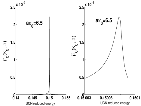
Figure 1: Coefficient $\widetilde{\mu}_{0}(k_{0},a)$ of UCN losses at $a\kappa_{0}=6.5$ against the UCN reduced energy $k_{0}^{2}/\kappa_{0}^{2}$.

UCN losses per second are determined by the integral over $k_{0}^{2}$ of the expression which is $\widetilde{\mu}_{0}(k_{0},a)$ multiplied by the magnitude of the UCN flux ${\cal F}(k_{0}^{2})$, see Sec. VI for more details. The leading contribution $\tau_{r}^{-1}$ to the integral gives the range: $w\kappa_{0}^{2}<<|k_{0}^{2}-k_{r}^{2}|<<1/a^{2}$. Since ${\cal F}(k_{0}^{2})$ is an approximately constant in the above interval, $\tau_{r}^{-1}$ is given by

$$\tau_{r}^{-1}\approx{\cal F}(k_{r}^{2})\frac{2\pi^{2}n_{0}}{\kappa_{r}k_{r}^{2}}\,w\ln[1/w(\kappa_{0}a)^{2}]\,,$$ (66)

This expression can be also derived directly from (65). Indeed, the integration of (65) over $k_{0}^{2}$ gives the result: $16\pi^{2}\Gamma_{1}\Gamma_{2}(z_{c})/(\Gamma_{2}(z_{c})+\Gamma_{1})$. This expression is integrated over $z_{c}$ by means of introducing $\Gamma_{2}(z_{c})$ as the integration variable, and eq.(66) arises.

The relation of the resonance losses to the background ones roughly is $\ln[1/w(\kappa_{0}a)^{2}]$ which is $\sim 10$ under the conditions considered. Generally, the resonance in the partial amplitude (61) increases an average nonresonance magnitude of $ImF_{l}(\kappa,a)$ over the integration interval that increases the background piece of the UCN losses. If the resonance does not occur, then the partial amplitude (61) has a zero (in the $W=0$ limit) in the integration interval. It, generally, reduces $ImF_{l}(\kappa,a)$ that decreases the losses. As a result, partial waves of the last type contribute to the losses about a percent or smaller. These rough estimations are confirmed by the numerical results of Sec. VI. An accuracy of (59) has been estimated to be about (20–30)$\%$.

It is instructive to compare (66) with the losses from the scattering of UCN by a vacuum cavity [6]. By contrast to foresaid, in the last case $U_{d}=W=0$ in (45) , but the imaginary part $U^{\prime\prime}=\eta U^{\prime}$ of the $U$ potential is taken into account. Examining (33) with $U_{d}=W=0$ and at $a\kappa\to\infty$, one concludes that the resonance piece of the UCN losses is again given by (65) with the understanding that $\Gamma_{1}$ is $\Gamma_{1}=\eta k_{r}^{2}/(a\kappa_{r})$ and, in addition, that $\Gamma_{2}(z_{c})$ and $\epsilon(z_{c})$ are calculated by (61) at $\beta=0$. For $l=0$ it agrees with the expression (17) of appendix 6.13 in [6] taking into account the difference in the definition of the average cross section and up to certain inaccuracies in [6]. Instead of (66), the UCN losses $\tau_{cv}^{-1}$ per second are now as follows:

$$\tau_{cv}^{-1}\approx{\cal F}(k_{r}^{2})\frac{2\pi^{2}n_{0}}{\kappa_{r}^{2}\kappa_{0}^{2}a}\eta\log[1/\eta(\kappa_{0}a)]\,.$$ (67)

The relation of (66 to (67) is mainly as was announced in the Introduction .

5 Possible increasing of UCN losses for non-spherical impurities

The leading contribution to the UCN losses at large $a$ is given by the sum over resonances of fractional losses (66). If the resonance is degenerated in some quantum number, then it is represented by a single term in the sum. Indeed, the numerator and the denominator in (64) each is proportional to the number of the degenerated resonances. In particular, each a resonance in the $l$-wave partial amplitude is $(2l+1)$-degenerated with respect to the azimuthal quantum number, but its contribution (64) to $\widetilde{\mu}_{0}(k_{0},a)$ contains no $(2l+1)$-multiplier. A spherical shape distortion is able to split the resonance into the $(2l+1)$ resonances. Then the UCN losses due to this resonance could increase by about $(2l+1)$ times. Nevertheless, the volume occupied by impurity could remain about the same. It is demonstrated below with an example of a small quadruple distortion of the spherical impurity when the shape of the impurity is given by

$$r=a+\frac{1}{2}\varepsilon_{ps}n_{p}n_{s},\quad\varepsilon_{ss}=0,\quad\varepsilon_{ps}=\varepsilon_{sp},n_{s}=r_{s}/r,\quad n_{s}^{2}=1,\quad\varepsilon_{rs}^{2}<<a^{2}\,,$$ (68)

where the $\varepsilon_{ps}$ set gives the shape distortion. The summation over twice-repeated indices is performed. In this case $r_{s}$ is the $s$-component of the radius-vector ${\bf r}$, and the center of the spherical impurity is placed in the point of origin. For the sake of simplicity, only mixing of states within the $l=1$ multiplet is considered. The wave vector of the falling wave is kept to be $(0,0,i\kappa)$. If $a\kappa_{0}>>1$, then the $l=1$ piece $\psi_{mat}({\bf r})$ of the UCN wave function outside the impurity, and its derivative $\psi_{mat}^{\prime}({\bf r})$ with respect to $r$, are given by

$$\psi_{mat}({\bf r})\approx-\frac{3e^{\kappa r}}{2\kappa r}n_{3}+{\bf fn}\frac{e^{-\kappa r}}{r}\,,\quad\psi_{mat}^{\prime}({\bf r})\approx-\frac{3e^{\kappa r}}{2r}n_{3}-{\bf fn}\frac{e^{-\kappa r}\kappa}{r}\,.$$ (69)

Only the exponentially large term is kept in the falling wave in (69) for the calculation of the resonance piece of the scattering amplitude ${\bf fn}$ in the leading approximation. The $l=1$ piece $\psi_{imp}({\bf r})$ of the UCN wave function inside the impurity nearby the boundary (68), and its derivative $\psi_{imp}^{\prime}({\bf r})$ with respect to $r$ are given by

$$\psi_{imp}({\bf r})\approx\frac{\cos\widetilde{k}r}{r}{\bf dn}\,,\quad\psi_{imp}^{\prime}({\bf r})\approx-\frac{\widetilde{k}\sin\widetilde{k}r}{r}{\bf dn}\,,$$ (70)

where ${\bf d}=(d_{1}\,,d_{2}\,,d_{3})$ is an independent of ${\bf r}$.

At $\varepsilon_{rs}=0$, the resonance magnitude $k_{r}$ of the wave vector is found from eq.(62) at $l=1$ (and $\alpha_{1}=0$). To find the leading term in the backward amplitude, the linear in $\varepsilon_{rs}$ terms on the boundary (68) need to be kept only in (70). Then equations matching the wave functions (69) and (70) on the impurity boundary (68), are as follows ($r=1,\,2,\,3$):

$$-\frac{3e^{\kappa a}}{2\kappa a}\delta_{r3}=\frac{e^{-\kappa a}}{a}\,f_{r}+\frac{\cos\widetilde{k}a}{a}\,d_{r}-\frac{\widetilde{k}\sin\widetilde{k}a}{5a}\varepsilon_{rs}d_{s}\,,$$

$$\frac{3e^{\kappa a}}{2a}\delta_{r3}=\frac{e^{-\kappa a}\kappa}{a}\,f_{r}+\frac{\widetilde{k}\sin\widetilde{k}a}{a}d_{r}+\frac{\widetilde{k}^{2}\cos\widetilde{k}a}{5a}\varepsilon_{rs}d_{s}\,,$$ (71)

where $\delta_{rs}$ is the Kronecker symbol, and the summation over twice-repeated indices is implied. From (71), the backward amplitude $F(\kappa,a,-1)\approx-f_{3}$ about the resonance (62) is found to be

$$F(\kappa,a,-1)\approx-\frac{12k_{r}^{2}(1+\beta)e^{2\kappa_{r}a}\det_{33}[\widetilde{x}\delta_{js}+2k_{r}^{2}\varepsilon_{js}/(5a)]}{a(\kappa_{r}^{2}+\beta k_{r}^{2})\det[(\widetilde{x}+i\,w\kappa_{0}^{2})\delta_{js}+2k_{r}^{2}\varepsilon_{js}/(5a)]}\,,\widetilde{x}=k_{0}^{2}-k_{r}^{2}\,,$$ (72)

where $\det[\widetilde{x}\delta_{js}+2k_{r}\varepsilon_{js}/5]$ is the determinant of the matrix whose elements are given in the square brackets ($j,s=1\,,2\,,3$) of the above expression, and $\det_{33}[\widehat{x}\delta_{js}+2k_{r}\varepsilon_{js}/5]$ is (33)-minor of the determinant. To obtain the coefficient of the UCN losses, the amplitude (72) is substituted into (59). One can see that (72) has the resonance, if $\widetilde{x}=x_{j}=-2k_{r}^{2}\varepsilon_{j}/(5a)$ where $\varepsilon_{j}$ is an eigenvalue of the $\{\varepsilon_{js}\}$ matrix. If $a^{2}|x_{j}-x_{s}|>>1$ for any discussed $x_{j}$ and $x_{s}$, then the UCN losses will be the sum over the losses from every resonance, they will be three time more than the UCN losses in the $\varepsilon_{rs}=0$ case. The volume $V_{im}$ occupied by impurity increases as follows:

$$V_{im}=\int d\cos\theta d\phi\,\frac{4\pi}{3}\biggl{(}a+\frac{1}{2}\varepsilon_{rs}n_{r}n_{s}\biggl{)}^{3}\approx\frac{4}{3}\pi a^{3}\biggl{(}1+\sum_{i=1}^{3}\frac{5x_{i}^{2}}{8a^{2}k_{r}^{2}}\biggl{)}\,.$$ (73)

Hence the relative change of the impurity volume goes to zero when $a\to\infty$. So, in the $a\to\infty$ limit, the distortion of the impurity shape can increase the UCN losses remaining the impurity volume being about the same. As of now, it has not been studied whether the discussed increasing of the UCN losses takes place in a realistic range of $a$.

6 Probability of UCN losses

In this Section, there is given UCN losses from ice, spherical impurities calculated under conditions where the losses have been measured experimentally. An example of a radius impurity distribution is proposed which fits the experimental losses of UCNs in the beryllium trap. As it was noted in the Introduction, now experimental data are insufficient to fit them in the unique way. The proposed fitting must be considered only as an preliminary example.

$h_{0}$	58	52	46	38	23
$\gamma(h_{0})$	0.4867	0.4608	0.4334	0.3940	0.3065
$a_{r}(1,h_{0})$	5.109	5.424	5.791	6.391	8.120
$a_{r}(2,h_{0})$	7.758	8.206	8.728	9.583	12.05

Table 1: Reduced wave vector $\gamma(h_{0})$ and $a_{r}(l,h_{0})$ impurity radius.

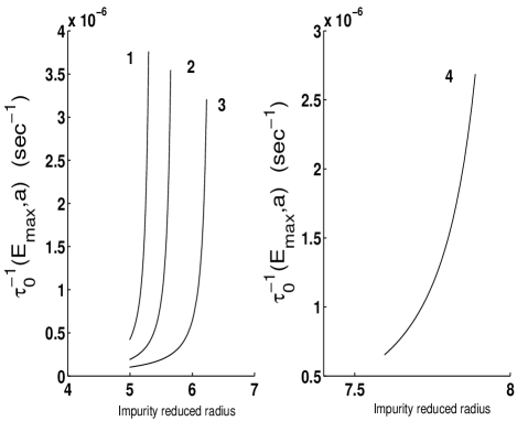
Figure 2: Probability $\tau_{0}^{-1}(E_{\rm max},a)$ of UCN losses against the impurity reduced radius in the region where resonances are not available; the trap high is 52 cm (curve 1), 46 cm (curve 2), 38 cm (curve 3) and 23 cm (curve 4).

The calculations are performed for a narrow cylindrical beryllium trap [1], its radius $R$ being $R=38$ cm, and its length $L$ being $L=14$ cm. Numerical data (52) are imployed.

For each of five discharges [1] the height $h_{0}$ of the trap is respectively 58 cm, 52 cm, 46 cm, 38 cm and 23 cm. Simultaneously, $h_{0}$ measures $E_{\rm max}$ in centimeters. The reduced wave vector $k_{max}/\kappa_{0}$ assigned to $E_{\rm max}$, will be denoted as $\gamma(h_{0})$ where $h_{0}$ is measured by centimeters. As an example, $\gamma(58)$ is the reduced wave vector assigned to $h_{0}=58$ cm. The reduced impurity radius $a\kappa_{0}$ is kept within the range $4.994\leq a\kappa_{0}\leq 9.633$ where the low limit corresponds to the $s$-resonance being at $\gamma=\gamma(58)+0.01=0.4967$, and the top limit corresponds to the $d$-resonance at $\gamma=\gamma(63)+0.01=0.5173$. An $l$-wave resonance is occurs at $E=E_{\rm max}$ at a certain reduced radius of the impurity. This reduced radius will be denoted as $a_{r}(l,h_{0})$ where $h_{0}$ is measured by centimeters. The reduced radii in the region of interest are given in Tab.1.

Experimentalists [1] determine a probability of the losses per second $\tau^{-1}(E_{\rm max})$ of UCNs with energies up to the given maximal energy $E_{\rm max}$. In line with the foregone text, it is useful to introduce in addition $\tau_{0}^{-1}(E_{\rm max},a)$, which is probability of UCN losses per second caused

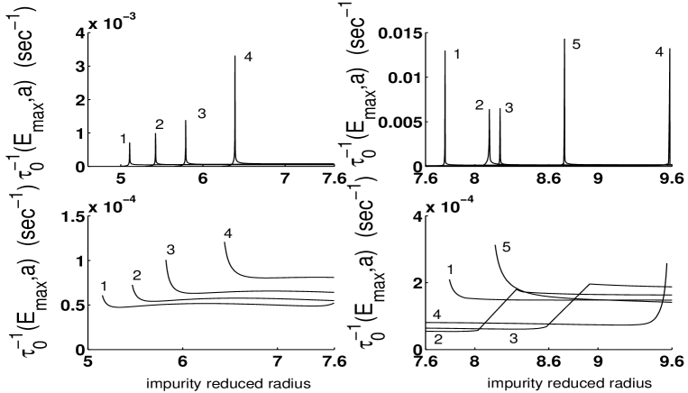
Figure 3: UCN losses $\tau_{0}^{-1}(E_{\rm max},a)$ versus the impurity reduced radius $a\kappa_{0}$ for $4.99\leq a\kappa_{0}\leq 7.6$ where only $s$-resonance is available and for $7.6\leq a\kappa_{0}\leq 9.6$ where $s$- and $p$-resonances are available; the trap height is 58 cm (curves 1), 52 cm (curves 2), 46 cm (curves 3), 38 cm (curves 4) and 23 cm (curves 5).

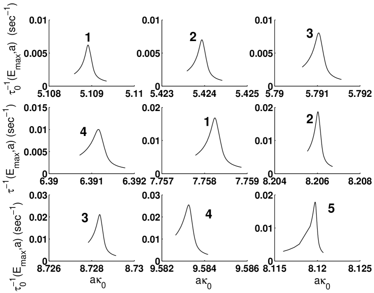
Figure 4: UCN losses $\tau_{0}^{-1}(E_{\rm max},a)$ versus $a\kappa_{0}$ in the region of the picks; the trap high is 58 cm (curves 1), 52 cm (curves 2), 46 cm (curves 3), 38 cm (curves 4) and 23 cm (curves 5).

by the UCN capture by impurities of the given radius $a$ and of the density $n_{0}=10^{14}$/cm³. Hence $\tau_{0}^{-1}(E_{\rm max},a)$ and $\tau^{-1}(E_{\rm max})$ are given by

$$\tau_{0}^{-1}(E_{\rm max},a)=\frac{1}{N_{1}(E_{\rm max})}\int\rho(k_{0},h)\frac{\hbar k_{0}}{m}\widetilde{\mu}_{0}(E,a)\,k_{0}dk_{0}\,dS\,,$$ (74)

$$\tau^{-1}(E_{\rm max})=\int_{0}^{\infty}n_{0}\frac{dn(a)}{da}\tau_{0}^{-1}(E_{\rm max},a)da\,,$$ (75)

where $\widetilde{\mu}_{0}(E,a\kappa_{0})$ is an averaged coefficient of the UCN losses (25), $n_{0}dn(a)$ is the impurity density in the $(a,a+da)$ range, and $\rho((k_{0},h)$ is the energy-space density of UCNs in the trap which will be discussed below. In this case $h$ is the height $h$ of UCN over the base of the trap The integrations in (74) are performed over the surface of the trap and over $k_{0}$ from $k_{0}=0$ to $k_{0}=k_{max}=\sqrt{2mE_{\rm max}/\hbar^{2}}$. Furthermore, $4\pi\,N_{1}(E_{\rm max})$ is the total number of UCNs in the trap as follows:

$$N_{1}(E_{\rm max})=\int\rho(k_{0},h)\,k_{0}dk_{0}\,dV\,,$$ (76)

where the integrations are performed over the volume of the trap, and over $k_{0}$ from $k_{0}=0$ to $k_{0}=k_{max}$.

$a\kappa_{0}$	5.25	5.50	5.75	6.00	6.25	6.50	6.75	7.00	7.25	7.50
s-wave only.	4.819	4.837	5.023	5.125	5.151	5.122	5.051	4.953	4.834	4.700
(s+p)-waves	4.826	4.844	5.031	5.136	5.165	5.140	5.077	4.992	4.907	4.940

Table 2: Comparison of UCN losses/sec. $\tau_{0}^{-1}(E_{\rm max},a)\times 10^{5}$ at $E_{\rm max}=58$cm due to $s$ and $(s+p)$ (the last line) interaction in the region where $p$-resonance is unavailable.

A common assumption [1, 6] is that inside the trap UCNs have the isotropic velocity distribution. Furthermore, due to the Earth gravitation field, the UCN energy is related with the height $h$ of UCN over the base of the trap as $mgh=E_{\rm max}-E$, where $g$ is the acceleration of the gravity. So the UCN density $\rho(k_{0},h)$ in both the space and the momentum space is given by a $\delta$-function type expression as follows [1, 6]:

$$\rho(k_{0},h)=c_{1}\delta(mgh-E_{\rm max}+E)\,k_{0}\,,$$ (77)

where $c_{1}$ does not depend on the UCN wave vector and on the UCN location. An explicit expression of $\tau_{0}^{-1}(E_{\rm max},a)$ for the considered trap is given in Appendix B, see eq.(B.2).

Fig.2 shows UCN losses in a region where resonances do not occur. As it has been noted already, in this case the losses are very small, $\tau_{0}^{-1}(E_{\rm max},a)\sim(10^{-6}-10^{-7})$/sec. If only a $s$-wave resonance occurs in the scattering amplitude, then solely the $s$-wave UCN-impurity interaction is important. It is demonstrated by Tab.2 at $E_{\rm max}=58$ cm where the losses due to the $s$-wave UCN-impurity interaction are compared with the losses calculated when, in addition, the $p$-wave UCN-impurity interaction is taken into account.

If a resonance is present in the UCN-impurity scattering amplitude, then UCN losses increase as it is demonstrated by Fig.3. When the resonance firstly occurs (it is an $s$-wave resonance) at $E=E_{\rm max}$, a high peak arises. Then the losses fall, but remain rather large, $\tau^{-1}(E_{\rm max})\approx(0.5$ – $1)\times 10^{-4}$/sec. The losses sharply increase again when the second resonance (it is an $p$-wave resonance) occurs. Then the losses fall, but remain to be $\approx(1$ – $2)\times 10^{-4}$/sec. In Fig.3 UCN loss probabilities are also separately presented for off peak regions (the bottom figures). Peak tops are not seen in Fig.3 because of the peaks are extremely narrow. The UCN losses within peaks are shown in Fig.4. The UCN losses are quite large in the peak ranges, but the integral contribution from the peak to the UCN losses is not prevailing because of the extremely narrow width of the peak.

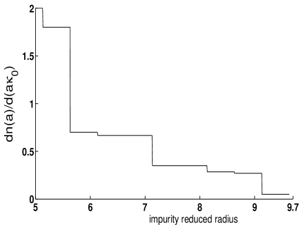
Figure 5: An example of the impurity nondimensional density $dn(a)/(da\kappa_{0})$ fitting Serebrov’s data.

Experimentally measured UCN losses [1] can be fitted, for instance, by means of the impurity piecewise-smooth radius distribution as shown in Fig.5. In this case an impurity nondimensional density $dn(a)/(da\kappa_{0})$ is given against the impurity reduced radius $a\kappa_{0}$. The impurity density in the $(a,a+da)$ range is $n_{0}\,\kappa_{0}\,da\,dn(a)/(da\kappa_{0})$. As above, $n_{0}=10^{14}$/cm³. Eqs. (74), (75) and (B.1) are employed in the calculation. In Tab.3 UCN loss probabilities $\tau^{-1}(E_{\rm max})$ calculated for the impurity radius distribution in Fig.5, are compared with the experimental data [1].

$h_{0}$	58	52	46	38	23
Serebrov’s data	21.8	17.4	15	11	8
Theor	20.7	17.9	14.2	11.4	7.9

Table 3: Serebrov’s data (the second line) compared with UCN losses under an impurity radius distribution given in Fig.5 (Theor).

The impurity density $n$ within the radius range considered is calculated as follows:

$$n=n_{0}\int_{a_{min}}^{a_{max}}\frac{dn(a)}{da}da=2.85\times 10^{14}/{\rm cm}^{3}\,,$$ (78)

where $a_{min}=4.994/\kappa_{0}$ and $a_{\rm max}=9.633/\kappa_{0}$. The average radius $a_{av}$ corresponding to Fig.5, is found to be $a_{av}=6.33/\kappa_{0}=575$ Å, and a portion $p_{V}$ of the volume occupied by impurities is $p_{V}=0.25$. As it was discussed in Sec. V, a distortion of the spherical shape impurity is potentially able to reduces $p_{V}$.

Acknowledgments

The author is grateful to A.P.Serebrov who attracts his attention to the problem of ultracold neutron losses, and for useful discussions. The author is grateful V.Yu. Petrov for collaboration and useful discussions.

This work was partial supported by RSGSS-3828.2008 grant RFFI.

Appendix Appendix A Interference effects from impurities

Effects from the interference of scattered waves are briefly discussed here. The $s$-wave USN-impurity interaction is only taken into account.

Impurities being $N$ in number, $\widetilde{\psi}_{0}({\bf r},\overrightarrow{p},\{\alpha\})$ in (6) is given by

$$\widetilde{\psi}_{0}({\bf r},\overrightarrow{p},\{\alpha\})=\sum_{i=1}^{i=N}A_{i}\frac{e^{-\kappa|{\bf r}-{\bf r_{i}}|}}{|{\bf r}-{\bf r_{i}}|}\,,$$ (A.1)

where ${\bf r_{i}}$ is the radius-vector of the i-th impurity center, and the $A_{i}$ set is calculated by the matching of the wave function off impurities with the UCN wave function inside each an impurity as follows:

$$e^{i\overrightarrow{p}\cdot\overrightarrow{l}_{n}-\widehat{\kappa}(p)z_{n}}F_{n}+F_{n}\sum_{\neq n}sA_{s}e^{-\kappa r_{ns}}/r_{ns}=A_{n}\,,n=1\,\ldots,N\,;\quad r_{nm}=|{\bf r_{n}-r_{m}}|\,,$$ (A.2)

where $F_{n}$ is the UCN scattering amplitude on the $n$-th single impurity. So the $A=\{A_{s}\}$ column is found to be

$$A=(F^{-1}-\widetilde{y})^{-1}u\,,$$ (A.3)

where $u=\{u_{n}\}$, $F=\{F_{nm}\}$ and $\widetilde{y}=\{\widetilde{y}_{nm}\}$ are given by

$$u_{n}=e^{i\overrightarrow{p}\cdot\overrightarrow{l}_{n}-\widehat{\kappa}(p)z_{n}}\,,\quad\widetilde{y}_{nn}=0,\quad F_{nm}=\delta_{nm}F_{m}\,,$$

$$\widetilde{y}_{nm}=e^{-\kappa r_{nm}}/r_{nm}\,\,\,{\rm for}\,\,n\neq m;\quad\widetilde{y}_{mm}=0\,.$$ (A.4)

Thus the effect of $n$-th and of $m$-th impurity on each other is negligible when $F_{n}\widetilde{y}_{nm}$ and $F_{m}\widetilde{y}_{nm}$ both are small. Even when $F_{n}=100$ km, $F_{n}\widetilde{y}_{nm}$ is less than $0.01$ already for $|\overrightarrow{l_{n}-l_{m}}|=1.5\times 10^{-5}$ cm. The macroscopic effect is due to the interference from those scatterers, which separated from each other by a macroscopic scale distances being much more than the distance above. So $A_{n}$ can be approximated by the relevant amplitude of the UCN scattering on the single isolated impurity.

To discuss the interference under the reflection of the UCN from the trap boundary, one notes that in the discussed case, $\widetilde{B}(\overrightarrow{q,k_{0}},\{\alpha\})$ is found from eq.(15) with the understanding that now the function $\widetilde{\psi}_{0}({\bf r},\overrightarrow{p},\{\alpha\})$ is given by (A.1). In this case $\widetilde{B}(\overrightarrow{q,k_{0}},\{\alpha\})$ is found to be

$$\widetilde{B}(\overrightarrow{q,k_{0}},\{\alpha\})=\sum_{s=1}^{N}\sum_{s^{\prime}=1}^{N}\frac{\widehat{k}_{0}(q_{0})e^{-i\overrightarrow{q}\cdot\overrightarrow{l_{s}}}e^{-\widehat{k}(q)z_{s}}e^{i\overrightarrow{q_{0}}\cdot\overrightarrow{l_{s^{\prime}}}}e^{-\widehat{k}(q_{0})z_{s^{\prime}}}}{\pi\widehat{\kappa}(q)(\widehat{k}_{0}(q_{0})+i\widehat{\kappa}(q_{0}))}B_{ss^{\prime}}\,,$$ (A.5)

where $B_{ss^{\prime}}=B_{s^{\prime}s}$ and the matrix $B=\{B_{ss^{\prime}}\}$ satisfies an equation as follows:

$$B=(F^{-1}-\widehat{x})^{-1}[1-(J^{(d)}+\widehat{J})B]\,.$$ (A.6)

Hence $B$ is found to be

$$B=(F^{-1}-\widehat{x}-J^{(d)}-\widehat{J})^{-1}\,,$$ (A.7)

where matrix elements of matrices $\widehat{J}=\{\widehat{J}_{mn}\}$ and $J^{(d)}=\{J_{mn}^{(d)}\}$ are given by

$$\widehat{J}_{nm}=\widehat{J}_{mn}=\int e^{i\overrightarrow{q}\cdot(\overrightarrow{l_{n}}-\overrightarrow{l_{m}})}\,\frac{e^{-\widehat{\kappa}(q)(z_{n}+z_{m})}\,[\widehat{k}_{0}(q)-i\widehat{\kappa}(q)]}{\widehat{\kappa}(q)[\widehat{k}_{0}(q)+i\widehat{\kappa}(q)]}\frac{d^{2}q}{2\pi}\,,\quad J^{(d)}_{sn}=-\delta_{sn}\widetilde{C}_{00}^{(0)}(z_{n},\kappa)\,,$$ (A.8)

where $\widehat{C}_{00}^{(0)}(z_{n},\kappa)$ is given by (43). Due to a singularity at $q^{2}=k_{0}^{2}$ in the integrand, $\widehat{J}_{mn}$ decreases at $|\overrightarrow{l_{n}}-\overrightarrow{l_{m}}|\to\infty$, as follows:

$$\widehat{J}_{mn}\to 2(1+i)k_{0}e^{-\kappa_{0}(z_{m}+z_{n})}\frac{e^{k_{0}|\overrightarrow{l_{n}}-\overrightarrow{l_{m}}|}}{\kappa_{0}^{2}|\overrightarrow{l_{n}}-\overrightarrow{l_{m}}|^{2}}\,,$$ (A.9)

that is nonexponentially. To obtain (A.9) one first integrates in $\widehat{J}_{mn}$ over the azimuth angle $\phi$, keeping $|\overrightarrow{l_{n}}-\overrightarrow{l_{m}}|\to\infty$. The obtained integral is represented as

$$\widehat{J}_{mn}\approx 2\int_{k_{0}}^{\infty}e^{iq|\overrightarrow{l_{n}}-\overrightarrow{l_{m}}|}\frac{e^{-\widehat{\kappa}(q)(z_{n}+z_{m})}\,[\widehat{k}_{0}(q)-i\widehat{\kappa}(q)]}{\widehat{\kappa}(q)[\widehat{k}_{0}(q)+i\widehat{\kappa}(q)]}\sqrt{\frac{q}{2\pi}}dq+\int_{-\infty+0}^{\infty+0}\ldots\,dq\,,$$ (A.10)

where ellipses denote the integrand in the last integral. The above integrand is the same as in the first term. The last integral decreases exponentially when $|\overrightarrow{l_{n}}-\overrightarrow{l_{m}}|\to\infty$. The calculation of the first integral leads to (A.10).

By using (18), (23) and (A.5), the averaged cross section $\widetilde{\sigma}_{c}(k_{0},\{\alpha\})$ of the UCN losses in the $\widetilde{y}=0$ approximation is found to be

$$\widetilde{\sigma}_{c}(k_{0},\{\alpha\})=-\frac{4\pi}{k_{0}^{2}}\sum_{m,n=1}^{N}(ImJ^{(d)}+Im\widehat{J})_{mn}\,|F^{-1}-J^{(d)}-\widehat{J}|^{-1}_{mn}ImF^{-1}_{n}\prod_{s=1}^{N}\frac{d^{2}l_{s}}{S}\,,$$ (A.11)

where an averaging over each $\overrightarrow{l}_{s}$ is performed, as well. Thus the $\Delta$ correction in $\widetilde{\sigma}_{c}(k_{0},\{\alpha\})$ due to the two impurity interference is as follows:

$$\Delta=-\frac{4\pi}{k_{0}^{2}}\sum_{m,n=1}^{N}\frac{ImJ^{(d)}_{m}\,ImF^{-1}_{n}|\widetilde{J}_{mn}|^{2}+Im\widetilde{J}_{mn}\,ImF^{-1}_{n}\,2Re[\widetilde{J}_{mn}(F^{-1}_{n}-J^{(d)}_{n})}{\biggl{|}(F_{m}^{-1}-J^{(d)}_{m})(F_{n}^{-1}-J^{(d)}_{n})\biggl{|}^{2}}\prod_{s=1}^{N}\frac{d^{2}l_{s}}{S}\,.$$ (A.12)

From (A.9), a relative correction (A.12) to the leading term of $\widetilde{\sigma}_{c}(k_{0},\{\alpha\})$ is roughly found to be $\sim N/(S\kappa_{0}^{2})\sim n\,d_{0}/\kappa_{0}^{2}$, where $d_{0}$ is the length of the trap coating, $d_{0}\approx 5000$ Å, and $n$ is the impurity density. This correction is extremely small for any reasonable $n$.

So, (A.11) is a sum of the losses over the UCN losses from each a single, isolated impurity, as it is considered throughout this paper.

Appendix Appendix B UCN losses in a cylindrical trap

To obtain $\tau_{0}^{-1}(E_{\rm max},a)$ in the case of interest, cylindrical coordinates $(\rho,\phi,z)$ are employed. In this case $z$-axis goes along the length of the cylinder laying horizontally, $\rho$ is a minimal distance from the given space point to $z$-axis, and $\psi$ is an angle in the perpendicular to $z$-axis plane, $\psi=0$ at the bottommost point of the trap. The infinitesimal element $dS$ of the side surface is $dS=Rdzd\psi$, and for each of the butt-end, $dS=\rho\,d\rho\,d\psi$. The integration over $\psi$ is performed employing $\delta$-function in (77). The integration with respect to $z$ over the side and with respect to $\rho$ over the butt-ends are performed without difficulties. Then (77) is found to be

$$\tau_{0}^{-1}(E_{\rm max},a)=\frac{2U}{\hbar N(h_{0})L\kappa_{0}}\int\frac{k_{0}^{2}}{\kappa_{0}^{2}}\widetilde{\mu}_{0}(E,a)\Biggl{[}\frac{2RL}{L_{0}^{2}\sqrt{R^{2}/L_{0}^{2}-[k_{0}^{2}/\kappa_{0}^{2}-h_{0}/L_{0}+R/L_{0}]^{2}}}$$

$$+4\sqrt{R^{2}/L_{0}^{2}-[k_{0}^{2}/\kappa_{0}^{2}-h_{0}/L_{0}+R/L_{0}]^{2}}\Biggl{]}\frac{dk_{0}^{2}}{\kappa_{0}^{2}}\,,$$ (B.1)

where

$$L_{0}=U/mg\,,\qquad h_{0}=E_{\rm max}/mg\,.$$ (B.2)

In the calculation of $N_{1}(e_{\rm max})$ one integrates over $E$ employing the $\delta$-function in (77) and integrates over $z$. In doing so $dV=\rho d\rho\psi dz$. The result is as it follows:

$$N(h_{0})=\int\frac{\rho\,d\rho}{L_{0}^{2}}\,d\psi\sqrt{(\frac{\rho}{L_{0}}\cos\psi-\frac{R}{L_{0}}\cos\psi_{0})}\,,$$ (B.3)

where

$$R-R\cos\psi_{0}=h_{0}\,.$$ (B.4)

The integration in (B.3) is performed keeping the radicant being positive and in addition, $\psi<\psi_{0}$ and $\rho<R$. The integral can be calculated through Legendre function $P_{1/2}^{-2}(1-h_{0}/R)$ as follows:

$$N(h_{0})=\biggl{(}\frac{R}{L_{0}}\biggl{)}^{5/2}\frac{\pi}{\sqrt{2}}\biggl{[}1-\biggl{(}1-\frac{h_{0}}{R}\biggl{)}^{2}\biggl{]}P_{1/2}^{-2}(1-h_{0}/R)\,.$$ (B.5)

Below eq.(B.5) is proved for $\psi_{0}<0$. The calculation for $\psi_{0}>0$ is performed in the same manner.

For $\psi_{0}<0$, there are two integration regions in $\psi$ and $\rho$ being as follows:

$$0<|\psi|<|\psi_{0}|\,,\quad 0<\rho<R\quad({\rm region1})\quad{\rm and}$$

$$|\psi_{0}|<|\psi|<\pi\,,\quad 0<\rho|\cos\psi|<R|\cos\psi_{0}|\,\,({\rm reg.2}).$$ (B.6)

The integral over each a region will be denoted respectively as $\widetilde{N}_{1}(h_{0})/L_{0}^{5/2}$ and $N_{2}(h_{0})/L_{0}^{5/2}$. The integration over $\rho$ is performed using that the indefinite integral

$$I=\int\rho\,d\rho\sqrt{(\rho\cos\psi-R\cos\psi_{0})}$$ (B.7)

is equal to

$$I=\frac{2\rho}{3\cos\psi}(\rho\cos\psi-R\cos\psi_{0})^{3/2}-\frac{4}{15\cos^{2}\psi}(\rho\cos\psi-R\cos\psi_{0})^{5/2}\,.$$ (B.8)

Hence

$$\widetilde{N}_{1}(h_{0})=\int\,d\psi\Biggl{[}\frac{2R^{5/2}}{3\cos\psi}(\cos\psi-\cos\psi_{0})^{3/2}-\frac{4R^{5/2}}{15\cos^{2}\psi}\biggl{[}(\cos\psi-\cos\psi_{0})^{5/2}-(-\cos\psi_{0})^{5/2}\biggl{]}\Biggl{]}\,,$$ (B.9)

and

$$\widetilde{N}_{2}(h_{0})=4\int\,d\psi\frac{4R^{5/2}}{15\cos^{2}\psi}(-\cos\psi_{0})^{5/2}\,.$$ (B.10)

The second term in (B.9) is integrated by part using that $d\psi/\cos^{2}\psi=d\tan\psi$. Hence

$$\widetilde{N}_{1}(h_{0})=\frac{2R^{5/2}}{3}\int\,d\psi\,\cos\psi(\cos\psi-\cos\psi_{0})^{3/2}-\frac{8R^{5/2}}{15}\sin\psi_{0}(-\cos\psi_{0})^{3/2}\,.$$ (B.11)

Furthermore,

$$\frac{2R^{5/2}}{3}\int\,d\psi\,\cos\psi(\cos\psi-\cos\psi_{0})^{3/2}=\pi\frac{R^{5/2}}{\sqrt{2}}\sin^{2}\psi_{0}P^{-2}_{1/2}(\cos\psi_{0})\,,$$ (B.12)

where $P^{-2}_{1/2}$ is the Legendre function. The $\widetilde{N}_{2}(h_{0})$ integral is easy calculated, and as a final result, (B.5) arises.

References

[1]
A. P. Serebrov, Uspehi Fiz. Nauk 175, 905 (2005)
[Physics-Uspekhi 48, 885 (2005)];
A. Serebrov, N. Romanenko, O. Zherebtsov, M.
Lasakov, A. Vasilyev, A. Fomin, P. Geltenbort I. Krasnoshekova, A.
Kharitonov and V. Varlamov, Phys. Lett. A 335, 327 (2005);
[2]
V. P. Alfimenkov,
V. V. Nesvizhevky, A. P. Serebrov, A.V. Strelkov, R. R. Talidaeva, A.
G. Kharitonov and V. N. Shvetsov, Pis’ma Zh. Eksp. Teor. Fiz. 55, 92 (1992) [JETP Letters 55, 84 (1992) ].
[3]
S. S. Arzumanov, L. N.
Bondarenko, V. I. Morozov, Yu. N. Panin and P. Geltenbort, Yad. Fiz.
66,1868 (2003) [Phys. Atom. Nucl. 66, 1820
(2003)].
[4]
L. N. Bondarenko, P. Geltenbort, E. I. Korobkina, V. I. Morozov and Yu.
N. Panin, Yad. Fiz. 65, 13 (2002) [Phys. At. Nuclei
65, 11 (2002)]; A. P. Serebrov et al., Phys. Lett A
309, 218 (2003); A. Steyerl, B. G. Yerozolimsky, A.P.
Serebrov, P. Geltenbort, N. Achiwa, Yu. N. Pokotilovski, O. Kwon, M. S.
Lasakov, I. A. Krasnoshchokina and A. V. Vasilyev, Eur. Phys. J. B
28, 299 (2002);
Yu. A. Pokotilovski, Zh. Eksp. Theor. Fiz.
123, 203 (2003) [JETP, 96, 172 (2003)].
[5]
V. V. Nesvizhvsky, Phys. Atom. Nucl.
65, 400 (2002); V. Gudkov, Nucl. Instrum. Methods, A
580, 1390 (2007);
[6]
V. K. Ignatovich, The Physics of Ultracold
Neutrons (Oxford: Clarendon Press,1990).
[7]
A. P.
Serebrov et al., Nuc. Inst. Methods, A 440, 717
(2000); Phys. Lett. A 313, 373 (2003).
[8]
A.L. Barabanov and K.V. Protasov, Phys. Lett. A 346, 378
(2005);
[9] L. D. Landau, E. M. Lifshitz, Quantum
Mechanics, 3rd ed (Permagon, Oxford. 1977)