Nonlinear inertia-gravity wave-mode interactions in three dimensional rotating stratified flows

Abstract

We investigate the nonlinear dynamics of inertia-gravity (IG) wave modes in three-dimensional (3D) rotating stratified fluids. Starting from the rotating Boussinesq equations, we derive a reduced partial differential equation, the GGG model, consisting of only wave-mode interactions. We note that this subsystem conserves energy and is not restricted to resonant wave-mode interactions. In principle, comparing this model to the full rotating Boussinesq system allows us to gauge the importance of wave-vortical-wave vs. wave-wave-wave interactions in determining the transfer and distribution of wave-mode energy. As in many atmosphere-ocean phenomena we work in a skewed aspect ratio domain $H/L$ ($H$ and $L$ are the vertical and horizontal lengths) with $Fr=Ro<1$ such that $Bu=1$, where $Fr$, $Ro$ and $Bu$ are the Froude, Rossby and Burger numbers, respectively. Our focus is on the equilibration of wave-mode energy and its spectral scaling under the influence of random large-scale ($k_{f}$) forcing. We present results from two sets of parameters: (i) $Fr=Ro\approx 0.05$, $H/L=1/5$, and (ii) $Fr=Ro\approx 0.1$, $H/L=1/3$. As anticipated from prior work, when forcing is applied to all modes with equal weight, with $Fr=Ro\approx 0.05$ and $H/L=1/5$, the wave-mode energy of the full system equilibrates and its spectrum scales as a power-law that lies between $k^{-1}$ and $k^{-5/3}$ for $k_{f}<k<k_{d}$, where $k_{d}$ is the dissipation scale. For the same parameters, when forcing is restricted to only wave modes, the wave-mode energy fails to equilibrate in both the full system as well as the GGG subsystem at the resolutions we can achieve. This cleary demonstrates the importance of the vortical mode (by facilitating wave-vortical-wave interactions) in determining the wave-mode energy in the rotating Boussinesq system. Proceeding to the second set of simulations, i.e. for the larger $Fr=Ro\approx 0.1$ in a less skewed aspect ratio domain with $H/L=1/3$, we observe that the energy of the GGG subsystem equilibrates and is resolution independent. Further, the full system with forcing restricted to wave modes also equilbrates and both yield identical energy spectra. Thus it is clear that the wave-wave-wave interactions play a role in the overall dynamics at moderate $Ro$, $Fr$ and aspect ratios. Apart from theoretical concerns addressed in the Conclusion, from a practical standpoint these results highlight the difficulty in properly resolving wave-mode interactions when simulating realistic geophysical phenomena.

I Introduction

Inertia gravity (IG) waves, resulting from the rotating and stratified nature of geophysical fluids, play an important role in atmosphere-ocean dynamics Gill . A broad overview of their properties with relevance to the ocean can be found in Garrett & Munk Garrett-Munk , and a recent review focussing on the observational characterization of the oceanic wave-field can be found in Polzin and Lvov PL . The general dynamics of these waves are reviewed by Sommeria & Staquet S-rev . Further, Wunsch & Ferrari Wunsch-Ferrari place these waves in context when considering the general circulation of the ocean, while Fritts & Alexander Fritts-Alexander review their influence on diverse phenomena in the middle atmosphere.

In their influential papers, Garrett & Munk Garrett-Munk ,GM1 pointed out the importance of a deeper understanding of the dynamics of the IG wave modes. In this regard, one avenue of progress has been to focus upon the subset of resonant interactions among these waves Mc-B . In general, the dispersive nature of the linear waves results in reduced nonlinear transfer between modes by dispersive phase scrambling. However, resonant interactions are special nonlinear interactions for which phase scrambling is absent, and nonlinear transfer remains strong. Thus resonant interactions are critical for the dynamics when they are present. See for example Anile for a broad introduction to nonlinear dispersive equations, Zak for statistical theories of the so-called weak turbulence, Majda-book , Chemin-book for geophysical perspectives and Bartello ,SS-gafd for the roles of resonances and near-resonances in the specific case of the 3D rotating Boussinesq system.

Investigating resonant IG waves, McComas & Bretherton Mc-B distinguished between three classes of resonant interactions that lead to induced diffusion, elastic scattering and parametric sub-harmonic instability. The picture put forth was, for a large-scale initial data: (i) elastic scattering leads to 3D isotropy of an initial condition that is only horizontally isotropic, (ii) sub-harmonic instability moves energy downscale, (iii) induced diffusion tends to force the high wavenumber spectrum towards equilibrium. A detailed account of these resonances can be found in the extensive review by Muller et al. Muller-rev ; their review also describes approaches that account for more than resonant interactions, but involve other approximations (such as the direct interaction approximation). Further, the use of resonances to derive kinetic equations under the weak turbulence paradigm has been an active area of work — for an overview see Lvov et al. L-web . In particular recent work has shown a correspondence between observed IG energy spectra and particular steady state solutions of the relevant kinetic equations L1 ,L2 .

Unfortunately, as was pointed out by McComas & Bretherton Mc-B , resonances do not account for the bulk of interactions among IG waves. A formal statement regarding the sparsity of these resonances can be found in Babin et al. Babin-rev . This is all the more an important issue when $Ro,Fr$ are small (implying strong rotation and stratification) but far from zero, i.e. $0\ll Ro,Fr<1$ (where $Ro,Fr$ are the Rossby and Froude numbers respectively). Indeed, having non-zero $Fr$ and/or $Ro$ opens the door for near-resonances to enter the dynamics and these interactions can, both quantitatively and qualitatively, change the behavior of the system SS-gafd . This naturally motivates the construction of a model (called the GGG model) that includes all possible wave-mode interactions. Quite interestingly, as the two-dimensional (2D) stratified Boussinesq system only supports wave modes, this new 3D system can be looked upon as an extension of the full 2D stratified problem BS ,SS ,Smith-short .

So far, our discussion has been restricted to considering wave modes in isolation. In reality rotating and stratified fluids support an additional vortical mode of motion LR , and in fact in geophysically relevant limits, interactions among vortical modes lead to the celebrated quasigeostrophic (QG) equations Bartello ,Babin-rev ,SW . Indeed, one of the many contributions by Prof. Majda (in collaboration with Prof. P. Embid) in the field of geophysical fluid dynamics concerns a formal statement on the emergence of QG dynamics, from the governing rotating Boussinesq equations, in the limit $Ro\sim Fr=\epsilon\rightarrow 0$ while holding $Bu\sim 1$ Embid1998 ,Babin-rev . In addition to clarifying the nature of the QG equations and constructing a general framework for averaging over fast-modes in geophysical systems Embid1996 , their work also predicted the emergence of a new regime, the so-called vertically sheared horizontal flows (VSHF) when $Ro\sim 1$ while $Fr=\epsilon\rightarrow 0$ Embid1998 ,MajdaEmbid . Since then, numerical work in the appropriate parameter regime has confirmed the emergence of VSHF modes when considering a rotating Boussinesq fluid under random forcing SW ,Laval ,WB1 ,WB2 .

As it happens, the vortical mode plays an important role in the redistribution of wave-mode energy by means of the so-called wave-vortical-wave interactions. In fact, this is thought to be the primary manner in which energy is transferred from large to small scales in rotating and stratified flows, and is attributed to be the fundamental mechanism behind geostrophic adjustment Bartello . Further, in both decaying and forced scenarios, numerical simulations of rapidly rotating and strongly stratified (i.e. small $Ro,Fr$) flows have shown the equilibration of wave modes (by means of the aforementioned forward transfer) while energy continues to be transferred upscale in the vortical modes via vortical-vortical-vortical (QG) interactions Bartello ,SS-gafd . For $f=N$ (where $f,N$ are the Coriolis parameter and the Brunt-Väisälä frequency) in a unit aspect ratio, the wave modes are passively driven by the vortical modes. For this case $f=N$, there are no wave-wave-wave resonances (or near-resonances), and the distribution of energy among the wave modes is strongly influenced by the presence of the vortical mode Bartello ,SS-gafd . Of course, in the atmosphere-ocean system $f\neq N$, leading to the possibility of near and exact wave-wave-wave resonances, though as stated earlier these sets of interactions are sparse Babin-rev . All in all, this line of reasoning leads one to believe that the vortical mode should in fact play a significant role in determining the wave-mode energy distribution.

These scenarios then lead to a somewhat dichotomous state of affairs with regard to IG wave-mode energy, i.e. on one hand we have theories based on the interactions of IG modes in isolation. On the other hand, there is reason to attribute a prominent role to the vortical mode in the overall dynamics of a rotating and stratified fluid, which includes the distribution of energy among the wave modes themselves. This dichotomy — in the context of purely stratified flows — has been pointed out and investigated by Waite & Bartello WB2 . By forcing only wave modes of the Boussinesq system, they inquired into the turbulence generated by a stratified fluid. Their principal conclusion was to highlight the importance of the vortical mode in mediating wave-mode energy transfer and distribution. Further, they noted the difficulty in properly resolving wave-mode interactions WB2 . In the present work, in addition to studying the full Boussinesq equations, we derive a model that consists of only wave-mode interactions, which in principle provides the means for determining the relative importance of wave-vortical-wave and wave-wave-wave interactions for the distribution of wave-mode energy. Specifically, by simulating the newly derived GGG model, we attempt to see if this system is capable of a robust forward transfer of energy, and compare the energy spectra of wave modes from the GGG model to the corresponding wave mode spectra that arise from simulations of the full rotating-stratified Boussinesq system. We proceed to introduce the basic equations, review the possible means of wave mode evolution and derive the GGG model. We then describe the numerical setup and proceed to the simulations of this system. Finally, we collect and discuss the results.

II Basic Equations

The rotating Boussinesq equations in a 3D periodic setting are Majda-book

$$\frac{{\rm D}{\bf u}}{{\rm D}t}+f\hat{z}\times{\bf u}=-\nabla\varphi-N\theta\hat{z}+\nu\nabla^{2}{\bf u}$$

$$\frac{{\rm D}\theta}{{\rm D}t}-Nw=\kappa\nabla^{2}\theta~{},~{}\nabla\cdot\mathbf{u}=0$$ (1)

where ${\bf u}=(u,v,w)$ is the 3D velocity field, $\varphi=p/\rho_{0}$ is a scaled pressure and $f$ is the Coriolis parameter with rotation assumed to be aligned with the $z$-axis. Equations (1) result from considering periodic perturbations to a state of hydrostatic balance wherein the density profile satisfies $\rho=\rho_{0}-bz+\rho^{\prime}$ with $|\rho^{\prime}|,|bz|\ll\rho_{o}$. Further, we have set $\rho^{\prime}=(N\rho_{o}/g)\theta$ where $N=(gb/\rho_{0})^{1/2}$. Finally, $\nu$ and $\kappa$ are the viscosity and diffusivity respectively.

Linearizing (1) about a state of rest, substituting solutions of the form $\phi=\hat{\phi}\exp\{{\rm i}{\bf k}\cdot{\bf x}-\sigma({\bf k})t\}$ one finds

$$\sigma_{\pm}({\bf k})=\pm\frac{(N^{2}k_{h}^{2}+f^{2}k_{z}^{2})^{1/2}}{k}~{};~{}\sigma_{0}({\bf k})=0.$$ (2)

Here $k$ is the magnitude of the wave-vector and $k_{h}^{2}=k_{x}^{2}+k_{y}^{2}$. Modes corresponding to $\sigma_{\pm}$ are the IG waves (referred to as wave modes), while the mode corresponding to $\sigma_{0}$ is referred to as the vortical (or geostrophic) mode LR ,Bartello ,SW . Denoting the eigenfunctions corresponding to $\sigma_{0},\sigma_{\pm}$ by $\phi_{0},\phi_{\pm}$ respectively, it is known that these eigenfunctions are mutually orthogonal and form a complete basis (see Embid & Majda Embid1996 , Embid1998 and Smith & Waleffe SW for details). This enables us to project a Fourier expansion of the solution to (1) onto this eigenfunction basis, i.e. projections of the form

$$\mathbf{v}({\bf k},t)=a_{0}({\bf k},t)\phi_{o}({\bf k})+a_{+}({\bf k},t)\phi_{+}({\bf k})+a_{-}({\bf k},t)\phi_{-}({\bf k}),$$ (3)

where $\mathbf{v}$ is the state vector, $\mathbf{v}^{T}=(u,v,w,\theta)$ Embid1998 , Bartello , SW . Symbolically this yields

$$\frac{\partial a_{\alpha}(\mathbf{k},t)}{\partial t}+{\rm i}\sigma_{\alpha}(\mathbf{k})a_{\alpha}(\mathbf{k},t)=\sum_{\triangle}\sum_{\beta,\gamma}C_{\mathbf{k}\mathbf{p}\mathbf{q}}^{\alpha\beta\gamma}a_{\beta}(\mathbf{p},t)a_{\gamma}(\mathbf{q},t)$$ (4)

where $\triangle$ represents a sum over ${\bf p},{\bf q}$ such that ${\bf k}={\bf p}+{\bf q}$. The indices $\alpha,\beta,\gamma$ run over $0,+,-$ and $C_{{\bf k}{\bf p}{\bf q}}^{\alpha\beta\gamma}$ is the interaction coefficient. The exact form of the interaction coefficients is not emphasized here, but it is helpful in our discussion to think in terms of the following symmetric definition

$$C_{{\bf k}{\bf p}{\bf q}}^{\alpha\beta\gamma}=\frac{-{\rm i}}{2}\left((\phi_{\beta}^{\mathbf{u}}(\mathbf{p})\cdot\mathbf{q})\phi_{\gamma}(\mathbf{q})+(\phi_{\gamma}^{\mathbf{u}}(\mathbf{q})\cdot\mathbf{p})\phi_{\beta}(\mathbf{p})\right)\cdot\phi_{\alpha}^{*}(\mathbf{k}),$$ (5)

where $\phi_{\beta}^{\mathbf{u}}$ contains the first three components of $\phi_{\beta}$ corresponding to the velocity entries and $(\cdot)^{*}$ denotes complex-conjugate. Notice that, with this symmetric definition, $C_{{\bf k}{\bf p}{\bf q}}^{\alpha\beta\gamma}=C_{{\bf k}{\bf q}{\bf p}}^{\alpha\gamma\beta}$; the coefficient $C_{{\bf k}{\bf p}{\bf q}}^{\alpha\beta\gamma}$ involves the advection of the mode corresponding to $q$ by the mode corresponding to $p$ and vice versa. In the following, a triplet $(\cdot,\cdot,\cdot)$ refers to a particular type of triad interaction, and a $v$ refers to a vortical mode while a $w$ refers to a wave mode (either a $+$ or a $-$ mode). For example, $(w,w,v)$ (with all permutations implied) represents all possible interactions between two wave modes and one vortical mode.

II.1 Wave-mode evolution

An alternate way to represent the expansion is $\mathbf{v}({\bf k},t)=b_{0}({\bf k},t)\phi_{o}({\bf k})\exp[-{\rm i}\sigma_{0}(\mathbf{k})t]+b_{+}({\bf k},t)\phi_{+}({\bf k})\exp[-{\rm i}\sigma_{+}(\mathbf{k})t]+b_{-}({\bf k},t)\phi_{-}({\bf k})\exp[-{\rm i}\sigma_{-}(\mathbf{k})t]$. In this case (4) takes the form

$$\frac{\partial b_{\alpha}(\mathbf{k},t)}{\partial t}=\sum_{\triangle}\sum_{\beta,\gamma}C_{\mathbf{k}\mathbf{p}\mathbf{q}}^{\alpha\beta\gamma}b_{\beta}(\mathbf{p},t)b_{\gamma}(\mathbf{q},t)\exp\{{\rm i}[\sigma({\bf k})-\sigma({\bf p})-\sigma({\bf q})]~{}t\}$$ (6)

which shows the influence of the dispersion on the advective nonlinearity. Indeed, it is now possible to construct a dynamical hierarchy consisting of (i) resonances, i.e. $|\sigma({\bf k})-\sigma({\bf p})-\sigma({\bf q})|=0$, (ii) near-resonances, i.e. $0<|\sigma({\bf k})-\sigma({\bf p})-\sigma({\bf q})|\leq\delta$ where $\delta=\min{(Ro,Fr)}$ and (iii) non-resonant interactions, i.e. $|\sigma({\bf k})-\sigma({\bf p})-\sigma({\bf q})|>\delta$. In this hierarchy it is postulated that resonances are always important, near-resonances play a role when $0<\delta<1$ i.e. rotation and stratification are strong, but we are outside limiting scenarios where $\delta\rightarrow 0$. Finally, for rapid rotation and strong stratification, non-resonant interactions are only expected to contribute at higher-orders (in $\delta$). While it is not possible for non-resonant interactions to lead to qualitatively different behavior as compared to near-resonances, we note that near-resonances open up pathways that are precluded under resonance (for details see Sukhatme & Smith SS-gafd ). An explicit example of such a qualitative change induced by near-resonant interactions is provided via cyclonic-anticyclonic asymmetry in rotating flows Smith-Lee . Other examples, such as the influence on the statistical features of water waves and capillary wave generation may be found in Annenkov & Shrira AnSh , and Watson & Buschbaum WaBu , respectively.

Considering only resonant and near-resonant interactions, the wave modes can only evolve via the $(w,w,v)$ and $(w,w,w)$ classes (see Bartello Bartello or Sukhatme & Smith SS-gafd for a detailed view of wave and vortical mode evolution). When $1/2\leq f/N\leq 2$ the $(w,w,w)$ (near) resonant interactions are absent and — within this dynamical hierarchy — the distribution of wave-mode energy is determined by $(w,w,v)$, indicating the crucial role played by the vortical mode. Further, it was shown by Bartello Bartello , that purely resonant $(w,w,v)$ interactions are catalytic in that they involve the exchange of energy among two wave modes by using the vortical mode as a catalyst. This leads to the elegant result that when $f=N$ the wave modes are passively driven by the vortical mode Bartello (this follows as near-resonances are not possible for a rapidly rotating and strongly stratified fluid when $f=N$ SS-gafd ). Of course, in the most general case we lift the restriction $1/2\leq f/N\leq 2$. As both $(w,w,v)$ and $(w,w,w)$ are viable means of affecting the wave-mode energy distribution, it is natural to inquire into their nature and importance. Specifically, given the formal sparsity of $(w,w,w)$ interactions Babin-rev , are $(w,w,v)$ always dominant? Indeed, do the $(w,w,w)$ interactions play any role in the 3D rotating Boussinesq system? Also, what is the nature of these interactions, i.e. do they yield a forward transfer of energy under large-scale forcing? If so, do they lead to an equilibration of wave modes and yield a well-defined power spectrum? To inquire into these questions, we construct a model (the GGG model) that includes only wave-mode interactions. In principle, comparing the results from the GGG model with the full rotating Boussinesq system should help in settling some of these issues.

II.2 The GGG model

We now present the GGG model in physical space and its derivation. It is useful to first determine the mode amplitudes in terms of the physical variables. Towards this goal, begin by defining the stream function $\psi$, the potential function $\chi$, and the horizontally averaged flows $\overline{u(z)}$ and $\overline{v(z)}$ in the standard way

$$u=\chi_{x}-\psi_{y}+\overline{u(z)}\quad\text{and}\quad v=\chi_{y}+\psi_{y}+\overline{v(z)}.$$ (7)

Here $\overline{(\cdot)}$ denotes a horizontal average. These definitions imply $\nabla_{h}^{2}\chi=u_{x}+v_{y}$ and $\nabla_{h}^{2}\psi=v_{x}-u_{y}$. Substituting (7) for $u$ and $v$ in the state vector ,$\mathbf{v}$, (3) and the orthonormality of the eigenfunctions yields (please see the Appendix for additonal details)

$$a_{k}^{0}=\frac{{\rm i}N}{\sigma_{k}k}(-k_{h}^{2}\psi-{\rm i}\frac{f}{N}k_{z}\theta)$$ (8)

$$a_{k}^{+}=\frac{1}{\sqrt{2}\sigma_{k}k}(-\frac{\sigma_{k}w_{k}k^{2}}{k_{h}}-fk_{z}k_{h}\psi+{\rm i}Nk_{h}\theta)$$ (9)

$$a_{k}^{-}=\frac{1}{\sqrt{2}\sigma_{k}k}(-\frac{\sigma_{k}w_{k}k^{2}}{k_{h}}+fk_{z}k_{h}\psi-{\rm i}Nk_{h}\theta)$$ (10)

$$a_{k_{z}}^{0}=\overline{\theta(z)}\text{sgn}(fk_{z})\quad a_{k_{z}}^{+}=\frac{-{\rm i}\overline{u}+\overline{v}}{\sqrt{2}}\quad a_{k_{z}}^{-}=\frac{{\rm i}\overline{u}+\overline{v}}{\sqrt{2}}.$$ (11)

Next, notice that by adding $a_{k}^{+}$ and $a_{k}^{-}$ and also subtracting $a_{k}^{-}$ from $a_{k}^{+}$ the physical variables decouple further,

$$a_{k}^{+}+a_{k}^{-}=-\frac{\sqrt{2}kw_{k}}{k_{h}}$$ (12)

$$a_{k}^{+}-a_{k}^{-}=\frac{\sqrt{2}{\rm i}fk_{h}}{\sigma_{k}k}(\frac{N}{f}\theta+{\rm i}k_{z}\psi)$$ (13)

$$(a^{+}_{k_{z}}+a^{-}_{k_{z}})=\sqrt{2}\overline{v(z)}\qquad(a^{+}_{k_{z}}-a^{-}_{k_{z}})=-{\rm i}\sqrt{2}\overline{u(z)}.$$ (14)

In fact, it is now clear from (8) and (13) that defining

$$M=\nabla_{h}^{2}\psi-\frac{f}{N}\frac{\partial\theta}{\partial z}\quad\text{and}\quad R=\frac{N}{f}\theta+\frac{\partial\psi}{\partial z},\\$$ (15)

is advantageous since this means

$$a_{k}^{0}=\frac{iN}{\sigma_{k}k}M_{k}\quad\text{and}\quad a_{k}^{+}+a_{k}^{-}=\frac{\sqrt{2}ifk_{h}}{\sigma_{k}k}R_{k}.$$ (16)

In addition $M$ and $R$ have physical significance : $M$ is the linear potential vorticity (PV) and $R$ is a measure of the geostrophic imbalance. It is apparent that the vortical modes contain all the linear PV and that the variable $R$ is associated with the IG modes Bartello . In the following it will prove useful to make the following definitions

$$\O=(\nabla^{2}_{h}+\frac{f^{2}}{N^{2}}\partial_{zz})~{}~{};~{}A=\O^{-1}M,~{}S=\O^{-1}R.$$ (17)

Using these definitions note that (15) can be re-arranged in the form

$$\psi=A+\frac{f^{2}}{N^{2}}S_{z}~{},~{}\theta=\frac{f}{N}\nabla^{2}_{h}S-\frac{f}{N}A_{z}.$$ (18)

A systematic method to complete the derivation of the GGG model in physical space involves the three equations obtained from (4), one for each $\alpha$ ($0,+,-$), after retaining only the interactions among the IG modes. Therefore, when $\alpha$ is 0 there are no interactions and the right hand side is zero; whereas, when $\alpha$ is $+$ or $-$, the right hand side is modified by restricting the sum involving $\beta$ and $\gamma$ to run over $+$ and $-$ only. Then in order to substitute in the physical space variables identified with $a_{k}^{+}\pm a_{k}^{-}$ (above), add and subtract the equations corresponding to $\alpha$ being $+$ and $-$. Finally substitute the physical variables for the mode amplitudes and inverse Fourrier transform the equations. This process involves a fair amount of algebra and relevant details are presented in the Appendix.

Here, for the sake of brevity, we present a more illuminating and much shorter derivation. This is possible now that the appropriate physical space variables corresponding to the vortical modes as well as the IG modes have been identified. It is convenient to rewrite the original system given by (1) in a form that has a separate equation for the time derivative of each of the variables corresponding to the modal amplitudes. A consistent system of this sort contains a time derivative for $M$ corresponding to the vortical modes (8), and time derivatives for $f\nabla_{h}^{2}R$, $\nabla^{2}w$, $\overline{u(z)}$, and $\overline{v(z)}$ which all correspond to the IG modes (see (12,(13) and (14)). This reformulation of (1) results in

$$\frac{\partial M}{\partial t}+\hat{z}\cdot\nabla\times(\mathbf{u}\cdot\nabla\mathbf{u})-\frac{f}{N}\partial_{z}[(\mathbf{u}\cdot\nabla)\theta]=0,$$

$$\frac{\partial f\nabla_{h}^{2}R}{\partial t}-N^{2}\O w+N\nabla_{h}^{2}[(\mathbf{u}\cdot\nabla)\theta]+f\partial_{z}(\hat{z}\cdot\nabla\times(\mathbf{u}\cdot\nabla\mathbf{u}))=0,$$

$$\frac{\partial\nabla^{2}w}{\partial t}+f\nabla_{h}^{2}R+\nabla_{h}^{2}(\mathbf{u}\cdot\nabla w)-\partial_{z}(\nabla_{h}\cdot(\mathbf{u}\cdot\nabla\mathbf{u}_{h}))=0,$$

$$\frac{\partial\overline{u(z)}}{\partial t}-f\overline{v(z)}+\overline{\partial_{z}(uw)}=0,$$

$$\frac{\partial\overline{v(z)}}{\partial t}+f\overline{u(z)}+\overline{\partial_{z}(vw)}=0.$$ (19)

Here, the $M$ equation in (19) is obtained by subtracting $f/N$ times the $z$ derivative of the $\theta$ equation,

$$\frac{\partial\theta_{z}}{\partial t}+\partial_{z}((\mathbf{u}\cdot\nabla)\theta)-Nw_{z}=0,$$ (20)

from the vertical component of vorticity equation,

$$\frac{\partial\nabla_{h}^{2}\psi}{\partial t}+\hat{z}\cdot\nabla\times(\mathbf{u}\cdot\nabla\mathbf{u})-fw_{z}=0.$$ (21)

The $R$ equation follows by adding $N$ times the the horizontal Laplacian of the $\theta$ equation,

$$\frac{\partial\nabla^{2}_{h}\theta}{\partial t}+\nabla_{h}^{2}((\mathbf{u}\cdot\nabla)\theta)-N\nabla_{h}^{2}w=0,$$ (22)

to $f$ times the $z$-derivative of the vertical vorticity equation (21). The equation for the Laplacian of $w$ in (19) involves first solving for $\varphi$ in (1) by taking the divergence of the momentum equations and applying the incompressibility constraint, this yields the formal relation

$$\varphi=\nabla^{-2}(-N\theta_{z}-\nabla\cdot(\mathbf{u}\cdot\nabla\mathbf{u})+f\nabla_{h}^{2}\psi).$$ (23)

Now, taking the Laplacian of the $w$ equation in (1) using (23) for $\phi$ gives the relevant equation in (19). Note that in taking the required derivatives we lost information about the time derivatives of horizontally averaged $u$ and $v$ fields; therefore, we must include the horizontally averaged time derivative equations for $u$ and $v$ in (1) to complete the reformulation (19). Note that the horizontally averaged information for $\theta$ is contained in the $M$ equation; the vortical modes for $k_{h}=0$ do not need separate consideration .

It is clear that the GGG model, i.e. a dynamical system that only involves wave-mode interactions should not admit any interactions involving $M$. This is most easily achieved by using new variables $(u^{\prime},v^{\prime},w^{\prime},\theta^{\prime})$ where

$$u^{\prime}\equiv\chi_{x}-\frac{f^{2}}{N^{2}}S_{zy}+\overline{u(z)}~{},~{}v^{\prime}\equiv\chi_{y}+\frac{f^{2}}{N^{2}}S_{zx}+\overline{v(z)}$$

$$w^{\prime}\equiv w~{},~{}\theta^{\prime}\equiv\frac{f}{N}\nabla_{h}^{2}S$$ (24)

On comparing the primed variables in (24) to the original ones in (19) we see that the new variables achieve the goal of removing terms involving the vortical mode from the advective nonlinearity. Further, since all interactions involving a vortical mode are to be removed, the evolution of $M$ itself must be set to zero. This results in the following concise form for the GGG model

$$\frac{\partial M}{\partial t}=0$$

$$\frac{\partial f\nabla_{h}^{2}R}{\partial t}-N^{2}\O w+N\nabla_{h}^{2}[(\mathbf{u^{\prime}}\cdot\nabla)\theta^{\prime}]+f\partial_{z}(\hat{z}\cdot\nabla\times(\mathbf{u^{\prime}}\cdot\nabla\mathbf{u^{\prime}})=0$$

$$\frac{\partial\nabla^{2}w}{\partial t}+f\nabla_{h}^{2}R+\nabla_{h}^{2}(\mathbf{u^{\prime}}\cdot\nabla w)-\partial_{z}(\nabla_{h}\cdot(\mathbf{u^{\prime}}\cdot\nabla\mathbf{u^{\prime}}_{h}))=0$$

$$\frac{\partial\overline{u(z)}}{\partial t}-f\overline{v(z)}+\overline{\partial_{z}(u^{\prime}w)}=0$$

$$\frac{\partial\overline{v(z)}}{\partial t}+f\overline{u(z)}+\overline{\partial_{z}(v^{\prime}w)}=0$$ (25)

Note that (25) are well-defined PDEs in physical space, in fact they also conserve energy Kr (see Remmel & Smith RS for a detailed discussion).

III Numerical Results & Discussion

The Rotating Boussinesq Equations and the GGG model, i.e. (19) and (25) respectively, are solved using pseudo-spectral codes in a triply periodic box of dimensions $H\times L\times L$, implying $H$ ($L$) is the vertical height (horizontal length) of the domain. The time stepping is done using a third order Runge-Kutta scheme. Energy is removed at small scales via an eighth-order hyperviscosity term, and at large scales via a linear relaxation term. The combination has the following generic form in Fourier Space

$$\frac{\partial\hat{y}(\mathbf{k})}{\partial t}+.....=(-\nu k^{16}-\alpha)\hat{y}(\mathbf{k}),$$ (26)

with $\alpha=0.1*I\{k\leq 2.5\}$ and

$$\nu=2.5\left(\frac{E(k_{m},t)}{k_{m}}\right)^{1/2}k_{m}^{2-16}.$$ (27)

In (27) $k_{m}$ is the highest available wavenumber and $E(k_{m},t)$ is the value of the energy spectrum at wavenumber $k_{m}$. All linear terms, including the aforementioned diffusion terms, were treated with an integrating factor.

The numerical results were obtained by forcing each system from a state of rest. The forcing is uncorrelated in time, with wavenumber spectrum $F(k)$ given by a Gaussian with standard deviation $s=0.5$ and energy input rate $\epsilon=1$,

$$F(k)=\epsilon\frac{\text{exp}(-0.5(k-k_{f})^{2}/s^{2})}{\sqrt{2\pi}s}.$$ (28)

The peak wavenumber $k_{f}$ is chosen as $k_{f}=4$ for all results reported herein. The non-dimensional parameters are defined as $Fr=U/(NL_{z})$ and $Ro=U/(fL_{h})$, where $U$ is derived from the energy input rate and the scale at which the energy enters the system, i.e. $U=(\epsilon/k_{f})^{1/3}$. The length scales $(L_{z},L_{h})$ are consistent with $U$, i.e. $L_{z}=1/k_{f}$ and $L_{h}$ follows from the prescribed aspect ratio $L_{h}=L*L_{z}/H$. As in atmosphere-ocean phenomena, we set $H/L<1$ and $f<N$. In fact, we choose $f,N$ to offset the skewed aspect ratio ($H/L$) so as to satisfy $Fr=Ro\Rightarrow Bu=Ro^{2}/Fr^{2}=1$. The numerical resolution of the simulations is chosen to yield an isotropic grid, for example if $H/L=1/5$, we use five times as many points in the horizontal directions.

The modal decomposition in (3) is used to feed energy into the system by directly forcing the mode amplitudes. The full system is forced by one of the following two methods :

1. All three mode amplitudes $a_{0}$, $a_{\pm}$ are forced with equal weight (see (4)).

2. The amplitude $a_{0}$ is set to zero at every time step such that only wave modes are excited.

The latter forcing is always used with the GGG model since there are no interactions involving vortical modes. Note that for fixed $\epsilon=1$ in (28), the computed energy input rate for method 2 will be reduced by a factor 2/3 as compared to method 1, changing the $Ro$ and $Fr$ numbers by a factor of $(2/3)^{1/3}=0.87$. We present the comparison of GGG and full model simulations keeping the same level of forcing for the wave-mode amplitudes, rather than the same $Ro$ and $Fr$ numbers. Thus, apart from the actual random numbers, the forcing of the IG modes is always identical for the two methods and for the two systems (full and GGG). The results will be interpreted keeping this choice in mind.

Given our present computational resources, $H/L=1/5$ is the most skewed aspect ratio we studied (estimates for mid-latitude atmosphere-ocean dynamics lead to $1/10\leq f/N\approx H/L\leq 1/100$, but unfortunately these small ratios are well beyond our computational capabilities). Results obtained using $H/L=1/5$ are presented first. The full system, forced using method 1, is studied at resolutions of $80\times 400\times 400$ and $100\times 500\times 500$ under rapid rotation and strong stratification (specifically, $Ro=Fr=0.05$). As is evident in Fig. (1), the wave-mode energy saturates after about 5 (dimensional) time units, and is then almost flat for the next 25 time units. In this parameter regime, one expects the energy to be transferred upscale among the vortical modes, however the large-scale damping allows these modes to equilibrate (see Babin-rev , Bartello , SS-gafd for analytical and numerical work on the nature of the various mode interactions when $Bu\sim O(1)$). We choose to halt the simulations as soon as the vortical modes near equilibration, because from then onwards the damping directly affects the dynamics. Similarly, if one does not include large-scale damping, then the build-up of energy in the vortical modes soon leads to finite-size effects. In essence, one has a small temporal window (depending on the forcing scale and the $Fr,Ro$ numbers) during which to study the characteristics of the different modes interactions in the absence of either large-scale damping or finite-size effects. Focussing on the wave modes, we see that the energy transfer is downscale. Further, on equilibration the wave modes yield a well-defined smooth power-law. Given our modest resolution, we see in Fig. (2) that the wave-mode spectrum is consistent with a power law between $k^{-1}$ to $k^{-5/3}$ for $k_{f}<k<k_{d}$, where $k_{f},k_{d}$ are the forcing and dissipation wavenumbers. These results are consistent with previous forced and decaying simulations with $Bu\sim 1$ Bartello ,SS-gafd ,Kitamura . Also, note that the results appear to have converged, i.e. we do not see any dependence of the scaling and behavior of the modes for different numerical resolutions. Fig. (3) shows the wave, vortical and total energy spectra for the two aforementioned resolutions.

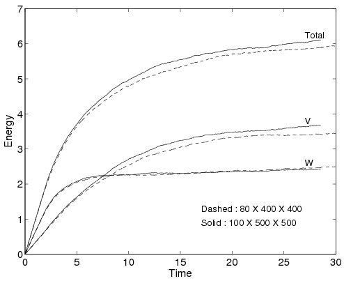
Figure 1: The wave-mode, vortical-mode and total energy vs. time for the full system. The simulations are at resolutions of $80\times 400\times 400$ and $100\times 500\times 500$ in an aspect ratio of $1/5$ and $Ro=Fr=0.05$. The runs are halted when the vortical modes near equilibration.

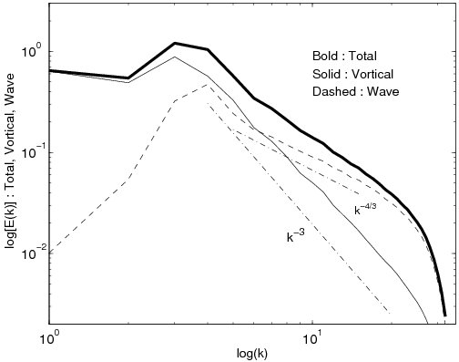
Figure 2: The wave-mode, vortical-mode and total energy spectrum (at $t\approx 28$). The results are from the $100\times 500\times 500$ run. Note that the scaling of the vortical modes is consistent with a enstrophy-cascading $k^{-3}$ form for $k_{f}<k<k_{d}$. The wave-mode spectrum is best described by a $k^{-4/3}$ scaling — we do not attribute any special significance to this number. Rather, it is drawn to show that the wave-mode scaling is consistent with a power law between $-1$ and $-5/3$.

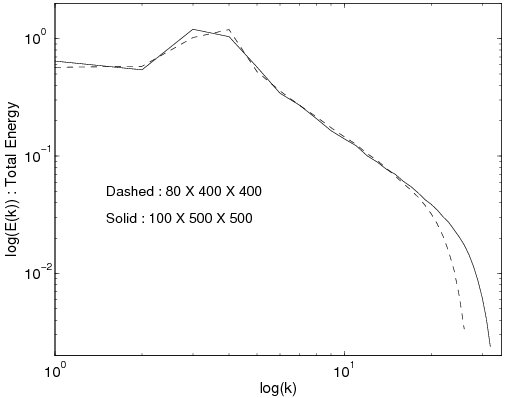
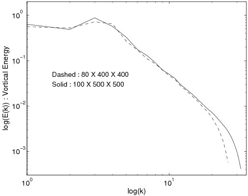
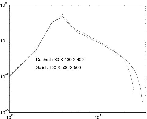
Figure 3: A comparison of the spectra for the full system at the two different resolutions. The simulations appear to have converged and are insensitive to the increasing resolution.

It is well-known that the 2D stratified problem (which only supports wave modes), on large-scale forcing, yields a clear forward transfer of energy BS ,SS . Further, the kinetic equations derived from considering resonant interactions of wave modes support power-law solutions L1 ,L2 . Keeping in mind that the GGG model can be looked upon as a 3D extension of the 2D stratified problem, these two pieces of information lead to the possibility that the GGG model will in fact support a forward transfer of energy and yield an equilibrated power-law spectrum. Forcing the GGG model with method 2, we show the total energy (equal to the wave-mode energy) vs. time in Fig. (4). Quite clearly, the energy does not equilibrate. On comparing the spectra (not shown), none of the runs showed a well-defined power-law. In essence, there is a forward transfer of energy in the GGG model, but it is highly inefficient compared to the full system forced by method 1. This inefficiency manifests itself in the lack of a systematic forward transfer and the resulting lack of an (even approximate) inertial range as is observed in the full system. For the given set of governing parameters, we speculate that the GGG model is probably under-resolved at a resolution when the full rotating Boussinesq system forced by method 1 yields consistent results across a range of resolutions.

It is interesting to observe how the presence of the interactions involving vortical modes compares to the results obtained from the GGG model when the full system is forced identically to the GGG model by method 2. Like the energy in the GGG model, the energy in the full system does not equilibriate Fig. (5). However, the full system does appear do a better job of moving the energy to small scales. After an initial growth of energy in the vortical modes ($\approx t=5$), the energy in the full system grows at a slower rate than in the GGG system. Like the GGG system, the full system now produces spectra (not shown) that are not well defined power-laws. In fact, the picture that emerges is that there is some transfer from the wave to vortical modes that results in the activation of $(w,v,w)$ interactions which help the full system move energy toward small scales. But, much like the GGG model the $(w,w,w)$ interactions are incapable of a robust forward transfer — possibily due to their being under-resolved in this set of parameters.

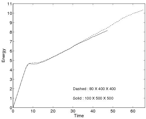
Figure 4: The total energy vs. time for the GGG model. The simulations are at resolutions of $80\times 400\times 400$ and $100\times 500\times 500$ in an aspect ratio of $1/5$ and $Ro=Fr=0.05$. Quite clearly, the system is not near equilibration; some of the runs were carried out significantly longer times and yet showed no sign of settling down. The spectra (not shown) are also evolving in time and do not show smooth power-law scaling.

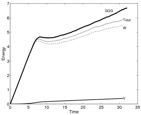
Figure 5: The total energy vs. time for the full system forced by method 2. The resolution is $100\times 500\times 500$ in an aspect ratio of $1/5$ and $Ro=Fr=0.05$. The system does not equilibriate as it did when forced by method 1. However, due to the presence of the interactions among the vortical modes it does a better job at moving energy to small scales than the identically forced GGG model does. It is possible that both systems are under-resolved in this parameter regime.

The notion that the GGG model supports a forward transfer of energy, albeit an inefficient one, but does not yield a steady state, is somewhat unsatisfactory. There is nothing intrinsically wrong with such a state of affairs, but given the possibility of their being under-resolved in the previous simulation, to gain more confidence in the GGG model we repeated the aforementioned experiment at higher $Fr,Ro$ (i.e. under weaker rotation and milder stratification) and in a less skewed domain. Specifically, setting $H/L=1/3$ and $Ro=Fr=0.1$, we performed simulations at resolutions of $144\times 432\times 432$ and $162\times 486\times 486$. Note that the aspect ratio 1/3 case allows us to use a higher numerical resolution as compared to the aspect ratio 1/5 case. Fig. (6) shows the energy in time for the GGG model forced by method 2 and the full model forced by method 1. In contrast to Fig. (4), now the GGG energy levels-off fairly rapidly. Further, as is shown in Fig. (7), the spectral distribution of the GGG energy is in the form of a smooth power-law. It is interesting to note, from Fig. (7), that the GGG spectrum is steeper than the full system’s wave-mode spectrum. In fact, this steepness is qualitatively consistent with the resonant kinetic equation solutions L1 ,L2 .

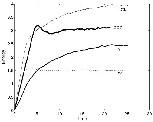
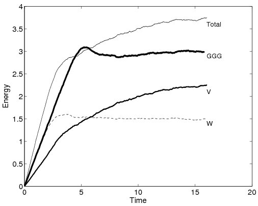
Figure 6: Left : $144\times 432\times 432$. Right : $162\times 486\times 486$. The total, vortical and wave-mode energy vs. time for the full model and the GGG model in an aspect ratio of $1/3$ with $Ro=Fr=0.1$. The behavior of the full model is similar to Fig. (1). While, in contrast to Fig. (4), now the GGG energy does level-off. Notice the agreement for both the full system and GGG between the two resolutions.

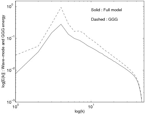
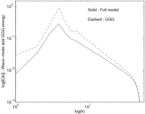
Figure 7: Left : $144\times 432\times 432$ ($\approx t=17.5s$). Right : $162\times 486\times 486$ ($\approx t=15.5s$). Wave-mode energy spectra for full and GGG models in an aspect ratio $1/3$ with $Ro=Fr=0.1$. These are spectra from a single time snapshot of the models in the quasi-statistically steady range. Quite clearly, both may be interpreted as fairly clear power-laws with the GGG model spectrum being considerably steeper than the full system’s wave-mode spectrum which scales between $-1$ and $-5/3$.

As the GGG model equilibrates in these milder conditions, it is of interest to explore the response of the full rotating Boussinesq system forced the same as the GGG model by method 2. Note that when the full system is forced by method 1 there was a natural flow of energy into the vortical mode that allowed the vortical mode to mediate energy transfer between two wave modes by means of wave-vortical-wave interactions. Given that wave to vortical transfers are weak (i.e. only due to near-resonances), forcing only the wave-modes allows us to see if the $(w,w,w)$ interactions in the full system behave in accord with the GGG model. This is precisely the case, and along with the attainment of a steady state (Fig. (8)), both simulations yield almost identical power-law wave-mode spectra for $Ro=Fr=0.1$ with $H/L=1/3$ (see Fig (9)).

In essence, this confirms our speculation that that the wave-mode interactions were under-resolved in our numerical simulations of rapid rotation and strong stratification (specifically, $Ro,Fr\leq 0.05$) in the more skewed domain ($H/L<1/5$). Quite naturally, the wave-mode energy distribution in the full rotating Boussinesq system is then primarily controlled by the $(w,w,v)$ interactions WB2 . As also noted by Waite and Bartello WB2 , our computations suggest the possibility that present-day numerical models may be deficient in their representation of $(w,w,w)$ interactions when trying to work in geophysically relevant parameter regimes. Further, in milder conditions (i.e. $Ro,Fr=0.1$ and $H/L=1/3$), the GGG model resulted in a steady state with a well-defined power-law energy distribution. This leads us to the possibility that, on proper resolution, the $(w,w,w)$ interactions may play a role in the wave-mode energy transfer and distribution in realistic parameter regimes. Future work with better computational resources will inquire into this possibility as well as universality in the GGG spectral scaling.

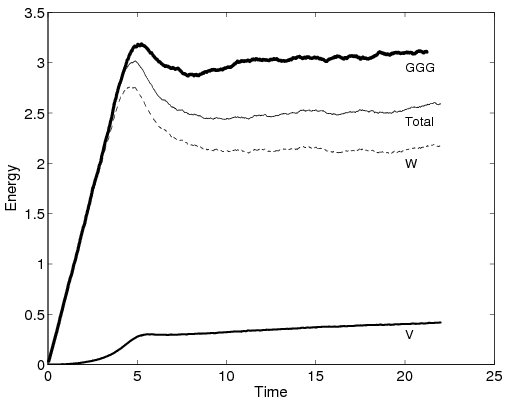
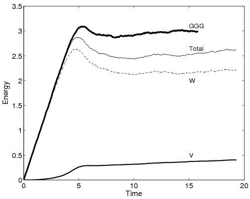
Figure 8: Left : $144\times 432\times 432$. Right : $162\times 486\times 486$. The GGG and full system wave, vortical and total energy in an aspect ratio $1/3$ and $Ro=Fr=0.1$ setting in which identical forcing by the IG modes was used. Quite clearly, both systems attain an energetically steady state. Notice the agreement for both the full system and GGG between the two resolutions.

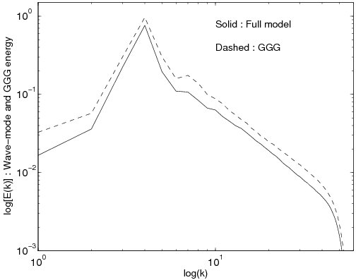
Figure 9: Left : $144\times 432\times 432$ ($\approx t=18.65s$). Right : $162\times 486\times 486$ ($\approx t=17.7s$). The GGG and full system wave-mode energy spectrum in an aspect ratio $1/3$ and $Ro=Fr=0.1$ setting in which identical forcing by the IG modes was used. These are spectra from a single time snapshot of the models. Quite clearly, both may be interpreted as fairly consistent power-laws.

IV Conclusions

In rotating and stratified flows, the forward transfer and distribution of energy among wave modes is controlled primarily by wave-vortical-wave $(w,w,v)$ and wave-wave-wave $(w,w,w)$ interactions. However, the relative importance of these two classes of interactions is somewhat unclear. On one hand, prior analytical Babin-rev and numerical Bartello ,SS-gafd work suggests that the wave-vortical-wave class of interactions is of primary importance — when $1/2\leq f/N\leq 2$, this is immediately evident WB2 . On the other hand, especially outside the range $1/2\leq f/N\leq 2$ (as is true in most geophysical scenarios), the kinetic equation approach considering only resonant IG wave-mode interactions yields solutions that are consistent with certain observations L1 ,L2 . In order to inquire into this somewhat dichotomous situation, we constructed a reduced model consisting only of wave-mode interactions (resonant and non-resonant). This GGG model is given by a PDE that conserves energy in the inviscid, unforced case. We studied the GGG model in an idealized periodic setting, though its applicability is not limited to such idealized domains.

We compared the GGG model to the full system in a geophysically relevant parameter regime. Specifically, with a skewed aspect ratio $H/L<1$, we chose $f,N$ such that $Ro=Fr\Rightarrow Bu=1$. Further, the flow was rapidly rotating and strongly stratified, i.e. $Fr=Ro\ll 1$. In the full system, as anticipated we observed an inverse transfer of energy among the vortical modes accompanying by a power-law that was consistent with a $k^{-3}$ scaling for $k_{f}<k<k_{d}$. The wave-mode energy was transferred to small scales, and these modes equilibrated quite rapidly. In accord with prior work Bartello ,SS-gafd ,Kitamura , the wave-mode energy distribution was consistent with a power law with scaling between a $k^{-1}$ to $k^{-5/3}$ form for $k_{f}<k<k_{d}$.

For the GGG model, we also anticipated a statistically steady wave-mode energy spectrum with power-law scaling. This expectation follows from previous results establishing that (i) power-law solutions are supported by the kinetic equations governing resonant wave-mode interactions, and (ii) the GGG model is a 3D extension of the 2D stratified problem (known to support a robust forward transfer of energy). A clear power law was indeed observed for ”mild” conditions with $H/L=1/3$ and $Fr=Ro\approx 0.1$. Consistent with the kinetic equations for resonant wave interactions, the GGG energy spectra were observed to be steeper than the wave-mode energy spectra associated with the full equations when all modes were forced with equal weight. When the forcing was restricted to excite only wave modes, then the GGG and full systems yielded wave-mode spectra with essentially identical power-law scaling. The results indicate that $(w,w,w)$ interactions can play a significant role in the transfer of energy from forced scales to smaller scales, especially when the wave modes are preferentially excited. However, the energy did not equilibrate for the GGG flow in the smaller aspect ratio $H/L=1/5$ with stronger rotation and stratification ($Fr=Ro=0.05$), suggesting an in-efficient forward transfer of energy. Furthermore, the full system also did not equilibrate for these parameter values when only the wave modes were excited at large scales. These results serve as a caution that improper resolution of wave-mode interactions may be a significant issue in present-day numerical models that attempt to work in geophysically relevant parameter regimes, consistent with WB2 . Finally, there are a number of issues that raised herein that we feel merit further examination. For example, is there universality in the wave-mode spectrum from the GGG model (with respect to decreasing $Fr=Ro$ in a fixed aspect ratio). Similarly, with better numerical resources, an important issue to be addressed is the difference in scaling of the wave-mode energy from full model simulations (with forcing of type 1) and that from the GGG model. This gets to the heart of the matter with regard to energy distribution resulting from $(w,v,w)$ and $(w,w,w)$ interactions respectively — indeed, the intriguing possibility that the scaling from these two scenarios may converge with progressively stronger rotation and stratification provides adequate motivation for such an exploration.

Acknowledgements : Financial support was provided by NSF CMG 0529596 and the DOE Multiscale Mathematics program (DE-FG02-05ER25703).

V Appendix

Here we present the GGG model by utilizing the eigenfunction decomposition suggested in (3). For the general case, i.e. $k_{x},k_{y},k_{z}\neq 0$, the eigenfunctions are

$$\phi^{+}=\frac{1}{\sqrt{2}\sigma_{k}k}\left(\begin{array}[]{c}\frac{k_{z}}{k_{h}}(\sigma_{k}k_{x}+{\rm i}k_{y}f)\\ \frac{k_{z}}{k_{h}}(\sigma_{k}k_{y}-{\rm i}k_{x}f)\\ -\sigma_{k}k_{h}\\ -{\rm i}Nk_{h}\end{array}\right),\quad\phi^{-}={\phi^{+}}^{*},\quad\phi^{0}=\frac{1}{\sigma_{k}k}\left(\begin{array}[]{c}Nk_{y}\\ -Nk_{x}\\ 0\\ fk_{z}\end{array}\right)$$ (37)

here ${(\cdot)}^{*}$ denotes complex-conjugate. The special case, $k_{h}=0,k_{z}\neq 0$ (the VSHF mode) is treated separately. Here $\sigma^{0}=0,~{}\sigma^{\pm}(\mathbf{k})=\pm f$ and

$$\phi^{+}=\left(\begin{array}[]{c}\frac{{\rm i}}{\sqrt{2}}\\ \frac{1}{\sqrt{2}}\\ 0\\ 0\end{array}\right),\quad\phi^{-}={\phi^{+}}^{*},\quad\phi^{0}=\left(\begin{array}[]{c}0\\ 0\\ 0\\ \text{sgn}(fk_{z})\end{array}\right)$$ (46)

or,

$$\phi^{+}=\frac{1}{2}\left(\begin{array}[]{c}1+{\rm i}\\ 1-{\rm i}\\ 0\\ 0\end{array}\right),\quad\phi^{-}={\phi^{+}}^{*},\quad\phi^{0}=\left(\begin{array}[]{c}0\\ 0\\ 0\\ \text{sgn}(fk_{z})\end{array}\right)$$ (55)

Substituting in (3) and using the orthogonality of the modes, with $\psi$ as the streamfunction, we have

• For $k_{x},k_{y},k_{z}\neq 0$ :

  $$a_{k}^{0}=\frac{{\rm i}N}{\sigma_{k}k}(-k_{h}^{2}\psi-{\rm i}\frac{f}{N}k_{z}\theta)$$

  $$a_{k}^{+}=\frac{1}{\sqrt{2}\sigma_{k}k}(-\frac{\sigma_{k}w_{k}k^{2}}{k_{h}}-fk_{z}k_{h}\psi+{\rm i}Nk_{h}\theta)$$

  $$a_{k}^{-}=\frac{1}{\sqrt{2}\sigma_{k}k}(-\frac{\sigma_{k}w_{k}k^{2}}{k_{h}}+fk_{z}k_{h}\psi-{\rm i}Nk_{h}\theta)$$

  $$a_{k}^{+}+a_{k}^{-}=-\frac{\sqrt{2}kw_{k}}{k_{h}}$$

  $$a_{k}^{+}-a_{k}^{-}=\frac{\sqrt{2}{\rm i}fk_{h}}{\sigma_{k}k}(\frac{N}{f}\theta+{\rm i}k_{z}\psi)$$ (56)

• For $k_{h}=0,k_{z}\neq 0$ :

  $$a_{k_{z}}^{0}=\overline{\theta(z)}\text{sgn}(fk_{z})\quad a_{k_{z}}^{+}=\frac{-{\rm i}\overline{u}+\overline{v}}{\sqrt{2}}\quad a_{k_{z}}^{-}=\frac{{\rm i}\overline{u}+\overline{v}}{\sqrt{2}}$$

  $$(a^{+}_{k_{z}}+a^{-}_{k_{z}})=\sqrt{2}\overline{v(z)}\qquad(a^{+}_{k_{z}}-a^{-}_{k_{z}})=-{\rm i}\sqrt{2}\overline{u(z)}$$ (57)

  where $\overline{(\cdot)}$ denotes a horizontal average.

Using (37) and (56), the GGG model (retaining only IG mode interactions) for the $k_{x},k_{y},k_{z}\neq 0$ case is

$$\frac{\partial(a_{\mathbf{k}}^{+}+a_{\mathbf{k}}^{-})}{\partial t} +{\rm i}\sigma_{\mathbf{k}}(a^{+}_{\mathbf{k}}-a^{-}_{\mathbf{k}})=\sum_{\mathbf{k}=\mathbf{p}+\mathbf{q}}\frac{1}{\sqrt{2}\sigma_{k}k}\Bigg{\{}(\frac{a_{\mathbf{p}}^{+}+a_{\mathbf{p}}^{-}}{\sigma_{p}p})\left(\frac{a_{\mathbf{q}}^{+}+a_{\mathbf{q}}^{-}}{\sigma_{q}q}\right)\Big{\{}\frac{{\rm i}\sigma_{p}\sigma_{q}\sigma_{k}p_{h}^{2}q_{h}^{2}p_{z}^{3}}{p_{h}q_{h}k_{h}}$$ (58)

$$+\frac{{\rm i}\sigma_{p}\sigma_{q}\sigma_{k}p_{h}^{2}q_{h}^{2}p_{z}q_{z}^{2}}{p_{h}q_{h}k_{h}}+\frac{{\rm i}\sigma_{p}\sigma_{q}\sigma_{k}(\mathbf{p}_{h}\cdot\mathbf{q}_{h})q_{h}^{2}p_{z}^{3}}{p_{h}q_{h}k_{h}}-\frac{{\rm i}\sigma_{p}\sigma_{q}\sigma_{k}(\mathbf{p}_{h}\cdot\mathbf{q}_{h})q_{h}^{2}p_{z}q_{z}^{2}}{p_{h}q_{h}k_{h}})$$

$$-2\frac{{\rm i}\sigma_{p}\sigma_{q}\sigma_{k}(\mathbf{p}_{h}\cdot\mathbf{q})^{2}p_{z}q_{z}^{2}}{p_{h}q_{h}k_{h}}+{\rm i}\sigma_{p}\sigma_{q}\sigma_{k}p_{h}q_{h}k_{h}p_{z}-{\rm i}\sigma_{p}\sigma_{q}\sigma_{k}(\mathbf{p}_{h}\cdot\mathbf{q}_{h})\frac{q_{h}}{p_{h}}p_{z}\}\Big{\}}$$

$$+\left(\frac{a_{\mathbf{p}}^{+}+a_{\mathbf{p}}^{-}}{\sigma_{p}p}\right)\left(\frac{a_{\mathbf{q}}^{+}-a_{\mathbf{q}}^{-}}{\sigma_{q}q}\right)\Big{\{}2\frac{f\sigma_{k}\sigma_{p}(\mathbf{p}\times\mathbf{q}\cdot\hat{z})(\mathbf{p}_{h}\cdot\mathbf{q}_{h})(p_{z}^{2}q_{z}+p_{z}q_{z}^{2})}{p_{h}q_{h}k_{h}}$$

$$-\frac{f\sigma_{p}\sigma_{k}q_{z}^{3}(\mathbf{p}\times\mathbf{q}\cdot\hat{z})p_{h}^{2}}{p_{h}q_{h}k_{h}}+\frac{f\sigma_{k}\sigma_{p}p_{z}^{2}q_{z}(\mathbf{p}\times\mathbf{q}\cdot\hat{z})p_{h}^{2}}{p_{h}q_{h}k_{h}}+f\sigma_{k}\sigma_{p}k_{h}(\mathbf{p}\times\mathbf{q}\cdot\hat{z})\frac{p_{h}}{q_{h}}q_{z}\Big{\}}$$

$$+\left(\frac{a_{\mathbf{p}}^{+}-a_{\mathbf{p}}^{-}}{\sigma_{p}p}\right)\left(\frac{a_{\mathbf{q}}^{+}-a_{\mathbf{q}}^{-}}{\sigma_{q}q}\right)\Big{\{}-2\frac{{\rm i}f^{2}\sigma_{k}(\mathbf{p}\times\mathbf{q}\cdot\hat{z})^{2}p_{z}^{2}q_{z}}{p_{h}q_{h}k_{h}}\Big{\}}\Bigg{\}}$$

and

$$\frac{\partial(a_{\mathbf{k}}^{+}-a_{\mathbf{k}}^{-})}{\partial t} +{\rm i}\sigma_{\mathbf{k}}(a^{+}_{\mathbf{k}}+a^{-}_{\mathbf{k}})=\sum_{\mathbf{k}=\mathbf{p}+\mathbf{q}}\frac{1}{2\sqrt{2}\sigma_{k}k}\Bigg{\{}\left(\frac{a_{\mathbf{p}}^{+}+a_{\mathbf{p}}^{-}}{\sigma_{p}p}\right)\left(\frac{a_{\mathbf{q}}^{+}+a_{\mathbf{q}}^{-}}{\sigma_{q}q}\right)\Big{\{}\frac{f\sigma_{p}\sigma_{q}(\mathbf{p}\times\mathbf{q}\cdot\hat{z})p_{z}^{3}q_{h}^{2}}{p_{h}q_{h}k_{h}}$$ (59)

$$+\frac{f\sigma_{p}\sigma_{q}(\mathbf{p}\times\mathbf{q}\cdot\hat{z})p_{z}^{2}q_{z}q_{h}^{2}}{p_{h}q_{h}k_{h}}\Big{\}}+\left(\frac{a_{\mathbf{p}}^{+}+a_{\mathbf{p}}^{-}}{\sigma_{p}p}\right)\left(\frac{a_{\mathbf{q}}^{+}-a_{\mathbf{q}}^{-}}{\sigma_{q}q}\right)\Big{\{}-\frac{{\rm i}f^{2}\sigma_{p}p_{z}^{2}q_{z}p_{h}^{2}q_{h}^{2}}{p_{h}q_{h}k_{h}}-\frac{{\rm i}f^{2}\sigma_{p}p_{z}^{2}q_{z}(\mathbf{p}_{h}\cdot\mathbf{q}_{h})q_{h}^{2}}{p_{h}q_{h}k_{h}}$$

$$-\frac{{\rm i}f^{2}\sigma_{p}p_{z}q_{z}^{2}(\mathbf{p}_{h}\cdot\mathbf{q}_{h})q_{h}^{2}}{p_{h}q_{h}k_{h}}+\frac{{\rm i}f^{2}\sigma_{p}q_{z}^{3}p_{h}^{2}q_{h}^{2}}{p_{h}q_{h}k_{h}}+\frac{{\rm i}f^{2}\sigma_{p}p_{z}q_{z}^{2}(\mathbf{p}_{h}\cdot\mathbf{q}_{h})p_{h}^{2}}{p_{h}q_{h}k_{h}}+\frac{{\rm i}f^{2}\sigma_{p}q_{z}^{3}(\mathbf{p}_{h}\cdot\mathbf{q}_{h})p_{h}^{2}}{p_{h}q_{h}k_{h}}$$

$$-{\rm i}N^{2}k_{h}(\mathbf{p}_{h}\cdot\mathbf{q}_{h})\frac{q_{h}}{p_{h}}p_{z}\sigma_{p}+{\rm i}N^{2}p_{h}q_{h}k_{h}q_{z}\sigma_{p}\Big{\}}+\left(\frac{a_{\mathbf{p}}^{+}-a_{\mathbf{p}}^{-}}{\sigma_{p}p}\right)\left(\frac{a_{\mathbf{q}}^{+}-a_{\mathbf{q}}^{-}}{\sigma_{q}q}\right)\Big{\{}$$

$$+\frac{f^{3}(\mathbf{p}\times\mathbf{q}\cdot\hat{z})p_{z}^{2}q_{z}p_{h}^{2}}{p_{h}q_{h}k_{k}}+\frac{f^{3}(\mathbf{p}\times\mathbf{q}\cdot\hat{z})p_{z}q_{z}^{2}p_{h}^{2}}{p_{h}q_{h}k_{k}}+fN^{2}k_{h}(\mathbf{p}\times\mathbf{q}\cdot\hat{z})q_{z}\frac{p_{h}}{q_{h}}\Big{\}}\Bigg{\}}$$

The VSHF contributions to the above are

$$\frac{\partial(a_{\mathbf{k}}^{+}+a_{\mathbf{k}}^{-})}{\partial t} +{\rm i}\sigma_{\mathbf{k}}(a^{+}_{\mathbf{k}}-a^{-}_{\mathbf{k}})=\sum_{k_{z}=p_{z}+q_{z},k_{h}=q_{h}}\frac{1}{\sqrt{2}k}\Big{\{}(a^{+}_{p_{z}}+a^{-}_{p_{z}})(\frac{a_{\mathbf{q}}^{+}+a_{\mathbf{q}}^{-}}{q})({\rm i}q_{y}p_{z}^{2}-{\rm i}q_{y}q_{z}^{2}-{\rm i}q_{y}q_{h}^{2})$$ (60)

$$+(a^{+}_{p_{z}}-a^{-}_{p_{z}})(\frac{a_{\mathbf{q}}^{+}+a_{\mathbf{q}}^{-}}{q})(-q_{x}p_{z}^{2}+q_{x}q_{z}^{2}+q_{x}q_{h}^{2})\Big{\}}$$

and

$$\frac{\partial(a_{\mathbf{k}}^{+}-a_{\mathbf{k}}^{-})}{\partial t} +{\rm i}\sigma_{\mathbf{k}}(a^{+}_{\mathbf{k}}+a^{-}_{\mathbf{k}})=\sum_{k_{z}=p_{z}+q_{z},k_{h}=q_{h}}\frac{1}{\sqrt{2}\sigma_{k}k}\Big{\{}(a^{+}_{p_{z}}+a^{-}_{p_{z}})(\frac{a_{\mathbf{q}}^{+}+a_{\mathbf{q}}^{-}}{q})(-fq_{x}p_{z}(p_{z}+q_{z})$$ (61)

$$+(a^{+}_{p_{z}}-a^{-}_{p_{z}})(\frac{a_{\mathbf{q}}^{+}+a_{\mathbf{q}}^{-}}{q})({\rm i}fq_{y}p_{z}(p_{z}+q_{z}))+(a^{+}_{p_{z}}+a^{-}_{p_{z}})(\frac{a_{\mathbf{q}}^{+}-a_{\mathbf{q}}^{-}}{\sigma_{q}q})(-{\rm i}f^{2}q_{y}q_{z}(p_{z}+q_{z})$$

$$-{\rm i}N^{2}q_{y}q_{h}^{2})+(a^{+}_{p_{z}}-a^{-}_{p_{z}})(\frac{a_{\mathbf{q}}^{+}-a_{\mathbf{q}}^{-}}{q\sigma_{q}})(f^{2}q_{x}q_{z}(p_{z}+q_{z})+N^{2}q_{y}q_{h}^{2})\Big{\}}$$

and finally, using (46) and (58), the evolution the VSHF modes themselves is given by

$$\frac{\partial(a^{+}_{k_{z}}+a^{-}_{k_{z}})}{\partial t}+{\rm i}\sigma_{k_{z}}(a^{+}_{k_{z}}-a^{-}_{k_{z}}) =-\sum_{k_{z}=p_{z}+q_{z},\mathbf{p_{h}}}\frac{1}{2\sqrt{2}}\Bigg{\{}(\frac{a^{+}_{p}+a^{-}_{p}}{p})(\frac{a^{+}_{\mathbf{p_{h}},qz}+a^{-}_{\mathbf{p_{h}},qz}}{q})({\rm i}p_{y}(q_{z}^{2}-p_{z}^{2})$$ (62)

$$+(\frac{a_{p}^{+}-a_{p}^{-}}{\sigma_{p}p})(\frac{a^{+}_{\mathbf{p_{h}},qz}+a^{-}_{\mathbf{p_{h}},qz}}{q})(-fp_{x}p_{z}q_{z}-fp_{x}p_{z}^{2})$$

$$+(\frac{a_{p}^{+}+a_{p}^{-}}{p})(\frac{a^{+}_{\mathbf{p_{h}},qz}-a^{-}_{\mathbf{p_{h}},qz}}{\sigma_{q}q})(fp_{x}p_{z}q_{z}+fp_{x}q_{z}^{2})\Bigg{\}}$$

and

$$\frac{\partial(a^{+}_{k_{z}}-a^{-}_{k_{z}})}{\partial t}+{\rm i}\sigma_{k_{z}}(a^{+}_{k_{z}}+a^{-}_{k_{z}}) =-\sum_{k_{z}=p_{z}+q_{z},\mathbf{p_{h}}}\frac{1}{2\sqrt{2}}\Bigg{\{}(\frac{a^{+}_{p}+a^{-}_{p}}{p})(\frac{a^{+}_{\mathbf{p_{h}},qz}+a^{-}_{\mathbf{p_{h}},qz}}{q})p_{x}(q_{z}^{2}-p_{z}^{2})$$ (63)

$$+(\frac{a_{p}^{+}-a_{p}^{-}}{\sigma_{p}p})(\frac{a^{+}_{\mathbf{p_{h}},qz}+a^{-}_{\mathbf{p_{h}},qz}}{q})(-{\rm i}p_{y}f(p_{z}^{2}+p_{z}q_{z}))$$

$$+(\frac{a_{p}^{+}+a_{p}^{-}}{p})(\frac{a^{+}_{\mathbf{p_{h}},qz}-a^{-}_{\mathbf{p_{h}},qz}}{\sigma_{q}q}){\rm i}p_{y}f(q_{z}^{2}+p_{z}q_{z})\Bigg{\}}.$$

It can be verified that inverse transforming these equations leads to exactly the set specified in Section IIB.

References

- (1) A.E. Gill, Atmosphere-Ocean Dynamics, Academic Press, International Geophysics Series, Vol. 30 1982.
- (2) C. Garrett and W. Munk, ”Internal waves in the ocean,” Annu. Rev. Fluid Mech. 11, 339 (1979).
- (3) K.L. Polzin and Y.V. Lvov, ”Toward regional characterizations of the oceanic internal wavefield,” submitted to Rev. Geophys (2008).
- (4) C. Staquet and J. Sommeria, ”Internal gravity waves: From instabilities to turbulence,” Annu. Rev. Fluid Mech. 34, 559 (2002).
- (5) C. Wunsch and R. Ferrari, ”Vertical mixing, energy and the general circulation of the oceans,” Annu. Rev. Fluid Mech. 36, 281 (2004).
- (6) D. Fritts and J. Alexander, ”Gravity wave dynamics and effects in the middle atmosphere,” Rev. Geophys. 41, art. no. 1001 (2003).
- (7) C. Garrett and W. Munk, ”Space-time scales of internal waves,” Geophys. Fluid Dynamics, 2, 225 (1972).
- (8) C.H. McComas and F.P. Bretherton, ”Resonant interaction of oceanic internal waves,” J. Geophys. Res. 82, 1397 (1977).
- (9) A.M. Anile, J.K. Hunter, P. Pantano and G. Russo, Ray methods for nonlinear waves in fluids and plasmas, John Wiley and Sons NY, Pitman Monographs and Surveys in Pure and Applied Mathematics 57 (1993).
- (10) V. Zakharov, V. Lvov, G. Falkovich, Kolmogorov Spectra of Turbulence, Springer, Berlin, 1992
- (11) A.J. Majda, Introduction to PDEs and Waves for the Atmosphere and Ocean, American Mathematical Society (2003).
- (12) J-Y. Chemin et al. Mathematical Geophysics, Oxford Lecture Series in Mathematics and its Applications, Vol. 32, Oxford University Press, UK (2006).
- (13) P. Bartello, ”Geostrophic adjustment and inverse cascades in rotating stratified turbulence,” J. Atmos. Sci. 52, 4410 (1995).
- (14) J. Sukhatme and L.M. Smith, ”Vortical and Wave Modes in 3D Rotating Stratified Flows : Random Large Scale Forcing,” Geophys. Astrophys. Fluid Dynamics, 102, 437 (2008).
- (15) P. Muller, G. Holloway, F. Henyey and N. Pomphrey, ”Nonlinear interactions amongst internal gravity waves,” Rev. Geophys. 24, 493 (1986).
- (16) Y.V. Lvov, K.L. Polzin and N. Yokoyama, ”Wave-wave interactions in stratified fluids: A comparison between different approaches,” available online at arxiv.org/abs/0706.3712 (2008).
- (17) Y.V. Lvov and E.G. Tabak, ”Hamiltonian formalism and the Garrett-Munk spectrum of internal waves in the ocean,” Phys. Rev. Lett. 87, 168501 (2001).
- (18) Y.V. Lvov, K.L. Polzin and E.G. Tabak, ”Energy spectra of the ocean’s internal wave field: Theory and observations,” Phys. Rev. Lett. 92, 128501 (2004).
- (19) A. Babin, A. Mahalov and B. Nicolaenko, ”Singular oscillating limits of stably-stratified 3D Euler and Navier-Stokes equations and ageostrophic wave fronts,” in Large-Scale Atmosphere-Ocean Dynamics I, eds. J. Norbury and I. Roulstone, Cambridge University Press (2002).
- (20) P. Bouruet-Aubertot, J. Sommeria and C. Staquet, ”Breaking of standing internal gravity waves through two-dimensional instabilities,” J. Fluid. Mech. 285, 265 (1995).
- (21) J. Sukhatme and L.M. Smith, ”Self-similarity in decaying two-dimensional stably stratified adjustment,” Phys. of Fluids, 19, 036603 (2007).
- (22) L.M. Smith, ”Numerical study of two-dimensional stratified turbulence,” Contemporary Mathematics, 283, 91 (2001).
- (23) M.-P. Lelong and J. Riley, ”Internal wave-vortical mode interactions in strongly stratified flows,” J. Fluid. Mech. 232, 1 (1991).
- (24) L.M. Smith and F. Waleffe, ”Generation of slow large-scales in forced rotating stratified turbulence,” J. Fluid. Mech. 451, 145 (2002).
- (25) P.F. Embid and A.J. Majda, ”Low Froude number limiting dynamics for stably stratified flow with small or finite Rossby numbers,” Geophys. Astrophys. Fluid Dynamics, 87, 1 (1998).
- (26) P.F. Embid and A.J. Majda, ”Averaging over wave gravity waves for geophysical flows with arbitrary potential vorticity,” Commun. in Partial Differential Equations, 21, 619 (1996).
- (27) A.J. Majda and P.F. Embid, ”Averaging over fast waves for geophysical flows with unbalanced initial data,” Theor. Comp. Flu. Dyn. 11, 155 (1998).
- (28) J.-P. Laval, J. C. McWilliams and B. Dubrulle, ”Forced stratified turbulence: Successive transitions with Reynolds number,” Phys. Rev. E 68, 036308 (2003).
- (29) M.L. Waite and P. Bartello, ”Stratified turbulence dominated by vortical motion,” J. Fluid. Mech. 517 281 (2004).
- (30) M.L. Waite and P. Bartello, ”Stratified turbulence generated by internal gravity waves,” J. Fluid. Mech. 546 313 (2006).
- (31) L.M. Smith and Y. Lee, ”On near resonances and symmetry breaking in forced rotating flows at moderate Rossby number,” J. Fluid. Mech. 535, 111 (2005).
- (32) S.Y. Annenkov and V.I. Shrira, ”Role of non-resonant interactions in the evolution of nonlinear random water wave fields,” J. Fluid. Mech. 561, 181 (2006).
- (33) K.M. Watson and S.B. Buchsbaum, ”Interaction of capillary waves with longer waves .1. General theory and specific applications to waves in one dimension,” J. Fluid. Mech. 321, 87 (1996).
- (34) R.H. Kraichnan, ”Helical turbulence and absolute equilibrium,” J. Fluid. Mech. 59 745 (1973).
- (35) M. Remmel and L.M. Smith, ”New Intermediate Models for Rotating Shallow Water and an Investigation for the Preference for Anticyclones,” submitted to J. Fluid. Mech. (2008).
- (36) Y. Kitamura and Y. Matsuda, ”The and energy spectra in stratified turbulence,” Geophys. Res. Lett. 33, L05809 (2006).