Abstract

In this article, we perform a systematic study of the mass spectrum of the vector hidden charm and bottom tetraquark states using the QCD sum rules.

PACS number: 12.39.Mk, 12.38.Lg

Key words: Tetraquark state, QCD sum rules

1 Introduction

The Babar, Belle, CLEO, D0, CDF and FOCUS collaborations have discovered (or confirmed) a large number of charmonium-like states, such as $X(3940)$, $X(3872)$, $Y(4260)$, $Y(4008)$, $Y(3940)$, $Y(4325)$, $Y(4360)$, $Y(4660)$, etc, and revitalized the interest in the spectroscopy of the charmonium states [1, 2, 3, 4, 5]. Many possible assignments for those states have been suggested, such as multiquark states (irrespective of the molecule type and the diquark-antidiquark type), hybrid states, charmonium states modified by nearby thresholds, threshold cusps, etc [1, 2, 3, 4].

The $Z^{+}(4430)$ observed in the decay mode $\psi^{\prime}\pi^{+}$ by the Belle collaboration is the most interesting subject [6]. We can distinguish the multiquark states from the hybrids or charmonia with the criterion of non-zero charge. The $Z^{+}(4430)$ can’t be a pure $c\bar{c}$ state due to the positive charge, and may be a $c\bar{c}u\bar{d}$ tetraquark state. However, the Babar collaboration did not confirm this resonance [7]. The two resonance-like structures $Z(4050)$ and $Z(4250)$ in the $\pi^{+}\chi_{c1}$ invariant mass distribution near $4.1\,\rm{GeV}$ are also particularly interesting [8]. Their quark contents must be some special combinations of the $c\bar{c}u\bar{d}$, just like the $Z^{+}(4430)$, they can’t be the conventional mesons.

In Refs.[9, 10], we assume that the hidden charm mesons $Z(4050)$ and $Z(4250)$ are vector (and scalar) tetraquark states, and study their masses using the QCD sum rules. The numerical results indicate that the mass of the vector hidden charm tetraquark state is about $M_{Z}=(5.12\pm 0.15)\,\rm{GeV}$ or $M_{Z}=(5.16\pm 0.16)\,\rm{GeV}$, while the mass of the scalar hidden charm tetraquark state is about $M_{Z}=(4.36\pm 0.18)\,\rm{GeV}$. The resonance-like structure $Z(4250)$ observed by the Belle collaboration in the $\pi^{+}\chi_{c1}$ invariant mass distribution near $4.1\,\rm{GeV}$ in the exclusive decays $\bar{B}^{0}\to K^{-}\pi^{+}\chi_{c1}$ can be tentatively identified as the scalar tetraquark state [10]. In Ref.[11], we study the mass spectrum of the scalar hidden charm and bottom tetraquark states using the QCD sum rules. In this article, we extend our previous work to study the mass spectrum of the vector hidden charm and bottom tetraquark states.

In the QCD sum rules, the operator product expansion is used to expand the time-ordered currents into a series of quark and gluon condensates which parameterize the long distance properties of the QCD vacuum. Based on the quark-hadron duality, we can obtain copious information about the hadronic parameters at the phenomenological side [12, 13].

The mass is a fundamental parameter in describing a hadron, whether or not there exist those hidden charm or bottom tetraquark configurations is of great importance itself, because it provides a new opportunity for a deeper understanding of the low energy QCD. The vector hidden charm ($c\bar{c}$) and bottom ($b\bar{b}$) tetraquark states may be observed at the LHCb, where the $b\bar{b}$ pairs will be copiously produced with the cross section about $500\,\mu b$ [14].

The hidden charm and bottom tetraquark states ($Z$) have the symbolic quark structures:

$$Z^{+}=Q\bar{Q}u\bar{d};~{}~{}~{}~{}Z^{0}=\frac{1}{\sqrt{2}}Q\bar{Q} (u\bar{u}-d\bar{d});~{}~{}~{}~{}Z^{-}=Q\bar{Q}d\bar{u};$$

$$Z_{s}^{+}=Q\bar{Q}u\bar{s};~{}~{}~{}~{}Z_{s}^{-}=Q\bar{Q}s\bar{u}; ~{}~{}~{}~{}Z_{s}^{0}=Q\bar{Q}d\bar{s};~{}~{}~{}~{}\overline{Z}_{s}^{0}=Q\bar{Q}s\bar{d};$$

$$Z_{\varphi}=\frac{1}{\sqrt{2}}Q\bar{Q}(u\bar{u}+d\bar{d}); ~{}~{}~{}~{}Z_{\phi}=Q\bar{Q}s\bar{s}\,,$$ (1)

where the $Q$ denote the heavy quarks $c$ and $b$.

We take the diquarks as the basic constituents following Jaffe and Wilczek [15, 16], and construct the tetraquark states with the diquark and antidiquark pairs. The diquarks have five Dirac tensor structures, scalar $C\gamma_{5}$, pseudoscalar $C$, vector $C\gamma_{\mu}\gamma_{5}$, axial vector $C\gamma_{\mu}$ and tensor $C\sigma_{\mu\nu}$, where $C$ is the charge conjunction matrix. The structures $C\gamma_{\mu}$ and $C\sigma_{\mu\nu}$ are symmetric, the structures $C\gamma_{5}$, $C$ and $C\gamma_{\mu}\gamma_{5}$ are antisymmetric. The attractive interactions of one-gluon exchange favor formation of the diquarks in color antitriplet $\overline{3}_{c}$, flavor antitriplet $\overline{3}_{f}$ and spin singlet $1_{s}$ [17, 18]. In this article, we assume the vector hidden charm and bottom mesons $Z$ consist of the $C\gamma_{5}-C\gamma_{\mu}\gamma_{5}$ type and $C-C\gamma_{\mu}$ type diquark structures, and construct the interpolating currents $J^{\mu}(x)$ and $\eta^{\mu}(x)$:

$$J^{\mu}_{Z^{+}}(x) = \epsilon^{ijk}\epsilon^{imn}u_{j}^{T}(x)C\gamma_{5}Q_{k}(x)\bar{Q}_{m}(x)\gamma_{5}\gamma^{\mu}C\bar{d}_{n}^{T}(x)\,,$$

$$J^{\mu}_{Z^{0}}(x) = \frac{\epsilon^{ijk}\epsilon^{imn}}{\sqrt{2}}\left[u_{j}^{T}(x)C\gamma_{5}Q_{k}(x)\bar{Q}_{m}(x)\gamma_{5}\gamma^{\mu}C\bar{u}_{n}^{T}(x)-(u\rightarrow d)\right]\,,$$

$$J^{\mu}_{Z^{+}_{s}}(x) = \epsilon^{ijk}\epsilon^{imn}u_{j}^{T}(x)C\gamma_{5}Q_{k}(x)\bar{Q}_{m}(x)\gamma_{5}\gamma^{\mu}C\bar{s}_{n}^{T}(x)\,,$$

$$J^{\mu}_{Z^{0}_{s}}(x) = \epsilon^{ijk}\epsilon^{imn}d_{j}^{T}(x)C\gamma_{5}Q_{k}(x)\bar{Q}_{m}(x)\gamma_{5}\gamma^{\mu}C\bar{s}_{n}^{T}(x)\,,$$

$$J^{\mu}_{Z_{\varphi}}(x) = \frac{\epsilon^{ijk}\epsilon^{imn}}{\sqrt{2}}\left[u_{j}^{T}(x)C\gamma_{5}Q_{k}(x)\bar{Q}_{m}(x)\gamma_{5}\gamma^{\mu}C\bar{u}_{n}^{T}(x)+(u\rightarrow d)\right]\,,$$

$$J^{\mu}_{Z_{\phi}}(x) = \epsilon^{ijk}\epsilon^{imn}s_{j}^{T}(x)C\gamma_{5}Q_{k}(x)\bar{Q}_{m}(x)\gamma_{5}\gamma^{\mu}C\bar{s}_{n}^{T}(x)\,,$$

$$\eta^{\mu}_{Z^{+}}(x) = \epsilon^{ijk}\epsilon^{imn}u_{j}^{T}(x)CQ_{k}(x)\bar{Q}_{m}(x)\gamma^{\mu}C\bar{d}_{n}^{T}(x)\,,$$

$$\eta^{\mu}_{Z^{0}}(x) = \frac{\epsilon^{ijk}\epsilon^{imn}}{\sqrt{2}}\left[u_{j}^{T}(x)CQ_{k}(x)\bar{Q}_{m}(x)\gamma^{\mu}C\bar{u}_{n}^{T}(x)-(u\rightarrow d)\right]\,,$$

$$\eta^{\mu}_{Z^{+}_{s}}(x) = \epsilon^{ijk}\epsilon^{imn}u_{j}^{T}(x)CQ_{k}(x)\bar{Q}_{m}(x)\gamma^{\mu}C\bar{s}_{n}^{T}(x)\,,$$

$$\eta^{\mu}_{Z^{0}_{s}}(x) = \epsilon^{ijk}\epsilon^{imn}d_{j}^{T}(x)CQ_{k}(x)\bar{Q}_{m}(x)\gamma^{\mu}C\bar{s}_{n}^{T}(x)\,,$$

$$\eta^{\mu}_{Z_{\varphi}}(x) = \frac{\epsilon^{ijk}\epsilon^{imn}}{\sqrt{2}}\left[u_{j}^{T}(x)CQ_{k}(x)\bar{Q}_{m}(x)\gamma^{\mu}C\bar{u}_{n}^{T}(x)+(u\rightarrow d)\right]\,,$$

$$\eta^{\mu}_{Z_{\phi}}(x) = \epsilon^{ijk}\epsilon^{imn}s_{j}^{T}(x)CQ_{k}(x)\bar{Q}_{m}(x)\gamma^{\mu}C\bar{s}_{n}^{T}(x)\,,$$ (2)

where the $i$, $j$, $k$, $\cdots$ are color indexes. In the isospin limit, the interpolating currents result in six distinct expressions for the spectral densities (see Eq.(8)), which are characterized by the Dirac structures of the interpolating currents and the number of the $s$ quark they contain.

We can also interpolate the vector tetraquark states with the currents $\hat{J}^{\mu}(x)$ and $\hat{\eta}^{\mu}(x)$, which consist of $C\gamma_{\mu}\gamma_{5}-C\gamma_{5}$ type and $C\gamma_{\mu}-C$ type diquark structures, respectively:

$$\hat{J}^{\mu}_{Z^{+}}(x) = \epsilon^{ijk}\epsilon^{imn}u_{j}^{T}(x)C\gamma^{\mu}\gamma_{5}Q_{k}(x)\bar{Q}_{m}(x)\gamma_{5}C\bar{d}_{n}^{T}(x)\,,$$

$$\hat{J}^{\mu}_{Z^{0}}(x) = \frac{\epsilon^{ijk}\epsilon^{imn}}{\sqrt{2}}\left[u_{j}^{T}(x)C\gamma^{\mu}\gamma_{5}Q_{k}(x)\bar{Q}_{m}(x)\gamma_{5}C\bar{u}_{n}^{T}(x)-(u\rightarrow d)\right]\,,$$

$$\hat{J}^{\mu}_{Z^{+}_{s}}(x) = \epsilon^{ijk}\epsilon^{imn}u_{j}^{T}(x)C\gamma^{\mu}\gamma_{5}Q_{k}(x)\bar{Q}_{m}(x)\gamma_{5}C\bar{s}_{n}^{T}(x)\,,$$

$$\hat{J}^{\mu}_{Z^{0}_{s}}(x) = \epsilon^{ijk}\epsilon^{imn}d_{j}^{T}(x)C\gamma^{\mu}\gamma_{5}Q_{k}(x)\bar{Q}_{m}(x)\gamma_{5}C\bar{s}_{n}^{T}(x)\,,$$

$$\hat{J}^{\mu}_{Z_{\varphi}}(x) = \frac{\epsilon^{ijk}\epsilon^{imn}}{\sqrt{2}}\left[u_{j}^{T}(x)C\gamma^{\mu}\gamma_{5}Q_{k}(x)\bar{Q}_{m}(x)\gamma_{5}C\bar{u}_{n}^{T}(x)+(u\rightarrow d)\right]\,,$$

$$\hat{J}^{\mu}_{Z_{\phi}}(x) = \epsilon^{ijk}\epsilon^{imn}s_{j}^{T}(x)C\gamma^{\mu}\gamma_{5}Q_{k}(x)\bar{Q}_{m}(x)\gamma_{5}C\bar{s}_{n}^{T}(x)\,,$$

$$\hat{\eta}^{\mu}_{Z^{+}}(x) = \epsilon^{ijk}\epsilon^{imn}u_{j}^{T}(x)C\gamma^{\mu}Q_{k}(x)\bar{Q}_{m}(x)C\bar{d}_{n}^{T}(x)\,,$$

$$\hat{\eta}^{\mu}_{Z^{0}}(x) = \frac{\epsilon^{ijk}\epsilon^{imn}}{\sqrt{2}}\left[u_{j}^{T}(x)C\gamma^{\mu}Q_{k}(x)\bar{Q}_{m}(x)C\bar{u}_{n}^{T}(x)-(u\rightarrow d)\right]\,,$$

$$\hat{\eta}^{\mu}_{Z^{+}_{s}}(x) = \epsilon^{ijk}\epsilon^{imn}u_{j}^{T}(x)C\gamma^{\mu}Q_{k}(x)\bar{Q}_{m}(x)C\bar{s}_{n}^{T}(x)\,,$$

$$\hat{\eta}^{\mu}_{Z^{0}_{s}}(x) = \epsilon^{ijk}\epsilon^{imn}d_{j}^{T}(x)C\gamma_{\mu}Q_{k}(x)\bar{Q}_{m}(x)C\bar{s}_{n}^{T}(x)\,,$$

$$\hat{\eta}^{\mu}_{Z_{\varphi}}(x) = \frac{\epsilon^{ijk}\epsilon^{imn}}{\sqrt{2}}\left[u_{j}^{T}(x)C\gamma_{\mu}Q_{k}(x)\bar{Q}_{m}(x)C\bar{u}_{n}^{T}(x)+(u\rightarrow d)\right]\,,$$

$$\hat{\eta}^{\mu}_{Z_{\phi}}(x) = \epsilon^{ijk}\epsilon^{imn}s_{j}^{T}(x)C\gamma_{\mu}Q_{k}(x)\bar{Q}_{m}(x)C\bar{s}_{n}^{T}(x)\,.$$ (3)

Our analytical results indicate that the interpolating currents $J^{\mu}(x)$ ($\eta^{\mu}(x)$) and $\hat{J}^{\mu}(x)$ ($\hat{\eta}^{\mu}(x)$) lead to the same expression for the correlation functions $\Pi_{\mu\nu}(p)$, for example,

$$J^{\mu}_{Z^{+}}\sim\hat{J}^{\mu}_{Z^{+}};~{}~{}~{}~{}J^{\mu}_{Z^{0}}\sim \hat{J}^{\mu}_{Z^{0}};~{}~{}~{}~{}J^{\mu}_{Z^{-}}\sim\hat{J}^{\mu}_{Z^{-}};$$

$$J^{\mu}_{Z_{s}^{+}}\sim\hat{J}^{\mu}_{Z_{s}^{+}};~{}~{}~{}~{}J^{\mu}_{Z_{s}^{-}}\sim\hat{J}^{\mu}_{Z_{s}^{-}}; ~{}~{}~{}~{}J^{\mu}_{Z_{s}^{0}}\sim\hat{J}^{\mu}_{Z_{s}^{0}};~{}~{}~{}~{}J^{\mu}_{\bar{Z}_{s}^{+}}\sim\hat{J}^{\mu}_{\bar{Z}_{s}^{+}};$$

$$J^{\mu}_{Z_{\varphi}}\sim\hat{J}^{\mu}_{Z_{\varphi}}; ~{}~{}~{}~{}J^{\mu}_{Z_{\phi}}\sim\hat{J}^{\mu}_{Z_{\phi}}\,,$$ (4)

where we use $\sim$ to denote the two interpolating currents lead to the same expression. The special superpositions $tJ^{\mu}(x)+(1-t)\hat{J}^{\mu}(x)$ and $t\eta^{\mu}(x)+(1-t)\hat{\eta}^{\mu}(x)$ can’t improve the predictions remarkably, where $t=0-1$. In this article, we take only the interpolating currents $J^{\mu}(x)$ and $\eta^{\mu}(x)$ for simplicity, i.e. $t=1$; the explicit expressions of the corresponding spectral densities are shown in Eq.(8) and Eqs.(10-12).

The article is arranged as follows: we derive the QCD sum rules for the vector hidden charm and bottom tetraquark states $Z$ in section 2; in section 3, numerical results and discussions; section 4 is reserved for conclusion.

2 QCD sum rules for the vector tetraquark states $Z$

In the following, we write down the two-point correlation functions $\Pi_{\mu\nu}(p)$ in the QCD sum rules,

$$\Pi_{\mu\nu}(p) = i\int d^{4}xe^{ip\cdot x}\langle 0|T\left[J/\eta_{\mu}(x)J/\eta_{\nu}^{\dagger}(0)\right]|0\rangle\,,$$ (5)

where the $J^{\mu}(x)$ ($\eta^{\mu}(x)$) denotes the interpolating currents $J^{\mu}_{Z^{+}}(x)$ ($\eta^{\mu}_{Z^{+}}(x)$), $J^{\mu}_{Z^{0}}(x)$ ($\eta^{\mu}_{Z^{0}}(x)$), $J^{\mu}_{Z^{+}_{s}}(x)$ ($\eta^{\mu}_{Z^{+}_{s}}(x)$), etc.

We can insert a complete set of intermediate hadronic states with the same quantum numbers as the current operators $J_{\mu}(x)$ and $\eta_{\mu}(x)$ into the correlation functions $\Pi_{\mu\nu}(p)$ to obtain the hadronic representation [12, 13]. After isolating the ground state contribution from the pole term of the $Z$, we get the following result,

$$\Pi_{\mu\nu}(p) = \frac{\lambda_{Z}^{2}}{M_{Z}^{2}-p^{2}}\left[-g_{\mu\nu}+\frac{p_{\mu}p_{\nu}}{p^{2}}\right]+\cdots\,\,,$$ (6)

where the pole residue (or coupling) $\lambda_{Z}$ is defined by

$$\lambda_{Z}\epsilon_{\mu} = \langle 0|J/\eta_{\mu}(0)|Z(p)\rangle\,,$$ (7)

the $\epsilon_{\mu}$ denotes the polarization vector.

After performing the standard procedure of the QCD sum rules, we obtain the following twelve sum rules:

$$\lambda_{\pm i}^{2}e^{-\frac{M_{\pm i}^{2}}{M^{2}}}=\int_{\Delta_{\pm i}}^{s^{0}_{\pm i}}ds\rho_{i}^{\pm}(s)e^{-\frac{s}{M^{2}}}\,,$$ (8)

where the $i$ denote the $c\bar{c}q\bar{q}$, $c\bar{c}q\bar{s}$, $c\bar{c}s\bar{s}$, $b\bar{b}q\bar{q}$, $b\bar{b}q\bar{s}$ and $b\bar{b}s\bar{s}$ channels, respectively; the $s_{i}^{0}$ are the corresponding continuum threshold parameters, the $\pm$ denote the current operators of the $C\gamma_{5}-C\gamma_{\mu}\gamma_{5}$ type and $C-C\gamma_{\mu}$ type respectively; and the $M^{2}$ is the Borel parameter. The thresholds $\Delta_{\pm i}$ can be sorted into three sets, we introduce the $q\bar{q}$, $q\bar{s}$ and $s\bar{s}$ to denote the light quark constituents in the vector tetraquark states to simplify the notation, $\Delta_{q\bar{q}}=4m_{Q}^{2}$, $\Delta_{q\bar{s}}=(2m_{Q}+m_{s})^{2}$, $\Delta_{s\bar{s}}=4(m_{Q}+m_{s})^{2}$. The explicit expressions of the spectral densities $\rho^{\pm}_{q\bar{q}}(s)$, $\rho^{\pm}_{q\bar{s}}(s)$ and $\rho^{\pm}_{s\bar{s}}(s)$ are presented in the appendix, where $\alpha_{max}=\frac{1+\sqrt{1-4m_{Q}^{2}/s}}{2}$, $\alpha_{min}=\frac{1-\sqrt{1-4m_{Q}^{2}/s}}{2}$, $\beta_{min}=\frac{\alpha m_{Q}^{2}}{\alpha s-m_{Q}^{2}}$, $\widetilde{m}_{Q}^{2}=\frac{(\alpha+\beta)m_{Q}^{2}}{\alpha\beta}$, $\widetilde{\widetilde{m}}_{Q}^{2}=\frac{m_{Q}^{2}}{\alpha(1-\alpha)}$.

We carry out the operator product expansion to the vacuum condensates adding up to dimension-10 and take analogous assumptions as in the QCD sum rules for the H-dibaryon [22].

$\bullet$ In calculation, we take vacuum saturation for the high dimension vacuum condensates, they are always factorized to lower condensates with vacuum saturation in the QCD sum rules, factorization works well in large $N_{c}$ limit. In reality, $N_{c}=3$, some ambiguities may come from the vacuum saturation assumption.

$\bullet$ We take into account the contributions from the quark condensates, mixed condensates, and neglect the contributions from the gluon condensate. The gluon condensate $\langle\frac{\alpha_{s}GG}{\pi}\rangle$ is of higher order in $\alpha_{s}$, and its contributions are suppressed by very large denominators comparing with the four quark condensate $\langle\bar{q}q\rangle^{2}$ (or $\langle\bar{s}s\rangle^{2}$). One can consult the sum rules for the light tetraquark states [19, 20], the heavy tetraquark state [10] and the heavy molecular state [21] for example. The gluon condensate $\langle\frac{\alpha_{s}GG}{\pi}\rangle$ would not play any significant role, although the gluon condensate $\langle\frac{\alpha_{s}GG}{\pi}\rangle$ has smaller dimension of mass than the four quark condensate $\langle\bar{q}q\rangle^{2}$ (or $\langle\bar{s}s\rangle^{2}$). Furthermore, there are many terms involving the gluon condensate for the heavy tetraquark states and heavy molecular states in the operator product expansion (one can consult Refs.[10, 21]), we neglect the gluon condensate for simplicity.

$\bullet$ We neglect the terms proportional to the $m_{u}$ and $m_{d}$, their contributions are of minor importance due to the small values of the $u$ and $d$ quark masses.

Differentiating the Eq.(8) with respect to $\frac{1}{M^{2}}$, then eliminate the pole residues $\lambda_{\pm i}$, we can obtain the sum rules for the masses of the $Z$,

$$M_{\pm i}^{2}=\frac{\int_{\Delta_{\pm i}}^{s^{0}_{\pm i}}ds\frac{d}{d(-1/M^{2})}\rho^{\pm}_{i}(s)e^{-\frac{s}{M^{2}}}}{\int_{\Delta_{\pm i}}^{s^{0}_{\pm i}}ds\rho^{\pm}_{i}(s)e^{-\frac{s}{M^{2}}}}\,.$$ (9)

3 Numerical results and discussions

The input parameters are taken to be the standard values $\langle\bar{q}q\rangle=-(0.24\pm 0.01\,\rm{GeV})^{3}$, $\langle\bar{s}s\rangle=(0.8\pm 0.2)\langle\bar{q}q\rangle$, $\langle\bar{q}g_{s}\sigma Gq\rangle=m_{0}^{2}\langle\bar{q}q\rangle$, $\langle\bar{s}g_{s}\sigma Gs\rangle=m_{0}^{2}\langle\bar{s}s\rangle$, $m_{0}^{2}=(0.8\pm 0.2)\,\rm{GeV}^{2}$, $m_{s}=(0.14\pm 0.01)\,\rm{GeV}$, $m_{c}=(1.35\pm 0.10)\,\rm{GeV}$ and $m_{b}=(4.8\pm 0.1)\,\rm{GeV}$ at the energy scale $\mu=1\,\rm{GeV}$ [12, 13, 23].

The heavy quark mass appearing in the perturbative terms (see e.g. $\rho_{s\bar{s}}^{\pm}(s)$) is usually taken to be the pole mass in the QCD sum rules, while the choice of the $m_{Q}$ in the leading-order coefficients of the higher-dimensional terms (vacuum condensates) is arbitrary [24]. The $\overline{MS}$ mass $m_{Q}(m_{Q}^{2})$ relates with the pole mass $\hat{m}_{Q}$ through the relation $m_{Q}(m_{Q}^{2})=\hat{m}_{Q}\left[1+C_{F}\alpha_{s}(m_{Q}^{2})/\pi+\cdots\right]^{-1}$ [25]. In this article, we can take the approximation $m_{Q}(\mu^{2}=1\,\rm{GeV}^{2})\approx\hat{m}_{Q}$ for all the $m_{Q}$ without the $\alpha_{s}$ corrections for consistency. The vacuum condensates are scale dependent, one can also choose the typical scale $\mu^{2}=\mathcal{O}(M^{2})$, which characterizes the average virtuality of the quarks. As the physical quantities would not depend on the special energy scale we choose, we expect that scale dependence of the input parameters is canceled out approximately with each other, the masses of the vector tetraquark states which are calculated at the energy scale $\mu=1\rm{GeV}$ can make robust predictions; furthermore, at the energy scale $\mu=1\rm{GeV}$, perturbative calculations are reliable.

In the conventional QCD sum rules [12, 13], there are two criteria (pole dominance and convergence of the operator product expansion) for choosing the Borel parameter $M^{2}$ and threshold parameter $s_{0}$. The light tetraquark states can not satisfy the two criteria, although it is not an indication of non-existence of the light tetraquark states (for detailed discussions about this subject, one can consult Refs.[10, 26]). We impose the two criteria on the heavy tetraquark states to choose the Borel parameter $M^{2}$ and threshold parameter $s_{0}$.

The meson $Z(4250)$ can be tentatively identified as a scalar tetraquark state ($c\bar{c}u\bar{d}$), the decay $Z(4250)\to\pi^{+}\chi_{c1}$ can take place with the Okubo-Zweig-Iizuka (OZI) super-allowed ”fall-apart” mechanism, which can take into account the large total width naturally [10]. While the $Z(4050)$ is difficult to be identified as the scalar tetraquark state ($c\bar{c}u\bar{d}$) considering its small mass. There still lack experiential candidates to identify the vector tetraquark states $c\bar{c}q\bar{q}$, $c\bar{c}q\bar{s}$, $c\bar{c}s\bar{s}$, $b\bar{b}q\bar{q}$, $b\bar{b}q\bar{s}$ and $b\bar{b}s\bar{s}$.

The contributions from the high dimension vacuum condensates in the operator product expansion for the $C\gamma_{5}-C\gamma_{\mu}\gamma_{5}$ type interpolating currents are shown in Figs.1-2, where (and thereafter) we use the $\langle\bar{q}q\rangle$ to denote the quark condensates $\langle\bar{q}q\rangle$, $\langle\bar{s}s\rangle$ and the $\langle\bar{q}g_{s}\sigma Gq\rangle$ to denote the mixed condensates $\langle\bar{q}g_{s}\sigma Gq\rangle$, $\langle\bar{s}g_{s}\sigma Gs\rangle$. The contributions from the terms proportional to the $m_{Q}$ are less than (or about) $10\%$ at the value $M^{2}\geq 3.3\,\rm{GeV}^{2}$ and play minor important roles, we prefer study the $C\gamma_{5}-C\gamma_{\mu}\gamma_{5}$ type interpolating currents in detail for simplicity, then take the same Borel parameter and threshold parameter for the corresponding $C-C\gamma_{\mu}$ type interpolating currents.

From the figures, we can see that the contributions from the high dimension condensates change quickly with variation of the Borel parameter at the values $M^{2}\leq 3.2\,\rm{GeV}^{2}$ and $M^{2}\leq 8.5\,\rm{GeV}^{2}$ for the $c\bar{c}$ channels and $b\bar{b}$ channels respectively, such an unstable behavior can not lead to sum rules stable enough, our numerical results confirm this conjecture. At the values $M^{2}\geq 3.4\,\rm{GeV}^{2}$ and $s_{0}\geq 30\,\rm{GeV}^{2}$, the contributions from the $\langle\bar{q}q\rangle^{2}+\langle\bar{q}q\rangle\langle\bar{q}g_{s}\sigma Gq\rangle$ term are less than (or equal) $15\%$ for the $c\bar{c}q\bar{s}$ channel, the corresponding contributions are even smaller for the $c\bar{c}q\bar{q}$ and $c\bar{c}s\bar{s}$ channels; the contributions from the vacuum condensate of the highest dimension $\langle\bar{q}g_{s}\sigma Gq\rangle^{2}$ are less than (or equal) $1\%$ for all the $c\bar{c}$ channels, we expect the operator product expansion is convergent in the $c\bar{c}$ channels. At the values $M^{2}\geq 8.6\,\rm{GeV}^{2}$ and $s_{0}\geq 156\,\rm{GeV}^{2}$, the contributions from the $\langle\bar{q}q\rangle^{2}+\langle\bar{q}q\rangle\langle\bar{q}g_{s}\sigma Gq\rangle$ term are less than (or equal) $15\%$ for the $b\bar{b}q\bar{s}$ channel, the corresponding contributions are even smaller for the $b\bar{b}q\bar{q}$ and $b\bar{b}s\bar{s}$ channels; the contributions from the vacuum condensate of the highest dimension $\langle\bar{q}g_{s}\sigma Gq\rangle^{2}$ are less than (or equal) $3\%$ for all the $b\bar{b}$ channels, we expect the operator product expansion is convergent in the $b\bar{b}$ channels.

In this article, we take the uniform Borel parameter $M^{2}_{min}$, i.e. $M^{2}_{min}\geq 3.4\,\rm{GeV}^{2}$ and $M^{2}_{min}\geq 8.6\,\rm{GeV}^{2}$ for the $c\bar{c}$ channels and $b\bar{b}$ channels, respectively.

In Fig.3, we show the contributions from the pole terms with variation of the Borel parameter and the threshold parameter for the $C\gamma_{5}-C\gamma_{\mu}\gamma_{5}$ type interpolating currents. The pole contributions are larger than (or equal) $50\%$ at the value $M^{2}\leq 4.0\,\rm{GeV}^{2}$ and $s_{0}\geq 30\,\rm{GeV}^{2},\,31\,\rm{GeV}^{2},\,31\,\rm{GeV}^{2}$ for the $c\bar{c}q\bar{q}$, $c\bar{c}q\bar{s}$, $c\bar{c}s\bar{s}$ channels respectively, and larger than (or equal) $50\%$ at the value $M^{2}\leq 9.6\,\rm{GeV}^{2}$ and $s_{0}\geq 156\,\rm{GeV}^{2},\,158\,\rm{GeV}^{2},\,158\,\rm{GeV}^{2}$ for the $b\bar{b}q\bar{q}$, $b\bar{b}q\bar{s}$ and $b\bar{b}s\bar{s}$ channels respectively. Again we take the uniform Borel parameter $M^{2}_{max}$, i.e. $M^{2}_{max}\leq 4.0\,\rm{GeV}^{2}$ and $M^{2}_{max}\leq 9.4\,\rm{GeV}^{2}$ (here we take a slightly smaller $M^{2}_{max}$ to enhance the pole contribution) for the $c\bar{c}$ channels and $b\bar{b}$ channels, respectively.

Based on above discussions, the threshold parameters are taken as $s_{0}=(31\pm 1)\,\rm{GeV}^{2}$, $(32\pm 1)\,\rm{GeV}^{2}$, $(32\pm 1)\,\rm{GeV}^{2}$, $(158\pm 2)\,\rm{GeV}^{2}$, $(160\pm 2)\,\rm{GeV}^{2}$ and $(160\pm 2)\,\rm{GeV}^{2}$ for the $c\bar{c}q\bar{q}$, $c\bar{c}q\bar{s}$, $c\bar{c}s\bar{s}$, $b\bar{b}q\bar{q}$, $b\bar{b}q\bar{s}$ and $b\bar{b}s\bar{s}$ channels, respectively; the Borel parameters are taken as $M^{2}=(3.4-4.0)\,\rm{GeV}^{2}$ and $(8.6-9.4)\,\rm{GeV}^{2}$ for the $c\bar{c}$ channels and $b\bar{b}$ channels, respectively. In those regions, the two criteria of the QCD sum rules are full filled [12, 13].

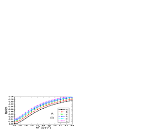
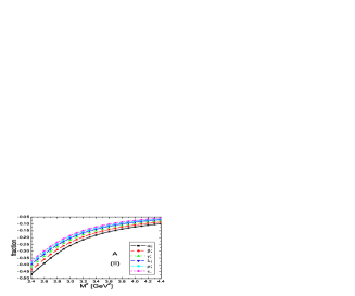
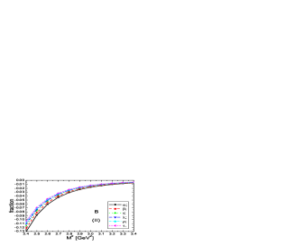
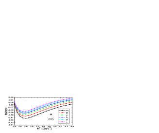
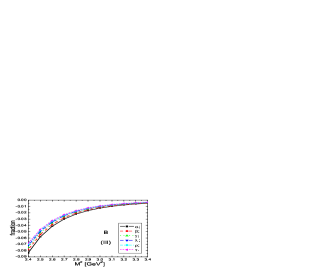
Figure 1: The contributions from different terms with variation of the Borel parameter $M^{2}$ in the operator product expansion for the $C\gamma_{5}-C\gamma_{\mu}\gamma_{5}$ type current operators. The $A$ and $B$ denote the contributions from the $\langle\bar{q}q\rangle^{2}+\langle\bar{q}q\rangle\langle\bar{q}g_{s}\sigma Gq\rangle$ term and the $\langle\bar{q}g_{s}\sigma Gq\rangle^{2}$ term, respectively. The (I), (II) and (III) denote the $c\bar{c}q\bar{q}$, $c\bar{c}q\bar{s}$ and $c\bar{c}s\bar{s}$ channels, respectively. The notations $\alpha$, $\beta$, $\gamma$, $\lambda$, $\rho$ and $\tau$ correspond to the threshold parameters $s_{0}=28\,\rm{GeV}^{2}$, $29\,\rm{GeV}^{2}$, $30\,\rm{GeV}^{2}$, $31\,\rm{GeV}^{2}$, $32\,\rm{GeV}^{2}$ and $33\,\rm{GeV}^{2}$, respectively.

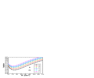
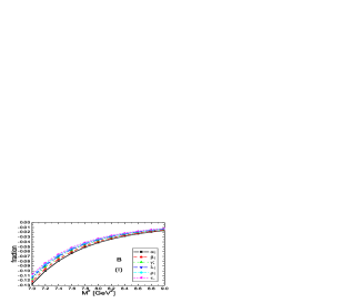
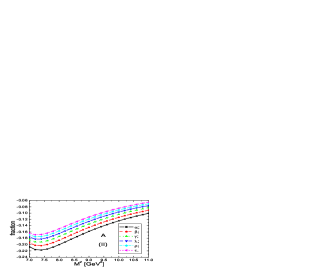
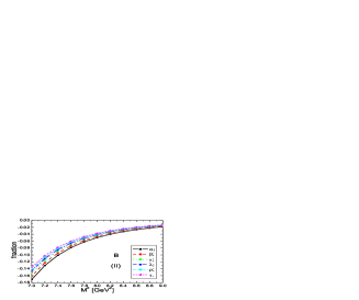
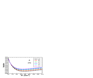
Figure 2: The contributions from different terms with variation of the Borel parameter $M^{2}$ in the operator product expansion for the $C\gamma_{5}-C\gamma_{\mu}\gamma_{5}$ type current operators. The $A$ and $B$ denote the contributions from the $\langle\bar{q}q\rangle^{2}+\langle\bar{q}q\rangle\langle\bar{q}g_{s}\sigma Gq\rangle$ term and the $\langle\bar{q}g_{s}\sigma Gq\rangle^{2}$ term, respectively. The (I), (II) and (III) denote the $b\bar{b}q\bar{q}$, $b\bar{b}q\bar{s}$ and $b\bar{b}s\bar{s}$ channels, respectively. The notations $\alpha$, $\beta$, $\gamma$, $\lambda$, $\rho$ and $\tau$ correspond to the threshold parameters $s_{0}=152\,\rm{GeV}^{2}$, $154\,\rm{GeV}^{2}$, $156\,\rm{GeV}^{2}$, $158\,\rm{GeV}^{2}$, $160\,\rm{GeV}^{2}$ and $162\,\rm{GeV}^{2}$, respectively.

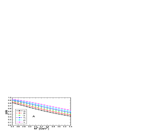
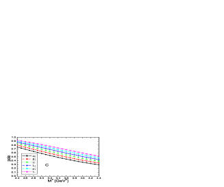
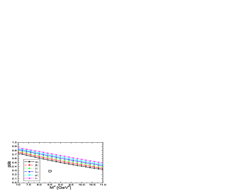
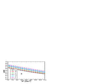
Figure 3: The contributions from the pole terms with variation of the Borel parameter $M^{2}$ for the $C\gamma_{5}-C\gamma_{\mu}\gamma_{5}$ type current opertors. The $A$, $B$, $C$, $D$, $E$ and $F$ denote the $c\bar{c}q\bar{q}$, $c\bar{c}q\bar{s}$, $c\bar{c}s\bar{s}$, $b\bar{b}q\bar{q}$, $b\bar{b}q\bar{s}$ and $b\bar{b}s\bar{s}$ channels, respectively. In the $c\bar{c}$ channels, the notations $\alpha$, $\beta$, $\gamma$, $\lambda$, $\rho$ and $\tau$ correspond to the threshold parameters $s_{0}=28\,\rm{GeV}^{2}$, $29\,\rm{GeV}^{2}$, $30\,\rm{GeV}^{2}$, $31\,\rm{GeV}^{2}$, $32\,\rm{GeV}^{2}$ and $33\,\rm{GeV}^{2}$ respectively ; while in the $b\bar{b}$ channels they correspond to the threshold parameters $s_{0}=152\,\rm{GeV}^{2}$, $154\,\rm{GeV}^{2}$, $156\,\rm{GeV}^{2}$, $158\,\rm{GeV}^{2}$, $160\,\rm{GeV}^{2}$ and $162\,\rm{GeV}^{2}$ respectively.

Taking into account all uncertainties of the input parameters, finally we obtain the values of the masses and pole resides of the vector hidden charm and bottom tetraquark states $Z$, which are shown in Figs.4-7 and Tables 1-2.

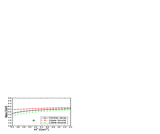
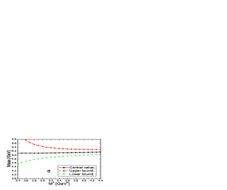
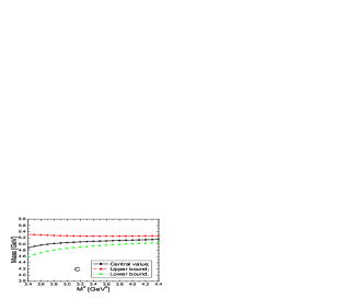
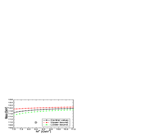
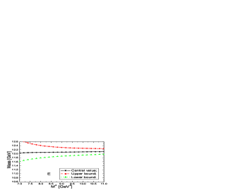
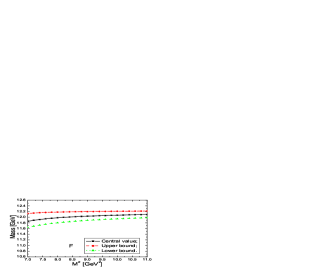
Figure 4: The masses of the vector tetraquark states with variation of the Borel parameter $M^{2}$ for the $C\gamma_{5}-C\gamma_{\mu}\gamma_{5}$ type current opertors. The $A$, $B$, $C$, $D$, $E$ and $F$ denote the $c\bar{c}q\bar{q}$, $c\bar{c}q\bar{s}$, $c\bar{c}s\bar{s}$, $b\bar{b}q\bar{q}$, $b\bar{b}q\bar{s}$ and $b\bar{b}s\bar{s}$ channels, respectively.

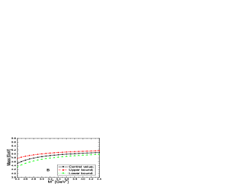
Figure 5: The masses of the vector tetraquark states with variation of the Borel parameter $M^{2}$ for the $C-C\gamma_{\mu}$ type current opertors. The $A$, $B$, $C$, $D$, $E$ and $F$ denote the $c\bar{c}q\bar{q}$, $c\bar{c}q\bar{s}$, $c\bar{c}s\bar{s}$, $b\bar{b}q\bar{q}$, $b\bar{b}q\bar{s}$ and $b\bar{b}s\bar{s}$ channels, respectively.

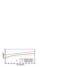
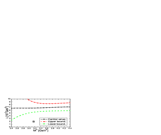
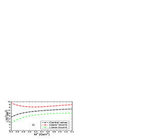
Figure 6: The pole residues of the vector tetraquark states with variation of the Borel parameter $M^{2}$ for the $C\gamma_{5}-C\gamma_{\mu}\gamma_{5}$ type current opertors. The $A$, $B$, $C$, $D$, $E$ and $F$ denote the $c\bar{c}q\bar{q}$, $c\bar{c}q\bar{s}$, $c\bar{c}s\bar{s}$, $b\bar{b}q\bar{q}$, $b\bar{b}q\bar{s}$ and $b\bar{b}s\bar{s}$ channels, respectively.

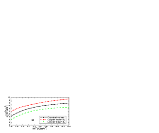
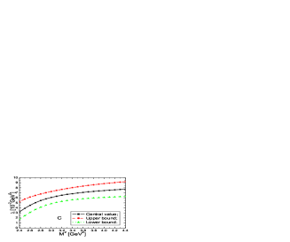
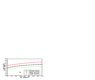
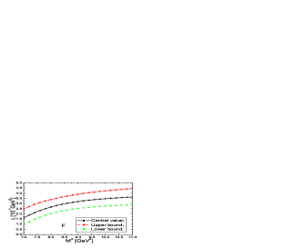
Figure 7: The pole residues of the vector tetraquark states with variation of the Borel parameter $M^{2}$ for the $C-C\gamma_{\mu}$ type current opertors. The $A$, $B$, $C$, $D$, $E$ and $F$ denote the $c\bar{c}q\bar{q}$, $c\bar{c}q\bar{s}$, $c\bar{c}s\bar{s}$, $b\bar{b}q\bar{q}$, $b\bar{b}q\bar{s}$ and $b\bar{b}s\bar{s}$ channels, respectively.

tetraquark states	$C\gamma_{5}-C\gamma_{\mu}\gamma_{5}$	$C-C\gamma_{\mu}$
$c\bar{c}q\bar{q}$	$4.97\pm 0.14$	$4.95\pm 0.14$
$c\bar{c}q\bar{s}$	$5.12\pm 0.20$	$5.00\pm 0.15$
$c\bar{c}s\bar{s}$	$5.10\pm 0.17$	$5.05\pm 0.15$
$b\bar{b}q\bar{q}$	$11.90\pm 0.14$	$11.90\pm 0.14$
$b\bar{b}q\bar{s}$	$12.08\pm 0.23$	$11.89\pm 0.17$
$b\bar{b}s\bar{s}$	$12.04\pm 0.17$	$11.95\pm 0.16$

Table 1: The masses (in unit of GeV) of the vector tetraquark states.

tetraquark states	$C\gamma_{5}-C\gamma_{\mu}\gamma_{5}$	$C-C\gamma_{\mu}$
$c\bar{c}q\bar{q}$	$6.3\pm 1.4$	$6.5\pm 1.4$
$c\bar{c}q\bar{s}$	$6.9\pm 1.4$	$7.2\pm 1.7$
$c\bar{c}s\bar{s}$	$7.1\pm 1.5$	$7.1\pm 1.6$
$b\bar{b}q\bar{q}$	$3.0\pm 0.7$	$3.1\pm 0.7$
$b\bar{b}q\bar{s}$	$3.4\pm 0.8$	$3.3\pm 0.8$
$b\bar{b}s\bar{s}$	$3.4\pm 0.8$	$3.2\pm 0.8$

Table 2: The pole residues (in unit of $10^{-2}\,\rm{GeV}^{5}$ and $10^{-1}\,\rm{GeV}^{5}$ for the $c\bar{c}$ and $b\bar{b}$ channels respectively) of the vector tetraquark states.

From Table 1, we can see that the $SU(3)$ breaking effects for the masses of the hidden charm and bottom tetraquark states are buried in the uncertainties. The central values of the vector tetraquark state $c\bar{c}q\bar{q}$ is slightly below the ones $M_{Z}=(5.12\pm 0.15)\,\rm{GeV}$ and $M_{Z}=(5.16\pm 0.16)\,\rm{GeV}$ obtained in Ref.[9], about $0.15\,\rm{GeV}$. In Ref.[9], the contributions from the terms $\langle\bar{q}q\rangle\langle\bar{q}g_{s}\sigma Gq\rangle$ and $\langle\bar{q}g_{s}\sigma Gq\rangle^{2}$ are neglected.

We calculate the mass spectrum of the vector hidden charm and bottom tetraquark states by imposing the two criteria of the QCD sum rules. In fact, we usually consult the experimental data in choosing the Borel parameter $M^{2}$ and the threshold parameter $s_{0}$. There lack experimental data for the phenomenological hadronic spectral densities of the tetraquark states, the present predictions can’t be confronted with the experimental data.

In Refs.[27, 28, 29, 30, 31], Maiani et al take the diquarks as the basic constituents, examine the rich spectrum of the diquark-antidiquark states from the constituent diquark masses and the spin-spin interactions, and try to accommodate some of the newly observed charmonium-like resonances not fitting a pure $c\bar{c}$ assignment. The predictions depend heavily on the assumption that the light scalar mesons $a_{0}(980)$ and $f_{0}(980)$ are tetraquark states, the basic parameters (constituent diquark masses) are estimated thereafter. In the conventional quark models, the constituent quark masses are taken as the basic input parameters, and fitted to reproduce the mass spectra of the conventional mesons and baryons. However, the present experimental knowledge about the phenomenological hadronic spectral densities of the multiquark states is rather vague, even existence of the multiquark states is not confirmed with confidence, and no knowledge about either there are high resonances or not. The predicted constituent diquark masses can not be confronted with the experimental data.

The LHCb is a dedicated $b$ and $c$-physics precision experiment at the LHC (large hadron collider). The LHC will be the world’s most copious source of the $b$ hadrons, and a complete spectrum of the $b$ hadrons will be available through gluon fusion. In proton-proton collisions at $\sqrt{s}=14\,\rm{TeV}$ , the $b\bar{b}$ cross section is expected to be $\sim 500\mu b$ producing $10^{12}$ $b\bar{b}$ pairs in a standard year of running at the LHCb operational luminosity of $2\times 10^{32}\rm{cm}^{-2}\rm{sec}^{-1}$ [14]. The vector tetraquark states predicted in the present work may be observed at the LHCb, if they exist indeed. We can search for the vector hidden charm tetraquark states in the $D\bar{D}$, $D\bar{D^{*}}$, $D^{*}\bar{D^{*}}$, $D_{s}\bar{D_{s}}$, $D_{s}\bar{D^{*}_{s}}$, $D_{s}^{*}\bar{D_{s}^{*}}$, $J/\psi\rho$, $J/\psi\phi$, $J/\psi\omega$, $J/\psi\pi$, $J/\psi f_{0}(980)$, $J/\psi K$, $\eta_{c}\pi$, $\eta_{c}\eta$, $\cdots$ invariant mass distributions and search for the vector hidden bottom tetraquark states in the $B\bar{B}$, $B\bar{B^{*}}$, $B^{*}\bar{B^{*}}$, $B_{s}\bar{B_{s}}$, $B_{s}\bar{B_{s}^{*}}$, $B_{s}^{*}\bar{B_{s}^{*}}$, $\Upsilon\rho$, $\Upsilon\phi$, $\Upsilon\omega$, $\Upsilon\pi$, $\Upsilon K$, $\Upsilon f_{0}(980)$, $\eta_{b}\pi$, $\eta_{b}\eta$, $\cdots$ invariant mass distributions.

4 Conclusion

In this article, we study the mass spectrum of the vector hidden charm and bottom tetraquark states with the QCD sum rules. The mass spectrum are calculated by imposing the two criteria (pole dominance and convergence of the operator product expansion) of the QCD sum rules. As there lack experimental data for the phenomenological hadronic spectral densities of the tetraquark states, the present predictions can’t be confronted with the experimental data. We can search for the vector hidden charm and bottom tetraquark states at the LHCb or the Fermi-lab Tevatron.

Appendix

The spectral densities at the level of the quark-gluon degrees of freedom:

$$\rho^{\pm}_{q\bar{q}}(s) = \frac{1}{3072\pi^{6}}\int_{\alpha_{min}}^{\alpha_{max}}d\alpha\int_{\beta_{min}}^{1-\alpha}d\beta\alpha\beta(1-\alpha-\beta)^{3}(s-\widetilde{m}^{2}_{Q})^{2}(35s^{2}-26s\widetilde{m}^{2}_{Q}+3\widetilde{m}^{4}_{Q})$$ (10)

$$\pm\frac{m_{Q}\langle\bar{q}q\rangle}{32\pi^{4}}\int_{\alpha_{min}}^{\alpha_{max}}d\alpha\int_{\beta_{min}}^{1-\alpha}d\beta(1-\alpha-\beta)(s-\widetilde{m}^{2}_{Q})\left[(4\beta-3\alpha)s+(\alpha-2\beta)\widetilde{m}^{2}_{Q}\right]$$

$$\pm\frac{m_{Q}\langle\bar{q}g_{s}\sigma Gq\rangle}{64\pi^{4}}\int_{\alpha_{min}}^{\alpha_{max}}d\alpha\int_{\beta_{min}}^{1-\alpha}d\beta\left[(2\alpha-3\beta)s-(\alpha-2\beta)\widetilde{m}^{2}_{Q})\right]$$

$$-\frac{m_{Q}^{2}\langle\bar{q}q\rangle^{2}}{12\pi^{2}}\int_{\alpha_{mix}}^{\alpha_{max}}d\alpha+\frac{m_{Q}^{2}\langle\bar{q}q\rangle\langle\bar{q}g_{s}\sigma Gq\rangle}{24\pi^{2}}\int_{\alpha_{mix}}^{\alpha_{max}}d\alpha\left[1+\frac{s}{M^{2}}\right]\delta(s-\widetilde{\widetilde{m}}_{Q}^{2})$$

$$-\frac{m_{Q}^{2}\langle\bar{q}g_{s}\sigma Gq\rangle^{2}}{192\pi^{2}M^{6}}\int_{\alpha_{mix}}^{\alpha_{max}}d\alpha\widetilde{\widetilde{m}}_{Q}^{4}\delta(s-\widetilde{\widetilde{m}}_{Q}^{2})\,,$$

$$\rho^{\pm}_{q\bar{s}}(s) = \frac{1}{3072\pi^{6}}\int_{\alpha_{min}}^{\alpha_{max}}d\alpha\int_{\beta_{min}}^{1-\alpha}d\beta\alpha\beta(1-\alpha-\beta)^{3}(s-\widetilde{m}^{2}_{Q})^{2}(35s^{2}-26s\widetilde{m}^{2}_{Q}+3\widetilde{m}^{4}_{Q})$$ (11)

$$\mp\frac{m_{s}m_{Q}}{256\pi^{6}}\int_{\alpha_{min}}^{\alpha_{max}}d\alpha\int_{\beta_{min}}^{1-\alpha}d\beta\beta(1-\alpha-\beta)^{2}(s-\widetilde{m}^{2}_{Q})^{2}(5s-2\widetilde{m}^{2}_{Q})$$

$$+\frac{m_{s}\langle\bar{s}s\rangle}{64\pi^{4}}\int_{\alpha_{min}}^{\alpha_{max}}d\alpha\int_{\beta_{min}}^{1-\alpha}d\beta\alpha\beta(1-\alpha-\beta)(15s^{2}-16s\widetilde{m}^{2}_{Q}+3\widetilde{m}^{4}_{Q})$$

$$\pm\frac{m_{Q}\langle\bar{q}q\rangle}{32\pi^{4}}\int_{\alpha_{min}}^{\alpha_{max}}d\alpha\int_{\beta_{min}}^{1-\alpha}d\beta\alpha(1-\alpha-\beta)(s-\widetilde{m}^{2}_{Q})(\widetilde{m}^{2}_{Q}-3s)$$

$$\mp\frac{m_{Q}\langle\bar{s}s\rangle}{16\pi^{4}}\int_{\alpha_{min}}^{\alpha_{max}}d\alpha\int_{\beta_{min}}^{1-\alpha}d\beta\beta(1-\alpha-\beta)(s-\widetilde{m}^{2}_{Q})(\widetilde{m}^{2}_{Q}-2s)$$

$$\pm\frac{m_{Q}\langle\bar{q}g_{s}\sigma Gq\rangle}{64\pi^{4}}\int_{\alpha_{min}}^{\alpha_{max}}d\alpha\int_{\beta_{min}}^{1-\alpha}d\beta\alpha(2s-\widetilde{m}^{2}_{Q})$$

$$\mp\frac{m_{Q}\langle\bar{s}g_{s}\sigma Gs\rangle}{64\pi^{4}}\int_{\alpha_{min}}^{\alpha_{max}}d\alpha\int_{\beta_{min}}^{1-\alpha}d\beta\beta(3s-2\widetilde{m}^{2}_{Q})$$

$$-\frac{m_{s}\langle\bar{s}g_{s}\sigma Gs\rangle}{192\pi^{4}}\int_{\alpha_{min}}^{\alpha_{max}}d\alpha\int_{\beta_{min}}^{1-\alpha}d\beta\alpha\beta\left[8s-3\widetilde{m}^{2}_{Q}+s^{2}\delta(s-\widetilde{m}^{2}_{Q})\right]$$

$$+\frac{m_{s}m_{Q}^{2}\langle\bar{q}q\rangle}{16\pi^{4}}\int_{\alpha_{min}}^{\alpha_{max}}d\alpha\int_{\beta_{min}}^{1-\alpha}d\beta(s-\widetilde{m}^{2}_{Q})$$

$$-\frac{m_{Q}^{2}\langle\bar{q}q\rangle\langle\bar{s}s\rangle}{12\pi^{2}}\int_{\alpha_{mix}}^{\alpha_{max}}d\alpha-\frac{m_{s}m_{Q}^{2}\langle\bar{q}g_{s}\sigma Gq\rangle}{64\pi^{4}}\int_{\alpha_{mix}}^{\alpha_{max}}d\alpha$$

$$\mp\frac{m_{s}m_{Q}\langle\bar{q}q\rangle\langle\bar{s}s\rangle}{24\pi^{2}}\int_{\alpha_{mix}}^{\alpha_{max}}d\alpha\alpha\left[2+s\delta(s-\widetilde{\widetilde{m}}^{2}_{Q})\right]$$

$$+\frac{m_{Q}^{2}\left[\langle\bar{q}q\rangle\langle\bar{s}g_{s}\sigma Gs\rangle+\langle\bar{s}s\rangle\langle\bar{q}g_{s}\sigma Gq\rangle\right]}{48\pi^{2}}\int_{\alpha_{mix}}^{\alpha_{max}}d\alpha\left[1+\frac{s}{M^{2}}\right]\delta(s-\widetilde{\widetilde{m}}_{Q}^{2})$$

$$\pm\frac{m_{s}m_{Q}\left[2\langle\bar{q}q\rangle\langle\bar{s}g_{s}\sigma Gs\rangle+3\langle\bar{s}s\rangle\langle\bar{q}g_{s}\sigma Gq\rangle\right]}{288\pi^{2}M^{2}}\int_{\alpha_{mix}}^{\alpha_{max}}d\alpha\alpha\left[s-\frac{s^{2}}{M^{2}}\right]\delta(s-\widetilde{\widetilde{m}}_{Q}^{2})$$

$$-\frac{m_{Q}^{2}\langle\bar{q}g_{s}\sigma Gq\rangle\langle\bar{s}g_{s}\sigma Gs\rangle}{192\pi^{2}M^{6}}\int_{\alpha_{mix}}^{\alpha_{max}}d\alpha\widetilde{\widetilde{m}}_{Q}^{4}\delta(s-\widetilde{\widetilde{m}}_{Q}^{2})\,,$$

$$\rho^{\pm}_{s\bar{s}}(s) = \frac{1}{3072\pi^{6}}\int_{\alpha_{min}}^{\alpha_{max}}d\alpha\int_{\beta_{min}}^{1-\alpha}d\beta\alpha\beta(1-\alpha-\beta)^{3}(s-\widetilde{m}^{2}_{Q})^{2}(35s^{2}-26s\widetilde{m}^{2}_{Q}+3\widetilde{m}^{4}_{Q})$$ (12)

$$\pm\frac{m_{s}m_{Q}}{256\pi^{6}}\int_{\alpha_{min}}^{\alpha_{max}}d\alpha\int_{\beta_{min}}^{1-\alpha}d\beta(1-\alpha-\beta)^{2}(s-\widetilde{m}^{2}_{Q})^{2}\left[(4\alpha-5\beta)s-(\alpha-2\beta)\widetilde{m}^{2}_{Q}\right]$$

$$+\frac{m_{s}\langle\bar{s}s\rangle}{32\pi^{4}}\int_{\alpha_{min}}^{\alpha_{max}}d\alpha\int_{\beta_{min}}^{1-\alpha}d\beta\alpha\beta(1-\alpha-\beta)(15s^{2}-16s\widetilde{m}^{2}_{Q}+3\widetilde{m}^{4}_{Q})$$

$$\pm\frac{m_{Q}\langle\bar{s}s\rangle}{16\pi^{4}}\int_{\alpha_{min}}^{\alpha_{max}}d\alpha\int_{\beta_{min}}^{1-\alpha}d\beta(1-\alpha-\beta)(s-\widetilde{m}^{2}_{Q})\left[(4\beta-3\alpha)s+(\alpha-2\beta)\widetilde{m}^{2}_{Q}\right]$$

$$\pm\frac{m_{Q}\langle\bar{s}g_{s}\sigma Gs\rangle}{64\pi^{4}}\int_{\alpha_{min}}^{\alpha_{max}}d\alpha\int_{\beta_{min}}^{1-\alpha}d\beta\left[(2\alpha-3\beta)s-(\alpha-2\beta)\widetilde{m}^{2}_{Q}\right]$$

$$-\frac{m_{s}\langle\bar{s}g_{s}\sigma Gs\rangle}{96\pi^{4}}\int_{\alpha_{min}}^{\alpha_{max}}d\alpha\int_{\beta_{min}}^{1-\alpha}d\beta\alpha\beta\left[8s-3\widetilde{m}^{2}_{Q}+s^{2}\delta(s-\widetilde{m}^{2}_{Q})\right]$$

$$+\frac{m_{s}m_{Q}^{2}\langle\bar{s}s\rangle}{8\pi^{4}}\int_{\alpha_{min}}^{\alpha_{max}}d\alpha\int_{\beta_{min}}^{1-\alpha}d\beta(s-\widetilde{m}^{2}_{Q})$$

$$-\frac{m_{Q}^{2}\langle\bar{s}s\rangle^{2}}{12\pi^{2}}\int_{\alpha_{mix}}^{\alpha_{max}}d\alpha-\frac{m_{s}m_{Q}^{2}\langle\bar{s}g_{s}\sigma Gs\rangle}{32\pi^{4}}\int_{\alpha_{mix}}^{\alpha_{max}}d\alpha$$

$$+\frac{m_{Q}^{2}\langle\bar{s}s\rangle\langle\bar{s}g_{s}\sigma Gs\rangle}{24\pi^{2}}\int_{\alpha_{mix}}^{\alpha_{max}}d\alpha\left[1+\frac{s}{M^{2}}\right]\delta(s-\widetilde{\widetilde{m}}_{Q}^{2})$$

$$\pm\frac{5m_{s}m_{Q}\langle\bar{s}s\rangle\langle\bar{s}g_{s}\sigma Gs\rangle}{288\pi^{2}M^{2}}\int_{\alpha_{mix}}^{\alpha_{max}}d\alpha\alpha\left[s-\frac{s^{2}}{M^{2}}\right]\delta(s-\widetilde{\widetilde{m}}_{Q}^{2})$$

$$\mp\frac{5m_{s}m_{Q}\langle\bar{s}s\rangle\langle\bar{s}g_{s}\sigma Gs\rangle}{144\pi^{2}}\int_{\alpha_{mix}}^{\alpha_{max}}d\alpha(1-\alpha)\left[1+\frac{s}{M^{2}}+\frac{s^{2}}{2M^{4}}\right]\delta(s-\widetilde{\widetilde{m}}_{Q}^{2})$$

$$-\frac{m_{Q}^{2}\langle\bar{s}g_{s}\sigma Gs\rangle^{2}}{192\pi^{2}M^{6}}\int_{\alpha_{mix}}^{\alpha_{max}}d\alpha\widetilde{\widetilde{m}}_{Q}^{4}\delta(s-\widetilde{\widetilde{m}}_{Q}^{2})\,,$$

References

[1] E. S. Swanson, Phys. Rept. 429 (2006) 243.
[2] E. Klempt and A. Zaitsev, Phys. Rept. 454 (2007) 1.
[3] M. B. Voloshin, Prog. Part. Nucl. Phys. 61 (2008) 455.
[4] S. Godfrey and S. L. Olsen, Ann. Rev. Nucl. Part. Sci. 58 (2008) 51.
[5] S. L. Olsen, arXiv:0901.2371.
[6] S. K. Choi et al, Phys. Rev. Lett. 100 (2008) 142001.
[7] B. Aubert et al, arXiv:0811.0564.
[8] R. Mizuk et al, Phys. Rev. D78 (2008) 072004.
[9] Z. G. Wang, Eur. Phys. J. C59 (2009) 675.
[10] Z. G. Wang, arXiv:0807.4592.
[11] Z. G. Wang, arXiv:0902.2062.
[12] M. A. Shifman, A. I. Vainshtein and V. I. Zakharov,
Nucl. Phys. B147 (1979) 385, 448.
[13] L. J. Reinders, H. Rubinstein and S. Yazaki, Phys. Rept. 127 (1985) 1.
[14] G. Kane and A. Pierce, ”Perspectives On LHC Physics”,
World Scientific Publishing Company, 2008.
[15] R. L. Jaffe and F. Wilczek, Phys. Rev. Lett. 91 (2003) 232003.
[16] R. L. Jaffe, Phys. Rept. 409 (2005) 1.
[17] A. De Rujula, H. Georgi and S. L. Glashow, Phys. Rev. D12
(1975) 147.
[18] T. DeGrand, R. L. Jaffe, K. Johnson and J. E. Kiskis,
Phys. Rev. D12 (1975) 2060.
[19] Z. G. Wang, Nucl. Phys. A791 (2007) 106.
[20] Z. G. Wang, W. M. Yang and S. L. Wan, J. Phys. G31 (2005) 971.
[21] Z. G. Wang, arXiv:0903.5200.
[22] N. Kodama, M. Oka and T. Hatsuda, Nucl. Phys. A580 (1994) 445.
[23] B. L. Ioffe, Prog. Part. Nucl. Phys. 56 (2006)
232.
[24] A. Khodjamirian and R. Ruckl, Adv. Ser. Direct. High Energy Phys. 15 (1998) 345.
[25] C. Amsler et al, Phys. Lett. B667 (2008) 1.
[26] Z. G. Wang, Chin. Phys. C32 (2008) 797.
[27] L. Maiani, F. Piccinini, A. D. Polosa and V. Riquer, Phys. Rev. Lett. 93 (2004) 212002.
[28] L. Maiani, F. Piccinini, A. D. Polosa and V. Riquer, Phys. Rev. D71 (2005) 014028.
[29] L. Maiani, F. Piccinini, A. D. Polosa and V. Riquer, Phys. Rev. D72 (2005) 031502.
[30] L. Maiani, A. D. Polosa and V. Riquer, New J. Phys. 10 (2008) 073004.
[31] N. V. Drenska, R. Faccini and A. D. Polosa, arXiv:0902.2803.