Rabinowitz Floer homology and symplectic homology

Abstract.

The first two authors have recently defined Rabinowitz-Floer homology groups $RFH_{*}(M,W)$ associated to an exact embedding of a contact manifold $(M,\xi)$ into a symplectic manifold $(W,\omega)$. These depend only on the bounded component $V$ of $W\setminus M$. We construct a long exact sequence in which symplectic cohomology of $V$ maps to symplectic homology of $V$, which in turn maps to Rabinowitz-Floer homology $RFH_{*}(M,W)$, which then maps to symplectic cohomology of $V$. We compute $RFH_{*}(ST^{*}L,T^{*}L)$, where $ST^{*}L$ is the unit cosphere bundle of a closed manifold $L$. As an application, we prove that the image of an exact contact embedding of $ST^{*}L$ (endowed with the standard contact structure) cannot be displaced away from itself by a Hamiltonian isotopy, provided $\dim\,L\geq 4$ and the embedding induces an injection on $\pi_{1}$. In particular, $ST^{*}L$ does not admit an exact contact embedding into a subcritical Stein manifold if $L$ is simply connected. We also prove that Weinstein’s conjecture holds in symplectic manifolds which admit exact displaceable codimension $0$ embeddings.

1. Introduction

Let $(W,\lambda)$ be a complete convex exact symplectic manifold, with symplectic form $\omega=d\lambda$ (see Section 3 for the precise definition). An embedding $\iota:M\hookrightarrow W$ of a contact manifold $(M,\xi)$ is called exact contact embedding if there exists a 1-form $\alpha$ on $M$ such that such that $\ker\alpha=\xi$ and $\alpha-\lambda|_{M}$ is exact. We identify $M$ with its image $\iota(M)$. We assume that $W\setminus M$ consists of two connected components and denote the bounded component of $W\setminus M$ by $V$. One can classically [25] associate to such an exact contact embedding the symplectic (co)homology groups $SH_{*}(V)$ and $SH^{*}(V)$. We refer to Section 2 for the definition and basic properties, and to [22] for a recent survey.

The first two authors have recently defined for such an exact contact embedding Floer homology groups $RFH_{*}(M,W)$ for the Rabinowitz action functional [9]. We refer to Section 3 for a recap of the definition and of some useful properties. We will show in particular that these groups do not depend on $W$, but only on $V$ (the same holds for $SH_{*}(V)$ and $SH^{*}(V)$). We shall use in this paper the notation $RFH_{*}(V)$ and call them Rabinowitz Floer homology groups.

Remark 1.1.

All (co)homology groups are taken with field coefficients. Without any further hypotheses on the first Chern class $c_{1}(V)$ of the tangent bundle, the symplectic (co)homology and Rabinowitz Floer homology groups are ${\mathbb{Z}}_{2}$-graded. If $c_{1}(V)=0$ they are ${\mathbb{Z}}$-graded, and if $c_{1}(V)$ vanishes on $\pi_{2}(V)$ the part constructed from contractible loops is ${\mathbb{Z}}$-graded. This ${\mathbb{Z}}$-grading on Rabinowitz Floer homology differs from the one in [9] (which takes values in $\frac{1}{2}+{\mathbb{Z}}$) by a shift of $1/2$ (see Remark 3.2).

Our purpose is to relate these two constructions. The relevant object is a new version of symplectic homology, denoted $\check{SH}_{*}(V)$, associated to “$\bigvee$-shaped” Hamiltonians like the one in Figure 1 on page 1 below. This version of symplectic homology is related to the usual ones via the long exact sequence in the next theorem.

Theorem 1.2.

There is a long exact sequence

(1)

The long exact sequence (1) can be seen as measuring the defect from being an isomorphism of the canonical map $SH^{-*}(V)\to SH_{*}(V)$, which we define in Section 2.7. An interesting fact is that we have a very precise description of this map. To state it, let us recall that there are canonical morphisms induced by truncation of the range of the action $H_{*+n}(V,\partial V)\stackrel{{\scriptstyle c_{*}}}{{\longrightarrow}}SH_{*}(V)$ and $SH^{*}(V)\stackrel{{\scriptstyle c^{*}}}{{\longrightarrow}}H^{*+n}(V,\partial V)$ (see [25] or Lemma 2.1 below).

Proposition 1.3.

The map $SH^{-*}(V)\to SH_{*}(V)$ fits into a commutative diagram

(2)

in which the bottom arrow is the composition of the map induced by the inclusion $V\hookrightarrow(V,\partial V)$ with the Poincaré duality isomorphism

$$H^{-*+n}(V,\partial V)\stackrel{{\scriptstyle PD}}{{\longrightarrow}}H_{*+n}(V)\stackrel{{\scriptstyle incl_{*}}}{{\longrightarrow}}H_{*+n}(V,\partial V).$$

We also define in Section 2.7 truncated versions $\check{SH}_{*}^{\geq 0}(V)$ and $\check{SH}_{*}^{\leq 0}(V)$ of the symplectic homology groups $\check{SH}_{*}(V)$.

Proposition 1.4.

There are commuting diagrams of long exact sequences as below, where $PD$ denotes Poincaré duality and the top exact sequence is the (co)homological long exact sequence of the pair $(V,M)$:

and

The main result of this paper is the following.

Theorem 1.5.

We have an isomorphism

$$RFH_{*}(V)\simeq\check{SH}_{*}(V).$$

Theorem 1.5 is proved in Section 6. It follows that the Rabinowitz Floer homology groups fit into a long exact sequence

(3)

We also recall the following vanishing result for Rabinowitz Floer homology from [9].

Theorem 1.6 ([9, Theorem 1.2]).

If $M={\partial}V$ is Hamiltonianly displaceable in $W$, then

$$RFH_{*}(V)=0.$$

To state the next corollary, we recall that the symplectic (co)homology and Rabinowitz Floer homology groups decompose as direct sums

$$SH_{*}(V)=\oplus_{c}SH_{*}^{c}(V),\ \ SH^{*}(V)=\oplus_{c}SH^{*}_{c}(V),\ \ RFH_{*}(V)=\oplus_{c}RFH_{*}^{c}(V)$$

indexed over free homotopy classes of loops in $V$. We denote the free homotopy class of the constant loops by $c=0$.

Corollary 1.7.

Assume $M=\partial V$ is Hamiltonianly displaceable in $W$.

• For $c\neq 0$ we have

  $$SH_{*}^{c}(V)=0,\quad SH^{*}_{c}(V)=0.$$

• Suppose that $c_{1}(W)|_{\pi_{2}(W)}=0$. Then for $c=0$ we have

  (4) $$SH_{*}^{c=0}(V)=0,\quad SH^{*}_{c=0}(V)=0$$

  if $*\geq n$ or $*\leq-n$. Moreover, if $V$ is Stein then (4) holds for $*\neq 0$, and if $V$ is Stein subcritical then (4) holds for all $*\in{\mathbb{Z}}$.

Proof.

The long exact sequence (3) splits into a direct sum of long exact sequences, indexed over free homotopy classes of loops in $V$. The assumption that $M$ is Hamiltonianly displaceable implies $RFH_{*}(V)=0$, hence the map $SH^{-*}_{c}(V)\to SH_{*}^{c}(V)$ is an isomorphism for any $c$.

We now use the commutative diagram in Proposition 1.3 and the fact that the canonical map $c_{*}:H_{*+n}(V,{\partial}V)\to SH_{*}(V)$ takes values into the direct summand $SH_{*}^{c=0}(V)$, and similarly, the map $c^{*}:SH^{*}(V)\to H^{*+n}(V,{\partial}V)$ factors through $SH^{*}_{c=0}(V)$ (see Lemma 2.1 and Lemma 2.4 below).

Let us assume $c\neq 0$. Then the above discussion shows that the map $SH^{-*}_{c}(V)\to SH_{*}^{c}(V)$ is at the same time an isomorphism and vanishes. This implies the conclusion.

Let us now assume $c=0$ and $c_{1}(W)|_{\pi_{2}(W)}=0$, so that all homology groups are ${\mathbb{Z}}$-graded. By Proposition 1.3, the map $SH^{-*}_{c=0}(V)\to SH_{*}^{c=0}(V)$ is the composition

$$SH^{-*}_{c=0}(V)\to H^{-*+n}(V,{\partial}V)\simeq H_{*+n}(V)\to H_{*+n}(V,{\partial}V)\to SH_{*}^{c=0}(V),$$

and therefore vanishes if $H_{*+n}(V)=0$ or $H_{*+n}(V,{\partial}V)\cong H^{n-*}(V)=0$. This is always the case if $*\geq n$ or $*\leq-n$. If $V$ is Stein, this holds if $*\neq 0$, and if $V$ is Stein subcritical, this holds for all $*\in{\mathbb{Z}}$. The conclusion follows. ∎

Corollary 1.8 ([7]).

If $V$ is Stein subcritical and $c_{1}(V)|_{\pi_{2}(V)}=0$, then $SH_{*}(V)=0$.

Proof.

Any compact set in a subcritical Stein manifold is Hamiltonianly displaceable [3]. Thus $V$ is displaceable in $\widehat{V}$, and therefore $SH_{*}(V)=0$ by Corollary 1.7. ∎

Remark. The original proof of Corollary 1.8 in [7] uses a handle decomposition for $W$. The proof given above only uses the fact that the subcritical skeleton can be displaced from itself [3]. On the other hand, the proof given above uses the grading in an essential way and hence only works under the hypothesis $c_{1}(V)|_{\pi_{2}(V)}=0$, whereas the original proof does not need this assumption.

Corollary 1.9 (Weinstein conjecture in displaceable manifolds).

Assume that $V$ is Hamiltonianly displaceable in $W$ and $c_{1}(W)|_{\pi_{2}(W)}=0$. Then any hypersurface of contact type $\Sigma\subset V$ carries a closed characteristic.

Proof.

This follows from the fact that $SH^{n}_{c=0}(V)=0$, as proved in Corollary 1.7 above. In particular the canonical map $SH^{n}_{c=0}(V)\to H^{2n}(V,\partial V)$ vanishes, and thus $V$ satisfies the Strong Algebraic Weinstein Conjecture in the sense of Viterbo [25]. The conclusion is then a consequence of the Main Theorem in [25] (see also [15, Theorem 4.10] for details). ∎

We now turn to the computation of the Rabinowitz Floer homology groups for cotangent bundles. Let $L$ be a connected closed Riemannian manifold, and let $DT^{*}L\subset T^{*}L$ be the unit disc bundle with its canonical symplectic structure. Note that $c_{1}(T^{*}L)=0$, so its symplectic (co)homology and Rabinowitz Floer homology groups are ${\mathbb{Z}}$-graded. Given a free homotopy class $c$ of loops in $L$, we denote by $\Lambda^{c}L$ the corresponding connected component of the free loop space of $L$. Rabinowitz Floer homology $RFH_{*}(DT^{*}L)$ decomposes as a direct sum of homology groups $RFH_{*}^{c}(DT^{*}L)$ which only take into account loops in the class $c$. We denote the free homotopy class of the constant loops by $c=0$. We denote the Euler number of the cotangent bundle $T^{*}L\to L$ by $e(T^{*}L)$ (if $L$ is non-orientable we work with ${\mathbb{Z}}/2$-coefficients).

Theorem 1.10.

In degrees $*\neq 0,1$ the Rabinowitz Floer homology of $DT^{*}L$ is given by

$$RFH_{*}(DT^{*}L)=\left\{\begin{array}[]{rl}H_{*}(\Lambda L),&*>1,\\ H^{-*+1}(\Lambda L),&*<0.\end{array}\right.$$

In degree $0$ we have

$$RFH_{0}^{c}(DT^{*}L)=\left\{\begin{array}[]{ll}H_{0}(\Lambda^{c}L)\oplus H^{1}(\Lambda^{c}L),&if\ c\neq 0,\\ H_{0}(\Lambda^{0}L)\oplus H^{1}(\Lambda^{0}L),&if\ c=0\ and\ e(T^{*}L)=0,\\ H^{1}(\Lambda^{0}L),&if\ c=0\ and\ e(T^{*}L)\neq 0.\end{array}\right.$$

In degree $1$ we have

$$RFH_{1}^{c}(DT^{*}L)=\left\{\begin{array}[]{ll}H_{1}(\Lambda^{c}L)\oplus H^{0}(\Lambda^{c}L),&if\ c\neq 0,\\ H_{1}(\Lambda^{0}L)\oplus H^{0}(\Lambda^{0}L),&if\ c=0\ and\ e(T^{*}L)=0,\\ H_{1}(\Lambda^{0}L),&if\ c=0\ and\ e(T^{*}L)\neq 0.\end{array}\right.$$

The proof is based on the isomorphisms

(5) $$SH_{*}^{c}(DT^{*}L)\simeq H_{*}(\Lambda^{c}L),\qquad SH^{*}_{c}(DT^{*}L)\simeq H^{*}(\Lambda^{c}L),$$

proved in [26, 1, 19]. In particular $SH_{0}^{c}(DT^{*}L)$ and $SH^{0}_{c}(DT^{*}L)$ are isomorphic to the ground field. We also need the following Lemma.

Lemma 1.11.

The map $SH^{0}_{c}(DT^{*}L)\to SH_{0}^{c}(DT^{*}L)$ in the exact sequence of Theorem 1.2 vanishes if $c\neq 0$, and is multiplication by the Euler number $e(T^{*}L)$ if $c=0$.

Proof.

That the map $SH^{0}_{c}(DT^{*}L)\to SH_{0}^{c}(DT^{*}L)$ vanishes if $c\neq 0$ follows from the same argument as in Corollary 1.7.

Let us focus on the map $SH^{0}_{c=0}(DT^{*}L)\to SH_{0}^{c=0}(DT^{*}L)$. Modulo the isomorphisms with $H_{0}(\Lambda^{0}L)$, $H^{0}(\Lambda^{0}L)$, the commutative diagram (2) becomes

The vertical map on the left factors as

$$H^{0}(\Lambda^{0}L)\stackrel{{\scriptstyle incl^{*}}}{{\longrightarrow}}H^{0}(L)\stackrel{{\scriptstyle\simeq}}{{\longrightarrow}}H^{0}(DT^{*}L)\stackrel{{\scriptstyle\cup\tau}}{{\longrightarrow}}H^{n}(DT^{*}L,ST^{*}L),$$

where $incl^{*}$ is the isomorphism induced by the inclusion of constant loops, and $\cup\tau$ is the Thom isomorphism given by cup-product with the Thom class $\tau\in H^{n}(DT^{*}L,ST^{*}L)$ (see [25]). The vertical map on the right factors as

$$H_{n}(DT^{*}L,ST^{*}L)\stackrel{{\scriptstyle\cap\tau}}{{\longrightarrow}}H_{0}(DT^{*}L)\stackrel{{\scriptstyle\simeq}}{{\longrightarrow}}H_{0}(L)\stackrel{{\scriptstyle incl_{*}}}{{\longrightarrow}}H_{0}(\Lambda^{0}L),$$

where $\cap\tau$ is the isomorphism given by cap-product with the Thom class, and $incl_{*}$ is the isomorphism induced by the inclusion of constant loops. We also recall that the bottom map is the composition

$$H^{n}(DT^{*}L,ST^{*}L)\stackrel{{\scriptstyle PD}}{{\longrightarrow}}H_{n}(DT^{*}L)\stackrel{{\scriptstyle incl_{*}}}{{\longrightarrow}}H_{n}(DT^{*}L,ST^{*}L).$$

The Poincaré dual of the Thom class is the fundamental class $[0_{L}]$, and the evaluation of the Thom class on the fundamental class is the Euler number $e(T^{*}L)$ [6, Ch.VI, §11-12]. The successive images of the generator $1\in H^{0}(\Lambda^{0}L)$ via the maps described above are therefore

$$1\mapsto\tau\mapsto[0_{L}]\mapsto e(T^{*}L),$$

and the conclusion of the Lemma follows. ∎

Proof of Theorem 1.10.

Inserting (5) in the long exact sequence (3) we obtain

This immediately implies the result for $*\neq 0,1$. For small values of the degree the above long exact sequence takes the form

The middle map is given by Lemma 1.11, and the conclusion follows. ∎

Corollary 1.12.

If $\dim L\geq 1$ we have

$$RFH^{c=0}_{*}(DT^{*}L)\neq 0.$$

Proof.

Denote by $p:\Lambda^{0}L\to L$ the evaluation at $t=0$ and by $i:L\to\Lambda^{0}L$ the inclusion as constant loops. Since $p\circ i=\mathrm{id}$, the induced map $i_{*}:H_{*}(L)\to H_{*}(\Lambda^{0}L)$ is injective. So $\Lambda^{0}L$ has nonvanishing homology in some positive degree (take for example the image under $i_{*}$ of the fundamental class of $L$), and the corollary follows from Theorem 1.10. ∎

Remark 1.13.

If $L$ is simply connected the homology of $\Lambda^{0}L$, hence by Theorem 1.10 also $RFH^{c=0}_{*}(DT^{*}L)$, is nontrivial in an infinite number of degrees. This follows from Sullivan’s minimal model for $\Lambda L$, as explained for example in [24].

If $L$ is not simply connected this need not be the case. For example, if the universal cover of $L$ is contractible the inclusion $i:L\to\Lambda^{c}L$ induces an isomorphism $i_{*}:H_{*}(L)\to H_{*}(\Lambda^{0}L)$. On the other hand, $H_{0}(\Lambda^{c}L)$, and hence also $RFH^{c}_{*}(DT^{*}L)$, is nonzero for each nontrivial free homotopy class $c$.

Corollary 1.12 is used in [11] to study the dynamics of magnetic flows. In order to apply it to exact contact embeddings, we need the a criterion for independence of Rabinowitz Floer homology of the symplectic filling $V$ given in the following result.

Theorem 1.14.

Let $V$ be an exact symplectic manifold of dimension $2n$ with convex boundary $M={\partial}V$ and $c_{1}(V)|_{\pi_{2}(V)}=0$. Then $RFH_{*}(V)$ is independent of $V$ if $M$ admits a contact form for which the closed characteristics $\gamma$ which are contractible in $V$ are nondegenerate and satisfy

$$CZ(\gamma)>3-n.$$

Here $CZ(\gamma)$ denotes the Conley-Zehnder index of $\gamma$ with respect to the trivialization of $\gamma^{*}TV$ that extends over a spanning disk in $V$.

Proof.

Let $J$ be a time-independent cylindrical almost complex structure on $\widehat{V}$, as defined in Section 3. The virtual dimension of the moduli space of $J$-holomorphic planes in $\widehat{V}$ asymptotic to a closed Reeb orbit $\gamma$ is $CZ(\gamma)+n-3$, so that our assumption guarantees that it is strictly positive. Thus, no rigid holomorphic planes exist in $\widehat{V}$. Since the generators of the complex giving rise to $\check{SH}_{*}(V)$ are located near ${\partial}V$, it is a consequence of the stretch-of-the-neck argument in [5, §5.2] that, in this situation, the symplectic homology groups $\check{SH}_{*}(V)$ depend only on ${\partial}V$. Using Theorem 1.5 we infer that the same is true for the Rabinowitz Floer homology groups $RFH_{*}(V)$. ∎

Corollary 1.15.

Let $V$ be an exact symplectic manifold of dimension $2n$ with convex boundary $M={\partial}V$ and $c_{1}(V)|_{\pi_{2}(V)}=0$. Assume in addition that the inclusion map $\iota:M\hookrightarrow V$ induces an injective map $\iota_{\#}:\pi_{1}(M)\to\pi_{1}(V)$. Then $RFH_{*}(V)$ is independent of $V$ if $M$ admits a contact form for which the closed characteristics $\gamma$ which are contractible in $M$ are nondegenerate and satisfy

$$CZ(\gamma)>3-n.$$

Here $CZ(\gamma)$ denotes the Conley-Zehnder index of $\gamma$ with respect to the trivialization of $\gamma^{*}T({\mathbb{R}}\times M)$ that extends over a spanning disk in $M$.

Remark 1.16.

Corollary 1.15 is the most useful consequence of Theorem 1.14 because here the condition on the Conley-Zehnder indices can be verified entirely in $M$. For example, let $M=ST^{*}L=\{v\in T^{*}L\ :\ |v|=1\}$ be the unit cosphere bundle in $T^{*}L$. Then the Conley-Zehnder indices (in $ST^{*}L$) of contractible closed characteristics are equal to the Morse indices of the underlying closed geodesics. Hence the condition $CZ(\gamma)>3-n$ in Corollary 1.15 is satisfied if either of the conditions below holds:

• $\dim L\geq 4$;

• $\dim L=3$, and $L$ admits a nondegenerate metric such that the Morse index of each contractible closed geodesic is at least $1$;

• $\dim L=2$ and $L$ admits a nondegenerate metric such that the Morse index of each contractible closed geodesic is at least $2$.

For $\dim L=2$ the condition is satisfied for all closed surfaces except $S^{2}$ and ${\mathbb{R}}P^{2}$. For $\dim L=3$ the condition holds e.g. for all manifolds which admit a metric of nonpositive sectional curvature, as well as for the 3-sphere.

Let us call an embedding $\iota:M\hookrightarrow W$ $\pi_{1}$-injective if the induced map $\iota_{\#}:\pi_{1}(M)\to\pi_{1}(W)$ is injective. Note that this condition is automatically satisfied if $M$ is simply connected.

Theorem 1.17.

Let $L$ be a closed Riemannian manifold satisfying one of the conditions in Remark 1.16. Then any $\pi_{1}$-injective exact contact embedding of $ST^{*}L$ into an exact symplectic manifold $W$ with $c_{1}(W)|_{\pi_{2}(W)}=0$ is non-displaceable. In particular, the image of a $\pi_{1}$-injective exact contact embedding of $ST^{*}L$ into the cotangent bundle of a closed manifold must intersect every fiber.

Proof.

Assume there exists a displaceable exact contact embedding of $ST^{*}L$ into an exact symplectic manifold $W$ with $c_{1}(W)|_{\pi_{2}(W)}=0$, and denote by $V$ the bounded component with boundary $ST^{*}L$. Then $RFH_{*}(V)=0$ by Theorem 1.6. On the other hand, our assumptions on $L$ guarantee via Corollary 1.15 and Remark 1.16 that $RFH_{*}(V)$ depends only on ${\partial}V=ST^{*}L$. Therefore $RFH_{*}(V)\simeq RFH_{*}(ST^{*}L)$ and is nonzero by Corollary 1.12, a contradiction.

For the last assertion we use a result of Biran, stating that a compact set which avoids the critical coskeleton of a Stein manifold is displaceable [2, Lemma 2.4.A] (the critical coskeleton is the union of the unstable manifolds of critical points of index equal to half the dimension for an exhausting Morse plurisubharmonic function). In a cotangent bundle the critical co-skeleton can be taken to be one given fiber, and the result follows. This argument has already appeared in [9]. ∎

Corollary 1.18.

Let $L$ be a closed Riemannian manifold satisfying one of the conditions in Remark 1.16. Then $ST^{*}L$ does not admit any $\pi_{1}$-injective exact contact embedding into a subcritical Stein manifold $W$, or more generally into a stabilization $W=V\times{\mathbb{C}}$, with $c_{1}(W)|_{\pi_{2}(W)}=0$.

Proof.

Any compact set in a subcritical Stein manifold is Hamiltonianly displaceable [3], and this also holds in a stabilization $V\times{\mathbb{C}}$. The conclusion then follows from Theorem 1.17. ∎

Remark 1.19.

Let $L$ be a closed Riemannian manifold satisfying one of the conditions in Remark 1.16. We explain in this remark an alternative approach to proving Corollary 1.18, using the multiplicative structure in symplectic homology investigated by McLean [14].

Assume there is a $\pi_{1}$-injective exact contact embedding $ST^{*}L\hookrightarrow W$ into a subcritical Stein manifold $W$ with $c_{1}(W)|_{\pi_{2}(W)}=0$, and let $V$ be the bounded component with boundary $ST^{*}L$. The exact inclusion $f:V\hookrightarrow W$ induces a transfer morphism [25]

$$f_{!}:SH_{*}(W)\to SH_{*}(V).$$

Symplectic homology carries a unital ring structure, with multiplication given by the pair of pants product [22]. McLean showed that the transfer morphism $f_{!}$ is a unital ring homomorphism [14]. Since $W$ is subcritical we have $SH_{*}(W)=0$ [7], so that the unit vanishes in $SH_{*}(W)$. Therefore $1=f_{!}(1)=f_{!}(0)=0\in SH_{*}(V)$ and we obtain as in [14] that

(6) $$SH_{*}(V)=0.$$

Arguing as in Remark 1.16 that there are no rigid holomorphic planes in $\widehat{V}$, we deduce from the stretch-of-the-neck argument in [5, §5.2] that positive symplectic homology $SH_{*}^{+}(V)$ defined in Section 2 depends only on ${\partial}V=ST^{*}L$, i.e.

$$SH_{*}^{+}(V)=SH_{*}^{+}(DT^{*}L)=H_{*}(\Lambda L,L).$$

Since $SH_{*}(V)=0$, it follows from the tautological exact sequence (9) in Section 2 that

$$H_{*}(\Lambda L,L)\simeq H_{*+n-1}(V,{\partial}V).$$

If $\pi_{1}(L)$ is finite, it follows from Sullivan’s minimal model for the free loop space that $H_{*}(\Lambda L)$ is supported in an infinite set of degrees, hence the same holds for $H_{*}(\Lambda L,L)$, a contradiction.

If $\pi_{1}(L)$ is infinite and contains an infinite number of conjugacy classes, we see that $H_{0}(\Lambda L,L)$ is infinite dimensional, again a contradiction.

If $\pi_{1}(L)$ is infinite but contains only a finite number of conjugacy classes, we still obtain a contradiction as follows. Note that this situation can only arise if $\dim L\geq 3$ and thus $\pi_{1}(ST^{*}L)\cong\pi_{1}(L)$. Pick a nontrivial conjugacy class $c\in\tilde{\pi}_{1}(L)$ and denote by $d$ its image under the injective map $i:\tilde{\pi}_{1}(L)\to\tilde{\pi}_{1}(ST^{*}L)\to\tilde{\pi}_{1}(V)$. Then $0=SH_{*}^{d}(V)\cong SH_{*}^{d,+}(V)\cong H_{*}(\Lambda^{c}L,L)$, but the latter group is nonzero since $H_{0}(\Lambda^{c}L,L)={\mathbb{Q}}$.

Remark 1.20.

All our results remain true if one replaces the hypothesis $c_{1}(V)|_{\pi_{2}(V)}=0$ by the stronger one $c_{1}(V)=0$ (and likewise for $W$), and $\pi_{1}$-injectivity by the weaker assumption that every contrctible loop in $V$ (resp. $W$) is null-homologous in $M$. E.g. this assumption is automatically satisfied if $H_{1}(M;{\mathbb{Z}})=0$. For a unit cotangent bundle $M=ST^{*}L$ the conditions in Remark 1.16 then need to be replaced by the same conditions on null-homologous instead of contractible geodesics.

The structure of the paper is the following. Section 2 contains all the results concerned exclusively with symplectic homology. We first recall its definition and main properties, including the case of autonomous Hamiltonians [4], then prove a Poincaré duality result for Floer homology and cohomology (Proposition 2.2). We study in Section 2.6 a version of symplectic homology defined using Hamiltonians which vanish outside $V$, in the spirit of [8]. We define in Section 2.7 the groups $\check{SH}_{*}(V)$ and prove Theorem 1.2, Proposition 1.3 and Proposition 1.4. We discuss briefly in Section 2.8 the fact that symplectic homology does not depend on the ambient manifold $W$. Section 3 recalls the definition of Rabinowitz Floer homology. We prove that it is also independent of the ambient manifold $W$ in Proposition 3.1. Sections 4 and 5 are of a technical nature. We exhibit admissible deformations of the defining data for Rabinowitz Floer homology, which are crucial for relating Rabinowitz Floer homology to symplectic homology. Most technical work goes into deriving bounds on the Lagrange multiplier in the Rabinowitz action functional, for which we establish a maximum principle for a Kazdan-Warner type inequality in Section 5.2. Our main result, Theorem 1.5, is proved in Section 6, and we give in the beginning of that section a detailed outline.

2. Symplectic homology

We use Viterbo’s definition of symplectic homology groups [25]. We follow the sign conventions in [7], which match those in [9]. We consider an exact manifold $(V,\lambda)$ with symplectic form ${\omega}:=d\lambda$ and convex boundary $M={\partial}V$.

That $M$ is convex means that $\lambda|_{M}$ is a positive contact form when $M$ is oriented as the boundary of $V$, or, equivalently, that the Liouville vector field $X$ defined by $\lambda=\iota_{X}d\lambda$ points outwards along $M$. We denote by $R_{\lambda}$ the Reeb vector field on $M$ defined by $\iota_{R_{\lambda}}d\lambda|_{M}=0$ and $\lambda(R_{\lambda})=1$. The set of (positive) periods of closed Reeb orbits is called the action spectrum and is denoted by

$$\mathrm{Spec}(M,\lambda).$$

Let $\phi_{X}^{t}$ be the flow of the Liouville vector field. We can embed the negative symplectization of $M$ onto a neighbourhood of $M$ in $V$ by the map

$$\left((0,1]\times M,d(r\lambda)\right)\to\left(V,{\omega}\right),\qquad(r,x)\mapsto\phi_{X}^{\ln r}(x).$$

We denote by $\widehat{V}$ the symplectic completion of $V$, obtained by attaching the positive symplectization $\left([1,\infty)\times M,d(r\lambda)\right)$ along the boundary $M$ identified with $\{1\}\times M$.

2.1. Sign and grading conventions

Given a Hamiltonian $H_{t}:\widehat{V}\to{\mathbb{R}}$, $t\in S^{1}={\mathbb{R}}/{\mathbb{Z}}$ the Hamiltonian vector field $X^{t}_{H}$ is defined by

$$dH_{t}=-i_{X^{t}_{H}}{\omega}.$$

An almost complex structure $J$ on $\widehat{V}$ is ${\omega}$-compatible if $\langle\cdot,\cdot\rangle\ :=\ {\omega}(\cdot,J\cdot)$ is a Riemannian metric. The gradient with respect to this metric is related to the symplectic vector field by $X_{H}=J\nabla H$. The Hamiltonian action of a loop $x:S^{1}\to\widehat{V}$ is

$$\mathcal{A}_{H}(x):=\int_{0}^{1}x^{*}\lambda-\int_{0}^{1}H\bigl{(}t,x(t)\bigr{)}dt.$$

A positive gradient flow line $u:{\mathbb{R}}\times S^{1}\to\widehat{V}$ of $\mathcal{A}_{H}$ satisfies the perturbed Cauchy-Riemann equation

(7) $$u_{s}+J(t,u)u_{t}+\nabla H(t,u)=u_{s}+J(t,u)\Bigl{(}u_{t}-X_{H}(t,u)\Bigr{)}=0.$$

The Conley-Zehnder index $\mathrm{CZ}(x;\tau)\in{\mathbb{Z}}$ of a nondegenerate 1-periodic orbit $x$ of $X_{H}$ with respect to a symplectic trivialization $\tau:x^{*}T\hat{V}\to S^{1}\times{\mathbb{R}}^{2n}$ is defined as follows. The linearized Hamiltonian flow along $x$ defines via $\tau$ a path of symplectic matrices $\Phi_{t}$, $t\in[0,1]$, with $\Phi_{0}=\mathrm{id}$ and $\Phi_{1}$ not having $1$ in its spectrum. Then $\mathrm{CZ}(x;\tau)$ is the Maslov index of the path $\Phi_{t}$ as defined in [17, 18]. For a critical point $x$ of a $C^{2}$-small Morse function $H$ the Conley-Zehnder index (with respect to the constant trivialization $\tau$) is related to the Morse index by

(8) $$\mathrm{CZ}(x;\tau)=n-{\rm Morse}(x).$$

If $c_{1}(V)=0$ we define integer valued Conley-Zehnder indices of all 1-periodic orbits as follows. In each homology class $c\in H_{1}(V;{\mathbb{Z}})$ we choose a loop $\gamma_{c}$ and a trivialization $\gamma_{c}^{*}TV\to S^{1}\times{\mathbb{R}}^{2n}$. This induces trivializations of $T\hat{V}$ along all 1-periodic orbits $x$ by extension over a 2-chain connecting $x$ to the reference loop $\gamma_{c}$ in its homology class and hence well-defined Conley-Zehnder indices $\mathrm{CZ}(x)\in{\mathbb{Z}}$.

If $c_{1}(V)|_{\pi_{2}(V)}=0$ we can still define integer valued Conley-Zehnder indices for contractible 1-periodic orbits with respect to trivializations that extend over spanning disks.

Without any hypothesis on $c_{1}(V)$ we still have well-defined Conley-Zehnder indices in ${\mathbb{Z}}_{2}$ and all the following results hold with respect to this ${\mathbb{Z}}_{2}$-grading.

2.2. Floer homology

Let $\mathcal{P}(H)$ be the set of $1$-periodic orbits of $X_{H}$. Given $x^{\pm}\in\mathcal{P}(H)$ we denote by $\widehat{\mathcal{M}}(x_{-},x_{+})$ the space of solutions of (7) with $\lim_{s\to\pm\infty}u(s,t)=x_{\pm}(t)$. Its quotient by the ${\mathbb{R}}$-action $s_{0}\cdot(s,t):=(s+s_{0},t)$ on the cylinder is called the moduli space of Floer trajectories and is denoted by

$$\mathcal{M}(x_{-},x_{+}):=\widehat{\mathcal{M}}(x_{-},x_{+})/{\mathbb{R}}.$$

Assume now that all elements of $\mathcal{P}(H)$ are nondegenerate and contained in a compact set, and also that solutions of (7) are contained in a compact set. Assume further that the almost complex structure $J=(J_{t})$, $t\in S^{1}$ is generic, so that $\mathcal{M}(x_{-},x_{+})$ is a smooth manifold of dimension

$$\dim\,\mathcal{M}(x_{-},x_{+})=\mathrm{CZ}(x^{+})-\mathrm{CZ}(x^{-})-1.$$

For $k\in{\mathbb{Z}}$ and $a\in{\mathbb{R}}\cup\{\pm\infty\}$ the Floer chain group $CF_{k}^{<a}(H)$ is the ${\mathbb{Q}}$-vector space generated by the 1-periodic orbits of Conley-Zehnder index $k$ and action less that $a$. We abbreviate $CF_{k}(H):=CF_{k}^{\infty}(H)$. The boundary operators ${\partial}:CF_{k}(H)\to CF_{k-1}(H)$ defined by

$${\partial}x:=\sum_{\mathrm{CZ}(y)=k-1}\#\mathcal{M}(y,x)y$$

decrease action and satisfy ${\partial}^{2}=0$. (Note the reversed order of the arguments in $\mathcal{M}(y,x)$, which reflects the fact that we define homology rather than cohomology.) So for $-\infty\leq a<b\leq\infty$ they descend to boundary operators ${\partial}^{(a,b)}$ on

$$CF^{(a,b)}(H):=CF^{<b}(H)/CF^{<a}(H)$$

which give rise to the filtered Floer homology groups

$$FH_{k}^{(a,b)}(H):=\ker{\partial}^{(a,b)}/\mathrm{im}\,{\partial}^{(a,b)}.$$

For $a<b<c$ we have long exact filtration sequences

$$\ldots\to FH^{(a,b)}_{*}(H)\to FH^{(a,c)}_{*}(H)\to FH^{(b,c)}_{*}(H)\to FH^{(a,b)}_{*-1}(H)\to\ldots$$

2.3. Symplectic homology

Consider a time-independent Hamiltonian on $(0,\infty)\times M$ of the form $H(r,x)=h(r)$. Then $X_{h}=h^{\prime}(r)R_{\lambda}$, so that $1$-periodic orbits of $X_{h}$ on level $r$ are in one-to-one correspondence with closed characteristics on $M$ of period $h^{\prime}(r)$.

Let ${\rm Ad}(\widehat{V})$ be the class of admissible Hamiltonians $H$ which satisfy $H\leq 0$ on $V$, which have only nondegenerate $1$-periodic orbits, and which have the form $H(r,x)=ar+b$ for $r$ large enough, with $0<a\notin\mathrm{Spec}(M,\lambda)$ and $b\in{\mathbb{R}}$. The $1$-periodic orbits of such a Hamiltonian are contained in a compact set and, if the almost complex structure is invariant under homotheties at infinity, solutions of (7) are also contained in a compact set [15, 25].

A monotone increasing homotopy $\widehat{H}$ from $H_{-}$ to $H_{+}$ induces chain maps

$$\sigma_{k}^{(a,b)}(\widehat{H}):CF^{(a,b)}(H_{-})\to CF^{(a,b)}(H_{+}).$$

A standard argument shows that the induced maps $\sigma_{k}^{(a,b)}$ on homology are independent of the chosen monotone homotopy $\hat{H}$. We introduce a partial order on Hamiltonians by saying $H\leq K$ iff $H(t,x)\leq K(t,x)$ for all $(t,x)\in S^{1}\times\widehat{V}$. The Floer homologies $FH_{k}^{(a,b)}(H)$ of Hamiltonians $H\in{\rm Ad}(\widehat{V})$ form a directed system via the maps $\sigma_{k}^{(a,b)}$. The symplectic homology groups of $V$ are the direct limits as $H\to\infty$ in ${\rm Ad}(\widehat{V})$,

$$SH_{k}^{(a,b)}(V):=\underrightarrow{\lim}\ FH_{k}^{(a,b)}(H).$$

We will be interested in the following groups:

$$SH_{k}(V) :=SH_{k}^{(-\infty,\infty)}(V),$$

$$SH_{k}^{+}(V) :=\lim_{a\searrow 0}SH_{k}^{(a,\infty)}(V),$$

$$SH_{k}^{-}(V) :=\lim_{b\searrow 0}SH_{k}^{(-\infty,b)}(V).$$

Here the limits are to be understood as inverse limits with respect to canonical maps $SH^{(a,b)}\to SH^{(a^{\prime},b^{\prime})}$ for $a\leq a^{\prime},b\leq b^{\prime}$. The corresponding directed systems stabilize for $a$ respectively $b$ small enough. The groups $SH_{*}^{\dagger}(V)$, $\dagger=\emptyset,+,-$ are independent of the contact form on $M$. Equivalently, they are invariant upon replacing $V$ by the subset in $\widehat{V}$ below the graph of a function $f:M\to(0,\infty)$.

For $a<b<c$ we have long exact filtration sequences

$$\ldots\to SH^{(a,b)}_{*}(V)\to SH^{(a,c)}_{*}(V)\to SH^{(b,c)}_{*}(V)\to SH^{(a,b)}_{*-1}(V)\to\ldots,$$

hence in particular

(9) $$\ldots\to SH^{-}_{*}(V)\to SH_{*}(V)\to SH^{+}_{*}(V)\to SH^{-}_{*-1}(V)\to\ldots$$

As a matter of fact, we have

Lemma 2.1 ([25]).

$$SH_{*}^{-}(V)\simeq H^{n-*}(V)\simeq H_{*+n}(V,{\partial}V),\qquad n=\frac{1}{2}\dim\,V.$$

Proof.

Pick ${\varepsilon}>0$ smaller than the action of all closed Reeb orbits on $M$. Let $H\in{\rm Ad}(\widehat{V})$ be time-independent, a $C^{2}$-small Morse function on $V$, and linear on $(1,\infty)\times M$. Then the only 1-periodic orbits with action in $(-\infty,{\varepsilon})$ are critical points in $V$, and Floer gradient flow lines $u(s,t)$ are $t$-independent and satisfy the equation $u_{s}+\nabla H(u)=0$. Thus the Floer chain complex agrees with the Morse cochain complex, with the gradings related by equation 8. It follows that

$$FH^{(-\infty,{\varepsilon})}_{*}(H)\simeq H^{n-*}(V)\simeq H_{*+n}(V,{\partial}V)$$

and the lemma follows by taking the direct limit over $H$, followed by the limit ${\varepsilon}\to 0$. ∎

2.4. Autonomous Hamiltonians

Floer or symplectic homology can be defined using autonomous (i.e.  time-independent) Hamiltonians [4]. Let $H:\widehat{V}\to{\mathbb{R}}$ be a Hamiltonian whose $1$-periodic orbits are either constant and nondegenerate, denoted by $\gamma_{\widetilde{p}}$ for ${\widetilde{p}}\in\mathrm{Crit}(H)$, or nonconstant and transversally nondegenerate, denoted by $\gamma$. The geometric images of the latter are circles $S_{\gamma}$, which we view as $1$-parameter families of orbits via the correspondence $\gamma\mapsto\gamma(0)$. Assume further that the nonconstant orbits appear in the region $(0,\infty)\times M$, and $H=h(r)$ in their neighbourhood with $h^{\prime\prime}(r)\neq 0$.

Let us choose for each circle $S_{\gamma}$ a perfect Morse function $f_{\gamma}:S_{\gamma}\to{\mathbb{R}}$ with two critical points $min$ and $Max$, and denote by $\gamma_{min}$, $\gamma_{Max}$ the orbits starting at these critical points. For $a>0$ the Floer chain groups are

$$CF_{k}^{<a}(H)=\bigoplus_{{\widetilde{p}}\in\mathrm{Crit}(H),|\gamma_{\widetilde{p}}|=k}\langle\gamma_{\widetilde{p}}\rangle\quad\oplus\quad\bigoplus_{S_{\gamma},p\in\mathrm{Crit}(f_{\gamma}),|\gamma_{p}|=k}\langle\gamma_{p}\rangle,$$

with the direct sum running over orbits with action less than $a$. The degree $|\gamma_{\widetilde{p}}|$ is given by the Conley-Zehnder index, whereas the degree $|\gamma_{p}|$ for $p\in\mathrm{Crit}(f_{\gamma})$ is defined by [4, Lemma 3.4]

(10) $$|\gamma_{p}|:=\left\{\begin{array}[]{ll}\mathrm{CZ}^{\xi}(\gamma)+\frac{1}{2}\big{(}1+sign(h^{\prime\prime}(r))\big{)},&p=min,\\ \mathrm{CZ}^{\xi}(\gamma)+\frac{1}{2}\big{(}(1-sign(h^{\prime\prime}(r))\big{)},&p=Max.\\ \end{array}\right.$$

Here $\mathrm{CZ}^{\xi}(\gamma)$ is the Conley-Zehnder index of the linearized Hamiltonian flow along $\gamma$ restricted to $\xi$, and $sign(h^{\prime\prime}(r))=\pm 1$ is the sign of $h^{\prime\prime}(r)$ at the level $r$ on which lives $\gamma$. The differential ${\partial}:CF_{k}^{<a}(H)\to CF_{k-1}^{<a}(H)$ is given by

$${\partial}\gamma_{p}=\sum_{|\gamma^{\prime}_{\widetilde{q}}|=|\gamma_{p}|-1}\#\mathcal{M}(\gamma^{\prime}_{\widetilde{q}},\gamma_{p})\gamma^{\prime}_{\widetilde{q}}+\sum_{|\gamma^{\prime}_{q}|=|\gamma_{p}|-1}\#\mathcal{M}(\gamma^{\prime}_{q},\gamma_{p})\gamma^{\prime}_{q}.$$

Here $\mathcal{M}(\gamma^{\prime}_{\widetilde{q}},\gamma_{p})$ consists of rigid tuples $(u_{m},u_{m-1},\dots,u_{1})$ whose components are solutions of (7) and satisfy

• $\lim_{s\to-\infty}u_{m}=\gamma^{\prime}_{\widetilde{q}}$, and $\lim_{s\to+\infty}u_{1}\in S_{\gamma}$ belongs to the stable manifold $W^{s}(p,f_{\gamma})$;

• for $i=m-1,\dots,1$, the limit orbits $\lim_{s\to+\infty}u_{i+1}$ and $\lim_{s\to-\infty}u_{i}$ belong to the same $S_{\gamma_{i}}$ and are connected (in this order) by a positive flow line of $f_{\gamma_{i}}$.

Similarly, $\mathcal{M}(\gamma^{\prime}_{q},\gamma_{p})$ consists of rigid tuples $(u_{m},u_{m-1},\dots,u_{1})$ whose components are solutions of (7) and satisfy the same conditions as above, except the first one which is replaced by the requirement that

• $\lim_{s\to-\infty}u_{m}\in S_{\gamma^{\prime}}$ belongs to the unstable manifold $W^{u}(q,f_{\gamma^{\prime}})$.

To define the symplectic homology groups, one first perturbs $M$ inside $\widehat{V}$ so that the closed characteristics are transversally nondegenerate. The new class of admissible Hamiltonians, denoted by ${\rm Ad}^{0}(\widehat{V})$, consists of functions $H:\widehat{V}\to{\mathbb{R}}$ which are strictly negative and $C^{2}$-small on $V$, and which, on the region $\{r\geq 1\}$, are of the form $h(r)$ with $h$ linear at infinity of slope $0<a\notin\mathrm{Spec}(M,\lambda)$, and $h$ strictly convex elsewhere. The symplectic homology groups are the direct limits over $H\to\infty$ in ${\rm Ad}^{0}(\widehat{V})$.

2.5. Symplectic cohomology

Symplectic cohomology is defined by dualizing the homological chain complex. More precisely, we denote by $CF^{k}_{>a}(H)$ the ${\mathbb{Q}}$-vector space generated by the $1$-periodic orbits of $H$ of degree $k$ and action bigger than $a$. In the case of time-dependent Hamiltonians with nondegenerate $1$-periodic orbits the degree is given by the Conley-Zehnder index, and the differential $\delta:CF^{k}_{>a}(H)\to CF^{k+1}_{>a}(H)$ is

$$\delta x:=\sum_{\mathrm{CZ}(y)=k+1}\#\mathcal{M}(x,y)y.$$

In the case of autonomous Hamiltonians, the degree is given by (10) and the differential $\delta:CF^{k}_{>a}(H)\to CF^{k+1}_{>a}(H)$ is

$$\delta\gamma_{p}=\sum_{|\gamma^{\prime}_{q}|=|\gamma_{p}|+1}\#\mathcal{M}(\gamma_{p},\gamma^{\prime}_{q})\gamma^{\prime}_{q},$$

with $\mathcal{M}(\gamma_{p},\gamma^{\prime}_{q})$ having the same meaning as for homology. We deduce quotient complexes $CF^{k}_{(a,b)}(H)$, Floer cohomology groups $FH^{k}_{(a,b)}(H)$, and truncation maps $FH_{(a^{\prime},b^{\prime})}^{k}\to FH_{(a,b)}^{k}$ for $a\leq a^{\prime}$ and $b\leq b^{\prime}$.

The symplectic cohomology groups are defined as inverse limits for $H\to\infty$ in $\mathrm{Ad}(\widehat{V})$, or $\mathrm{Ad}^{0}(\widehat{V})$,

$$SH^{k}_{(a,b)}(V):=\underleftarrow{\lim}\,FH^{k}_{(a,b)}(H).$$

The inverse limit is considered with respect to the continuation maps

$$\sigma^{k}_{(a,b)}:CF^{k}_{(a,b)}(H_{+})\to CF^{k}_{(a,b)}(H_{-}),\qquad H_{-}\leq H_{+}.$$

Proposition 2.2 (Poincaré duality).

For $-\infty\leq a<b\leq\infty$ and $H\in{\rm Ad}^{0}(\widehat{V})$ there is a canonical isomorphism

$$PD:FH_{k}^{(a,b)}(H)\longrightarrow FH^{-k}_{(-b,-a)}(-H).$$

Given $H_{-}\leq H_{+}$ these isomorphisms fit into a commutative diagram

Proof.

Let $\oplus_{*\in{\mathbb{Z}}}CF_{*}^{(a,b)}(H,\{f_{\gamma}\},(J_{t})_{t\in S^{1}})$ be the homological Floer complex of $H$, with the collection of perfect Morse functions $\{f_{\gamma}\}$ and the time-dependent almost complex structure $J_{t}$, $t\in S^{1}={\mathbb{R}}/{\mathbb{Z}}$. A Floer trajectory $u:{\mathbb{R}}\times S^{1}\to\widehat{V}$ satisfies equation (7), namely

(11) $${\partial}_{s}u+J_{t}(u){\partial}_{t}u-J_{t}(u)X_{H}(u)=0.$$

Define $v:{\mathbb{R}}\times S^{1}\to\widehat{V}$ by $v(s,t):=u(-s,-t)$, so that it satisfies the equation ${\partial}_{s}v+J_{-t}(v){\partial}_{t}v+J_{-t}(v)X_{H}(v)=0$. Denoting $\overline{J}_{t}:=J_{-t}$ this equation can be rewritten in the form (7), namely

$${\partial}_{s}v+\overline{J}_{t}(v){\partial}_{t}v-\overline{J}_{t}(v)X_{-H}(v)=0.$$

The correspondence $u\leftrightarrow v$ therefore determines a canonical identification

$$\oplus_{*\in{\mathbb{Z}}}CF_{*}^{(a,b)}(H,\{f_{\gamma}\},(J_{t})_{t\in S^{1}})\cong\oplus_{*\in{\mathbb{Z}}}CF^{*}_{(-b,-a)}(-H,\{-f_{\gamma}\},(\overline{J}_{t})_{t\in S^{1}}).$$

The homology groups do not depend on the choice of almost complex structure, nor of auxiliary Morse functions $\{f_{\gamma}\}$, so that we obtain

$$\oplus_{*\in{\mathbb{Z}}}FH_{*}^{(a,b)}(H)\simeq\oplus_{*\in{\mathbb{Z}}}FH^{*}_{(-b,-a)}(-H).$$

This identification is clearly compatible with the continuation morphisms, and the only issue is to identify the change in grading under the correspondence $(H,\{f_{\gamma}\})\mapsto(-H,\{-f_{\gamma}\})$.

Lemma 2.3.

Let $\Phi:[0,1]\to{\rm Sp}(2n)$ be a continuous path satisfying $\Phi(0)={{\mathchoice{\mathrm{1\mskip-4.0mul}}{\mathrm{1\mskip-4.0mul}}{\mathrm{1\mskip-4.5mul}}{\mathrm{1\mskip-5.0mul}}}}$, and denote ${\widetilde{\Phi}}(t):=\Phi(1-t)\Phi(1)^{-1}$. The Robbin-Salamon indices of $\Phi$ and ${\widetilde{\Phi}}$ satisfy the relation

$$i_{RS}(\widetilde{\Phi})=-i_{RS}(\Phi).$$

Proof.

Following [8, Proposition 2.2], a path $\chi(t)\psi(t)$, $t\in[0,1]$ is homotopic with fixed endpoints to the catenation $\chi(t)\psi(0)$ and $\chi(1)\psi(t)$, so that

$$i_{RS}(\chi(t)\psi(t))=i_{RS}(\chi(t)\psi(0))+i_{RS}(\chi(1)\psi(t)).$$

Let $\Phi_{-}(t):=\Phi(1-t)$. Then $i_{RS}(\Phi_{-})=-i_{RS}(\Phi)$ since the crossings of $\Phi_{-}$ are in one-to-one correspondence with those of $\Phi$, and the crossing forms have opposite signatures [17]. Since $\Phi_{-}(t)\Phi_{-}^{-1}(t)={{\mathchoice{\mathrm{1\mskip-4.0mul}}{\mathrm{1\mskip-4.0mul}}{\mathrm{1\mskip-4.5mul}}{\mathrm{1\mskip-5.0mul}}}}$, we obtain

$$0 = i_{RS}(\Phi_{-}(t)\Phi_{-}^{-1}(0))+i_{RS}(\Phi_{-}(1)\Phi_{-}^{-1}(t))$$

$$= i_{RS}(\Phi_{-}\Phi(1)^{-1})+i_{RS}(\Phi_{-}^{-1})$$

$$= i_{RS}({\widetilde{\Phi}})-i_{RS}(\Phi_{-})$$

$$= i_{RS}({\widetilde{\Phi}})+i_{RS}(\Phi).$$

The second equality uses that $\Phi_{-}(1)={{\mathchoice{\mathrm{1\mskip-4.0mul}}{\mathrm{1\mskip-4.0mul}}{\mathrm{1\mskip-4.5mul}}{\mathrm{1\mskip-5.0mul}}}}$. The third equality uses that, upon replacing a path with its inverse, the Robbin-Salamon index changes sign, which follows from the (Homotopy) and (Catenation) axioms in [17]. ∎

Proof of Proposition 2.2 (continued). Let $\varphi_{t}$ be the Hamiltonian flow of $H$. Given a periodic point $x\in\widehat{V}$ such that $\varphi_{1}(x)=x$, let $\Phi(t):=d\varphi_{t}(x)$. The flow of $-H$ is $\varphi_{-t}$ and we denote ${\widetilde{\Phi}}(t):=d\varphi_{-t}(x)$. By differentiating the identity $\varphi_{1-t}=\varphi_{-t}(\varphi_{1}(x))$ with respect to $t$ we obtain $d\varphi_{1-t}(x)=d\varphi_{-t}(\varphi_{1}(x))d\varphi_{1}(x)=d\varphi_{-t}(x)d\varphi_{1}(x)$, so that $\widetilde{\Phi}(t)=\Phi(1-t)\Phi(1)^{-1}$. It follows from Lemma 2.3 that $i_{RS}({\widetilde{\Phi}})=-i_{RS}(\Phi)$. This proves in particular that the grading changes sign at a nondegenerate critical point of $H$.

Let $\gamma_{H}$ be a nonconstant orbit of $H$, let $\gamma$ be the underlying closed characteristic on $M=\partial V$, let $\gamma_{-H}$ be the same orbit with reverse orientation, viewed as an orbit of $-H$, let $-\gamma$ be the underlying closed characteristic with reverse orientation, and denote by $S_{\pm\gamma}$ the circle of periodic orbits obtained by reparametrizing $\gamma_{\pm H}$. Then

$$i_{RS}(\gamma_{H})=\mathrm{CZ}^{\xi}(\gamma)+\frac{1}{2}$$

by [4, Lemma 3.4], and from Lemma 2.3 applied on $\gamma_{H}$ or $\gamma$ we obtain

$$i_{RS}(\gamma_{-H})=-\mathrm{CZ}^{\xi}(\gamma)-\frac{1}{2}.$$

We now perturb $H$ to $H+\delta f_{\gamma}$ for some small $\delta>0$, and $-H$ to $-H-\delta f_{\gamma}$. It is proved in [8, Proposition 2.2] that precisely two orbits survive in $S_{\pm\gamma}$, corresponding to the critical points of $f_{\gamma}$, and we denote them by $\gamma_{\pm H,p}$ for $p\in\mathrm{Crit}(f_{\gamma})$. Moreover,

$$\mathrm{CZ}(\gamma_{H,p})=\left\{\begin{array}[]{ll}i_{RS}(\gamma_{H})+\frac{1}{2},&p=min,\\ i_{RS}(\gamma_{H})-\frac{1}{2},&p=Max.\end{array}\right.$$

It follows that

$$\mathrm{CZ}(\gamma_{-H,p})=\left\{\begin{array}[]{ll}i_{RS}(\gamma_{-H})+\frac{1}{2},&p=Max,\\ i_{RS}(\gamma_{-H})-\frac{1}{2},&p=min.\end{array}\right.$$

We obtain $\mathrm{CZ}(\gamma_{H,p})=-\mathrm{CZ}(\gamma_{-H,p})$ for any critical point $p\in\mathrm{Crit}(f_{\gamma})$. Since the grading in the Morse-Bott description of Floer homology is precisely the Conley-Zehnder index after perturbation, the conclusion follows. ∎

The following lemma is proved in the same way as Lemma 2.1.

Lemma 2.4 ([25]).

For ${\varepsilon}>0$ sufficiently small,

$$SH^{-*}_{(-\infty,{\varepsilon})}(V)\simeq H_{*+n}(V)\simeq H^{-*+n}(V,{\partial}V),\qquad n=\frac{1}{2}\dim\,V.$$

2.6. Hamiltonians supported in $V$

We explain in this section an alternative definition for symplectic homology/cohomology, using Hamiltonians which are supported in $V$. We denote by ${\rm Ad}(\widehat{V},V)$ the class of Hamiltonians $H:\widehat{V}\to{\mathbb{R}}$ which vanish outside $V$, which satisfy $H\leq 0$ on $V$, and whose $1$-periodic orbits contained in the interior of $V$ are nondegenerate. For technical simplicity, we also assume that $H$ is a function of the first coordinate $r$ on a collar neighbourhood $((1-\delta,1]\times M,d(r\lambda))$ of $M={\partial}V$. We introduce on ${\rm Ad}(\widehat{V},V)$ an order $\preceq$ defined by

$$H\preceq K\quad\mbox{iff}\quad H(\theta,x)\geq K(\theta,x)\mbox{ for all }(\theta,x)\in S^{1}\times\widehat{V}.$$

Given $-\infty\leq a<b\leq\infty$ such that $|a|,|b|\notin\mathrm{Spec}(M,\lambda)$, we define

$${\widetilde{SH}}_{*}^{(a,b)}(V):=\lim_{\stackrel{{\scriptstyle\longleftarrow}}{{{\rm Ad}(\widehat{V},V)}}}FH_{*,V}^{(a,b)}(H),\qquad{\widetilde{SH}}^{*}_{(a,b)}(V):=\lim_{\stackrel{{\scriptstyle\longrightarrow}}{{{\rm Ad}(\widehat{V},V)}}}FH^{*,V}_{(a,b)}(H).$$

The subscript/superscript $V$ for the Floer homology groups indicates that we consider as generators only those $1$-periodic orbits which are contained in the interior of $V$. Lemma 4.1 below shows that the first coordinate $r$ satisfies the maximum principle along Floer cylinders (here we use that $H$ is a function of $r$ near ${\partial}V$). It follows that Floer cylinders connecting orbits in the interior of $V$ cannot break at constant orbits outside the interior, so these Floer homology groups are well-defined. Moreover, the inverse/direct limits are considered with respect to the order $\preceq$ on the space of admissible Hamiltonians ${\rm Ad}(\widehat{V},V)$.

As before, we can also give the definition of ${\widetilde{SH}}$ using the class ${\rm Ad}^{0}(\widehat{V},V)$ of autonomous Hamiltonians $H:\widehat{V}\to{\mathbb{R}}$ which vanish outside $V$, which satisfy $H\leq 0$ on $V$, and whose $1$-periodic orbits in $V$ are either constant and nondegenerate, or nonconstant and transversally nondegenerate. In this case we define the Floer homology groups via the Morse-Bott construction of Section 2.4.

Proposition 2.5.

For any $A>0$ such that $A\notin\mathrm{Spec}(M,\lambda)$, we have

$${\widetilde{SH}}_{*}^{(A,\infty)}(V)\simeq SH_{*}^{(-\infty,A)}(V),\qquad{\widetilde{SH}}^{*}_{(A,\infty)}(V)\simeq SH^{*}_{(-\infty,A)}(V).$$

Proof.

We give the proof only for cohomology, the other case being similar. We embed the symplectization $M\times{\mathbb{R}}_{+}\hookrightarrow\widehat{V}$ and, to simplify the discussion, we consider only autonomous Hamiltonians. We define a cofinal family in ${\rm Ad}^{0}(\widehat{V},V)$ consisting of Hamiltonians $H=H_{\mu,\delta}:\widehat{V}\to{\mathbb{R}}$, $\mu>0$, $0<\delta\leq 1$ which, up to a smoothing, satisfy the following conditions:

• $H_{\mu,\delta}=0$ on $\widehat{V}\setminus V$,

• $H_{\mu,\delta}(r,x)=\mu(r-1)$ on $[\delta,1]\times M$,

• $H_{\mu,\delta}$ is a $C^{2}$-small Morse perturbation of the constant function $\mu(\delta-1)$ on $\widehat{V}\setminus[\delta,\infty)\times M$.

(this Hamiltonian coincides on $V$ with the Hamiltonian $K$ depicted in Figure 5 on page 5). Given $\mu>0$ and $0<\delta\leq 1$, we denote by $K_{\mu,\delta}$ the Hamiltonian which is equal to $\mu(r-\delta)$ on $[\delta,\infty)\times M$, and which is a $C^{2}$-small Morse perturbation of the constant function $0$ on $\widehat{V}\setminus[\delta,\infty)\times M$. We denote $K_{\mu}:=K_{\mu,1}$.

Let $A>0$ be fixed as in the statement of the Proposition, and denote by $\eta_{A}>0$ the distance to $\mathrm{Spec}(M,\lambda)$. Let us choose $0<{\varepsilon}\leq\eta_{A}/2$, and $0<\delta<{\varepsilon}/(A+{\varepsilon})$. We claim the following sequence of isomorphisms

$$FH^{*}_{(A-{\varepsilon},\infty)}(H_{A,\delta}) \simeq FH^{*}_{(\delta A-{\varepsilon},\infty)}(H_{A,\delta}+A(1-\delta))$$

$$\simeq FH^{*}_{(\delta A-{\varepsilon},\infty)}(K_{A,\delta})$$

$$\simeq FH^{*}_{(\delta A-{\varepsilon},\infty)}(K_{A})$$

$$\simeq FH^{*}_{(-\infty,A)}(K_{A}).$$

Let us first examine the $1$-periodic orbits of $H_{A,\delta}$. Note that the action of a 1-periodic orbit on level $r$ of a Hamiltonian $H(r,y)=h(r)$ is given by

$$\mathcal{A}_{H}(r,y)=rh^{\prime}(r)-h(r).$$

Denote by $T_{0}>0$ the minimal period of a closed Reeb orbit on $M$. An easy computation shows that the 1-periodic orbits of $H_{A,\delta}$ fall in four classes as follows:

1. constants in $\widehat{V}\setminus[\delta,\infty)\times M$, with action close to $A-\delta A$,

2. nonconstant orbits around $\{\delta\}\times M$, with action in the interval $A(1-\delta)+[\delta T_{0},\delta(A-\eta_{A})]=[A-\delta A+\delta T_{0},A-\delta\eta_{A}]$,

3. nonconstant orbits around $\{1\}\times M$, with action in the interval $[T_{0},A-\eta_{A}]$,

4. constants in $[1,\infty)\times M$, with action $0$.

Under our assumption $0<\delta A<{\varepsilon}<\eta_{A}/2$, the types of orbits are ordered by action as

$$IV<III<A-{\varepsilon}<I<II.$$

In particular, the Floer complex $CF^{*}_{(A-{\varepsilon},\infty)}(H_{A,\delta})$ involves precisely the orbits of Type (I) and (II).

We can now explain the isomorphisms involved in (2.6). The first isomorphism follows directly from the definitions (the Hamiltonian and the action interval are simultaneously shifted by a constant). The second isomorphism holds because the obvious increasing homotopy from $H_{A,\delta}+A(1-\delta)$ to $K_{A,\delta}$ given by convex combinations is such that the newly created orbits appear outside the relevant action interval. The third isomorphism holds because one can deform $K_{A,\delta}$ to $K_{A}=K_{A,1}$ through $K_{A,\sigma}$, $\delta\leq\sigma\leq 1$, keeping the actions positive or very close to zero. The last isomorphism holds because $K_{A}=K_{A,1}$ has no $1$-periodic orbits with action outside the interval $(\delta A-{\varepsilon},A)$.

To conclude, we notice now the sequence of isomorphisms

$${\widetilde{SH}}^{*}_{(A,\infty)}(V) \simeq FH^{*}_{(A,\infty)}(H_{A+{\varepsilon},\delta})$$

$$\simeq FH^{*}_{(A-{\varepsilon},\infty)}(H_{A,\delta})$$

$$\simeq FH^{*}_{(-\infty,A)}(K_{A})$$

$$\simeq SH^{*}_{(-\infty,A)}(V).$$

We again use standard continuation arguments. For the first isomorphism we deform $H_{A+{\varepsilon},\delta}$ within the cofinal class of Hamiltonians of the form $H_{\mu,\sigma}$ such that $\mu\geq A$ and the condition $\mu(1-\sigma)>A$ always holds. Note that for $(\mu,\sigma)=(A+{\varepsilon},\delta)$ this condition holds due to our assumption $\delta<{\varepsilon}(A+{\varepsilon})$. During this deformation orbits of types (I) and (II) always have action $>A$, those of type (IV) have action $<A$, and new orbits of type (III) appear with action $>A$, so $FH^{*}_{(A,\infty)}(H_{\mu,\sigma})$ does not change and converges to ${\widetilde{SH}}^{*}_{(A,\infty)}(V)$ as $(\mu,\sigma)\to(\infty,1)$. The second isomorphism follows by simultaneously shifting the Hamiltonian and the action interval and the third isomorphism in equation (2.6). For the fourth isomorphism we use that, upon deforming within the cofinal class of Hamiltonians of the form $K_{\mu}$, new orbits have action bigger than $A$. ∎

2.7. $\bigvee$-shaped Hamiltonians in $\widehat{V}$

In this section we assume that the closed characteristics on $M$ are transversally nondegenerate. We consider the class $\check{\rm Ad}^{0}(\widehat{V})$ of Hamiltonians $H:\widehat{V}\to{\mathbb{R}}$ which satisfy the following conditions:

• The $1$-periodic orbits of $H$ are either constant or transversally nondegenerate,

• $H\leq 0$ in some tubular neighbourhood of $M\equiv\{1\}\times M$, and $H>0$ elsewhere (see Figure 1),

• $H=h(r)$ in the region $\{r\geq 1\}$, with $h(r)=ar+b$ outside a compact set, $0<a\notin\mathrm{Spec}(M,\lambda)$, $b\in{\mathbb{R}}$, and $h$ strictly convex in the region where it is not linear.

We define $\check{SH}_{k}(V)$ as follows, with limits over $H$ being taken with respect to the usual partial order on $\check{{\rm Ad}}^{0}(\widehat{V})$. Given $-\infty<a<b<\infty$ we set

(13) $$\check{SH}_{k}^{(a,b)}(V):=\lim_{\stackrel{{\scriptstyle\longrightarrow}}{{H}}}FH_{k}^{(a,b)}(H),$$

(14) $$\check{SH}_{k}(V):=\lim_{\stackrel{{\scriptstyle\longrightarrow}}{{b}}}\lim_{\stackrel{{\scriptstyle\longleftarrow}}{{a}}}SH_{k}^{(a,b)}(V).$$

The last two limits have to be understood as $a\to-\infty$ and $b\to+\infty$. We also define

$$\check{SH}_{k}^{(-\infty,b)}(V):=\lim_{\stackrel{{\scriptstyle\longleftarrow}}{{a}}}SH_{k}^{(a,b)}(V),\qquad\check{SH}_{k}^{(a,\infty)}(V):=\lim_{\stackrel{{\scriptstyle\longrightarrow}}{{b}}}SH_{k}^{(a,b)}(V).$$

Remark 2.6.

Let $a<b$ be fixed. It follows from the proof of Proposition 2.9 below that, if $H$ is the Hamiltonian in Figure 1 and the slope $\mu$ is much larger than $\max\{|a|,|b|\}$, only orbits of types III-V are involved in the computation of $FH_{k}^{(a,b)}(H)$.

Remark 2.7.

We chose to define $\check{SH}_{k}(V)$ by first using an inverse limit and then a direct limit so that the inverse limit is applied to finite dimensional vector spaces. In this case it is an exact functor [12], so that truncated exact sequences pass to the limit.

Remark 2.8.

Whereas we have by definition $\displaystyle\check{SH}_{k}(V)=\lim_{\stackrel{{\scriptstyle\longrightarrow}}{{b}}}\check{SH}_{k}^{(-\infty,b)}(V)$, it is a priori not true that $\displaystyle\check{SH}_{k}(V)=\lim_{\stackrel{{\scriptstyle\longleftarrow}}{{a}}}\check{SH}_{k}^{(a,\infty)}(V)$. The universal property of direct/inverse limits only provides an arrow

$$\lim_{\stackrel{{\scriptstyle\longrightarrow}}{{b}}}\lim_{\stackrel{{\scriptstyle\longleftarrow}}{{a}}}SH_{k}^{(a,b)}(V)\longrightarrow\lim_{\stackrel{{\scriptstyle\longleftarrow}}{{a}}}\lim_{\stackrel{{\scriptstyle\longrightarrow}}{{b}}}SH_{k}^{(a,b)}(V).$$

Figure 1. A $\bigvee$-shaped Hamiltonian.

Proposition 2.9.

For any $-\infty<a<0<b<\infty$ such that $-a,b\notin\mathrm{Spec}(M,\lambda)$, there is a long exact sequence

(15)

Proof.

We consider a cofinal family in $\check{{\rm Ad}}^{0}(\widehat{V})$ consisting of Hamiltonians $H$ which, up to a smooth approximation, satisy the following requirements (see Figure 1): there exist constants ${\varepsilon}>0$, $0<\delta<1$ and $0<\mu\notin\mathrm{Spec}(M,\lambda)$ such that

• $H\equiv\mu(1-\delta)-{\varepsilon}$ on $V\setminus[\delta,1]\times M$;

• $H=h(r)$ on $[\delta,+\infty)\times M$, where

  $$\left\{\begin{array}[]{ll}h^{\prime}(r)=-\mu,&\delta\leq r\leq 1,\\ h(1)=-{\varepsilon},&\\ h^{\prime}(r)=\mu,&r\geq 1.\end{array}\right.$$

Let $\eta_{\mu}>0$ be the distance between $\mu$ and $\textrm{Spec}(M,\lambda)$, and let $T_{0}>0$ be the minimal period of a closed characteristic on $M$. The $1$-periodic orbits of $H$ fall into five classes as follows.

1. constants in $V\setminus[\delta,1]\times M$, with action $-\mu(1-\delta)+{\varepsilon}=-\mu+\delta\mu+{\varepsilon}$;

2. nonconstant orbits in the neighbourhood of $\{\delta\}\times M$, corresponding to negatively parametrized closed characteristics on $M$ of period at most $\mu-\eta_{\mu}$, with action in the interval $[-\mu(1-\delta)+{\varepsilon}-\delta(\mu-\eta_{\mu}),-\mu(1-\delta)+{\varepsilon}-\delta T_{0}]=[-\mu+{\varepsilon}+\delta\eta_{\mu},-\mu+{\varepsilon}+\delta\mu-\delta T_{0}]$;

3. nonconstant orbits in the neighbourhood of $\{1\}\times M$ on levels $r<1$, corresponding to negatively parametrized closed characteristics on $M$ of period at most $\mu-\eta_{\mu}$, with action in the interval $[-(\mu-\eta_{\mu})+{\varepsilon},-T_{0}+{\varepsilon}]=[-\mu+\eta_{\mu}+{\varepsilon},-T_{0}+{\varepsilon}]$;

4. constant orbits on $\{1\}\times M$, with action ${\varepsilon}$;

5. nonconstant orbits in the neighbourhood of $\{1\}\times M$ on levels $r>1$, corresponding to positively parametrized closed characteristics on $M$ of period at most $\mu-\eta_{\mu}$, with action in the interval $[T_{0}+{\varepsilon},\mu-\eta_{\mu}+{\varepsilon}]$.

Let $-\infty<a<0<b<\infty$ be fixed, with $-a,b\notin\mathrm{Spec}(M,\lambda)$. Let us choose

$$\mu\geq\max(|a|,|b|)+1,\qquad\delta\leq\min(\eta_{\mu}/2\mu,1/3)\qquad{\varepsilon}\leq\min(b,1/3,\eta_{|a|}/2).$$

The condition $\delta\mu<\eta_{\mu}$ ensures that the above types of orbits are ordered by the action as

$$II<I<III_{-}<a<III_{+}<IV<V_{-}<b<V_{+}.$$

Here the symbols $III_{-}$, $III_{+}$ stand for orbits of Type III which have action smaller resp. bigger than $a$, and $V_{-}$, $V_{+}$ stand for orbits of Type V which have action smaller resp. bigger than $b$. We infer the short exact sequence of complexes

$$0\to CF_{*}^{(-\infty,a)}(H)\to CF_{*}^{(-\infty,b)}(H)\to CF_{*}^{(a,b)}(H)\to 0$$

which, in terms of the types of orbits involved, can be rewritten as

$$0\to CF_{*}^{I,II,III_{-}}\to CF_{*}^{I-V_{-}}\to CF_{*}^{III_{+},IV,V_{-}}\to 0.$$

The associated long exact sequence has the form

$$\dots\to\!FH_{*}^{(-\infty,a)}(H)\!\to\!FH_{*}^{(-\infty,b)}(H)\!\to\!FH_{*}^{(a,b)}(H)\!\to\!FH_{*-1}^{(-\infty,a)}(H)\!\to\dots$$

We claim that its entries are isomorphic with the ones of the long exact sequence in the statement of Proposition 2.9. This implies the conclusion of the proposition, since continuation maps are compatible with truncation exact sequences and become isomorphisms if $\mu\geq\max(|a|,|b|)+1$ and $\delta,{\varepsilon}>0$ are sufficiently small (depending on $\mu$). So it remains to prove the claim.

$FH_{*}^{(-\infty,b)}(H)\simeq SH_{*}^{(-\infty,b)}(V)$: This holds because $\mu>b>0$, and because the restriction to $V$ of the Hamiltonian $H$ can be deformed to the constant Hamiltonian $-{\varepsilon}$, in such a way that the action of the newly created $1$-periodic orbits does not cross the boundary of the action interval $(-\infty,b)$ during the deformation.

$FH_{*}^{(a,b)}(H)\simeq\check{SH}_{*}^{(a,b)}(V)$: This holds because $\mu>\max(|a|,|b|)$, and because, upon increasing the slope in a cofinal family of $\check{\rm Ad}^{0}(\widehat{V})$, the action of the newly created $1$-periodic orbits does not cross the boundary of the action interval $(a,b)$ during the corresponding homotopies of Hamiltonians.

$FH_{*}^{(-\infty,a)}(H)\simeq SH^{-*}_{(-\infty,-a)}(V)$: To prove this isomorphism, we denote by $H_{\mu,\delta}$ a Hamiltonian which, up to a smoothing, satisfies the following conditions:

• $H_{\mu,\delta}$ vanishes outside $V$;

• $H_{\mu,\delta}(r,x)=-\mu(r-1)$ on $[\delta,1]\times M$;

• $H_{\mu,\delta}=\mu(1-\delta)$ on $\widehat{V}\setminus[\delta,1]\times M$.

Our definition is such that $-H_{\mu,\delta}\in{\rm Ad}^{0}(\widehat{V},V)$ is as in the proof of Proposition 2.5. We claim the following sequence of isomorphisms.

$$FH_{*}^{(-\infty,a)}(H) \simeq FH_{*}^{(-\infty,a)}(H_{\mu,\delta}-{\varepsilon})$$

$$\simeq FH_{*}^{(-\infty,a-{\varepsilon})}(H_{\mu,\delta})$$

$$\simeq FH_{*}^{(-\infty,a)}(H_{\mu,\delta})$$

$$\simeq FH^{-*}_{(-a,\infty)}(-H_{\mu,\delta})$$

$$\simeq \widetilde{SH}^{-*}_{(-a,\infty)}(V)$$

$$\simeq SH^{-*}_{(-\infty,-a)}(V).$$

The first isomorphism holds is proved by a deformation argument: The Hamiltonian $H$ can be deformed outside $V$ via linear Hamiltonians to the constant Hamiltonian $-{\varepsilon}$, and the action of the newly created $1$-periodic orbits does not cross the boundary of the action interval $(-\infty,a)$. The second isomorphism holds trivially from the definitions, and the third one holds because $|a|\notin\mathrm{Spec}(M,\lambda)$ and ${\varepsilon}<\eta_{|a|}/2$. The fourth isomorphism is implied by Proposition 2.2, the fifth one holds by continuation because $\mu>|a|$, and the sixth one follows from Proposition 2.5. ∎

Proof of Theorem 1.2.

It follows from the proof of Proposition 2.9 that the exact sequence (15) is compatible with the morphisms induced by enlarging the action window, in the following sense. Given $-\infty<a^{\prime}<a<0<b<b^{\prime}<\infty$ and a Hamiltonian $H$ as in the proof of Proposition 2.9 we have a commutative diagram of short exact sequences of chain complexes

(16)

Passing to Floer homologies and using the isomorphisms in the proof of Proposition 2.9, we obtain a commutative diagram of long exact sequences

(17)

Using Remark 2.7 and passing first to the inverse limit as $a\to-\infty$, and then to the direct limit as $b\to\infty$, we obtain the conclusion of Theorem 1.2. ∎

Proof of Proposition 1.3.

We claim that, for any $-\infty<a^{\prime}<a<0<b<b^{\prime}<\infty$ such that $-a^{\prime},-a,b,b^{\prime}\notin\mathrm{Spec}(M,\lambda)$, there is a commutative diagram

(18)

in which the vertical maps are the continuation morphisms, and the horizontal maps are the ones appearing in the long exact sequence of Proposition 2.9 with $a=-b$. This follows from the commutative diagram below, which is obtained by rearranging the leftmost commutative squares in (17):

Choosing $b=-a=\rho>0$ small enough in (18) and passing first to the inverse limit as $a^{\prime}\to-\infty$ and then to the direct limit as $b^{\prime}\to\infty$, we obtain a commutative diagram

By Lemma 2.1 and Lemma 2.4, the bottom entries of this diagram are $SH^{-*}_{(-\infty,\rho)}(V)\simeq H^{-*+n}(V,\partial V)$ and $SH_{*}^{(-\infty,\rho)}(V)\simeq H_{*+n}(V,\partial V)$. Moreover, it follows from the proof of Proposition 1.4 below that the bottom map is the composition $H^{-*+n}(V,\partial V)\stackrel{{\scriptstyle PD}}{{\longrightarrow}}H_{*+n}(V)\stackrel{{\scriptstyle incl_{*}}}{{\longrightarrow}}H_{*+n}(V,\partial V)$ of the map induced by inclusion $V\hookrightarrow(V,\partial V)$ with the Poincaré duality map. ∎

We define two variants of the symplectic homology groups $\check{SH}_{*}(V)$, namely

(19) $$\check{SH}_{k}^{\geq 0}(V) := \lim_{a\nearrow 0}\check{SH}_{k}^{(a,\infty)}(V),$$

(20) $$\check{SH}_{k}^{\leq 0}(V) := \lim_{b\searrow 0}\check{SH}_{k}^{(-\infty,b)}(V).$$

Proof of Proposition 1.4.

The two diagrams in the statement of Proposition 1.4 follow by specializing the commutative diagram (17). Let us choose $0<\rho<\min\,\mathrm{Spec}(M,\lambda)$. We set $a=-\rho$, $b=\rho$ in (17) and let $a^{\prime}\to-\infty$, $b^{\prime}\to\infty$ to obtain the commutative diagram of long exact sequences

(21)

Since $SH^{-*}_{(-\infty,\rho)}(V)\simeq H^{-*+n}(V,M)$ and $SH_{*}^{(-\infty,\rho)}(V)\simeq H_{*+n}(V,M)$ (cf. Lemma 2.1 and Lemma 2.4), the top and bottom long exact sequences in (21) are the bottom exact sequences in the diagrams of Proposition 1.4. To prove the proposition, we need to show that the middle exact sequence in (21) is isomorphic to the homological (resp. cohomological) long exact sequence of the pair $(V,M)$. This essentially follows from [21, Proposition 4.45], as we explain now.

For our choice of parameters $a$ and $b$, this last exact sequence arises by truncating the range of the action such that only orbits of Type I-IV for a Hamiltonian $H$ as in Figure 1 are taken into account. (Here we take ${\varepsilon}<\rho$ for the parameter ${\varepsilon}$ in the definition of $H$ and the constant $\rho$ above). Moreover, with the notation in the proof of Proposition 2.9, we have $III_{-}=III$ and $III_{+}=\emptyset$. A deformation argument shows that it is enough to consider such a Hamiltonian with slope $\mu=\rho$, and for which $II=III=\emptyset$. Without loss of generality we can further diminish $\rho$, and assume that $H$ is small enough in $C^{2}$-norm. Because $V$ is symplectically aspherical, the Floer complex reduces to the Morse complex [13, Theorem 6.1](see also [20, Theorem 7.3]). Our definition of the Floer differential is such that we consider the Morse complex for the positive gradient vector field $\nabla H$. Equivalently, we are considering Morse homology for the negative gradient vector field $-\nabla(-H)$ (see Figure 2).

Figure 2. Hamiltonian with small slope.

The middle exact sequence in (21) is associated to the short exact sequence of Morse complexes

(22) $$0\to C_{*}^{(-2\rho,0)}(-H)\to C_{*}^{(-2\rho,2\rho)}(-H)\to C_{*}^{(0,2\rho)}(-H)\to 0.$$

Denote $\widehat{V}^{r}:=\{p\in\widehat{V}\,:\,-H(p)\leq r\}$, $r\in{\mathbb{R}}$. By [21, Prop. 4.45] the homology long exact sequence associated to (22) is isomorphic to the long exact sequence of the triple $(\widehat{V}^{2\rho},\widehat{V}^{0},\widehat{V}^{-2\rho})$. By excision and Poincaré duality, the latter is isomorphic to the long exact sequence of the pair $(V,M)$. ∎

2.8. Definitions in $\widehat{W}$ and dependence only on $\widehat{V}$

Let us now assume that $M\hookrightarrow W$ is an exact contact embedding of $(M,\xi)$ into the convex exact manifold $(W,\lambda)$. We denote the bounded component of $W\setminus M$ by $V$.

Denote by ${\rm Ad}^{0}(\widehat{V};\widehat{W})$ the class of Hamiltonians $H:\widehat{W}\to{\mathbb{R}}$ satisfying

• $H\leq 0$ on $V$, and $H=\mathrm{const}\geq 0$ ouside a compact set,

• the periodic orbits of $H$ other than constants at infinity are transversally nondegenerate if nonconstant, and nondegenerate if constant.

We define the symplectic homology groups of $V$ in $W$ by

$$SH_{k}(V;W) :=\lim_{a\nearrow 0}\lim_{H}FH_{k}^{(a,\infty)}(H),$$

$$SH_{k}^{+}(V;W) :=\lim_{a\searrow 0}\lim_{H}FH_{k}^{(a,\infty)}(H),$$

$$SH_{k}^{-}(V;W) :=\lim_{a\nearrow 0}\lim_{b\searrow 0}\lim_{H}FH_{k}^{(a,b)}(H).$$

Proposition 2.10.

We have $SH_{*}^{\dagger}(V;W)\simeq SH_{*}^{\dagger}(V)$, for $\dagger=\emptyset,+,-$.

Proof.

The main ingredients of the proof are the maximum principle and Gromov’s monotonicity principle for the area of pseudo-holomorphic curves (see also [16, Lemma 1]). The arguments are very similar to the ones in the proof of Proposition 3.1 below, and we leave the details to the reader. ∎

Similarly to ${\rm Ad}^{0}(\widehat{V};\widehat{W})$, we define the class $\check{\rm Ad}^{0}(\widehat{V};\widehat{W})$ of admissible Hamiltonians $H:\widehat{W}\to{\mathbb{R}}$ by requiring the following conditions:

• $H$ coincides with an admisible Hamiltonian $H^{\prime}\in\check{{\rm Ad}}^{0}(\widehat{V})$ on $V\cup[1,R)\times M$ for some $R>1$,

• $H=\mathrm{const}$ approximately equal to $a(R-1)$ on $\widehat{W}\setminus(V\cup[1,R)\times M)$.

We define the groups $\check{SH}_{k}^{\dagger}(V;W)$, $\dagger=\emptyset,\geq 0,\leq 0$ by formulas (14), (19), (20) using direct limits over $H\to\infty$ in $\check{\rm Ad}^{0}(\widehat{V};\widehat{W})$. We then have

$$\check{SH}_{k}^{\dagger}(V;W)\simeq\check{SH}_{k}^{\dagger}(V),\qquad\dagger=\emptyset,\dagger=``\geq 0\mbox{''},\mbox{or }\dagger=``\leq 0\mbox{''}.$$

Moreover, the statements of Theorem 1.2 and Proposition 1.4 remain valid.

3. Rabinowitz Floer homology

Let us recall from [9] the definition of Rabinowitz Floer homology.

On an exact symplectic manifold $(W,\lambda)$ with symplectic form ${\omega}=d\lambda$ define the Liouville vector field $X$ by $i_{X}{\omega}=\lambda$. We say that $(W,\lambda)$ is complete and convex if the following conditions hold:

• There exists a compact subset $K\subset W$ with smooth boundary such that $X$ points out of $K$ along ${\partial}K$.

• The vector field $X$ is complete and has no critical points outside $K$.

(This includes the condition of “bounded topology” in [9]). Equivalently, $(W,\lambda)$ is complete and convex iff there exists an embedding $\phi:N\times[1,\infty)\to W$ such that $\phi^{*}\lambda=r\alpha_{N}$, where $r$ denotes the coordinate on $[1,\infty)$ and $\alpha_{N}$ is a contact form, and such that $W\setminus\phi\bigl{(}N\times(1,\infty)\bigr{)}$ is compact. (To see this, simply apply the flow of $X$ to $N:={\partial}K$. cf. [9]).

Consider now a complete convex exact symplectic manifold $(W,\lambda)$ and a compact subset $V\subset W$ with smooth boundary $M={\partial}V$ such that $\lambda|_{M}$ is a positive contact form with Reeb vector field $R$. We abbreviate by $\mathcal{L}=C^{\infty}(S^{1},W)$ the free loop space of $W$. A defining Hamiltonian for $M$ is a smooth function $H:W\to{\mathbb{R}}$ with regular level set $M=H^{-1}(0)$ whose Hamiltonian vector field $X_{H}$ (defined by $i_{X_{H}}{\omega}=-dH$) has compact support and agrees with $R$ along $M$. Given such a Hamiltonian, the Rabinowitz action functional is defined by

$$A_{H}:\mathcal{L}\times{\mathbb{R}}\to{\mathbb{R}},$$

$$A_{H}(x,\eta):=\int_{0}^{1}x^{*}\lambda-\eta\int_{0}^{1}H(x(t))dt.$$

Critical points of $A_{H}$ are solutions of the equations

(23) $$\left.\begin{array}[]{cc}\partial_{t}x(t)=\eta X_{H}(x(t)),&t\in\mathbb{R}/\mathbb{Z},\\ \int_{0}^{1}H(x(t))dt=0.&\\ \end{array}\right\}$$

By the first equation $H$ is constant along $x$, so the second equation implies $H(x(t))\equiv 0$. Since $X_{H}=R$ along $\Sigma$, the equations (23) are equivalent to

(24) $$\left.\begin{array}[]{cc}\partial_{t}x(t)=\eta R(v(t)),&t\in\mathbb{R}/\mathbb{Z},\\ x(t)\in\Sigma,&t\in\mathbb{R}/\mathbb{Z}.\\ \end{array}\right\}$$

So there are three types of critical points: closed Reeb orbits on $M$ which are positively parametrized and correspond to $\eta>0$, closed Reeb orbits on $M$ which are negatively parametrized and correspond to $\eta<0$, and constant loops on $M$ which correspond to $\eta=0$. The action of a critical point $(x,\eta)$ is $A_{H}(x,\eta)=\eta$.

A compatible almost complex structure $J$ on (part of) the symplectization $\bigl{(}N\times{\mathbb{R}}_{+},d(r\alpha_{N})\bigr{)}$ of a contact manifold $(N,\alpha_{N})$ is called cylindrical if it satisfies:

• $J$ maps the Liouville vector field $r{\partial}_{r}$ to the Reeb vector field $R$;

• $J$ preserves the contact distribution $\ker\alpha_{N}$;

• $J$ is invariant under the Liouville flow $(y,r)\mapsto(y,e^{t}r)$, $t\in{\mathbb{R}}$.

A compatible almost complex structure $J$ on a complete convex exact symplectic manifold $(W,\lambda)$ is called cylindrical if $\phi^{*}J$ is cylindrical on the collar $\bigl{(}N\times[1,\infty),d(r\alpha_{N})\bigr{)}$ at infinity. For a smooth family $(J_{t})_{t\in S^{1}}$ of cylindrical almost complex structures on $(W,\lambda)$ we consider the following metric $g=g_{J}$ on $\mathcal{L}\times\mathbb{R}$. Given a point $(x,\eta)\in\mathcal{L}\times\mathbb{R}$ and two tangent vectors $(\hat{x}_{1},\hat{\eta}_{1}),(\hat{x}_{2},\hat{\eta}_{2})\in T_{(x,\eta)}(\mathcal{L}\times\mathbb{R})=\Gamma(S^{1},x^{*}TW)\times\mathbb{R}$ the metric is given by

$$g_{(x,\eta)}\big{(}(\hat{x}_{1},\hat{\eta}_{1}),(\hat{x}_{2},\hat{\eta}_{2})\big{)}=\int_{0}^{1}\omega\big{(}\hat{x}_{1}(t),J_{t}(x(t))\hat{x}_{2}(t)\big{)}dt+\hat{\eta}_{1}\cdot\hat{\eta}_{2}.$$

The gradient of the Rabinowitz action functional $A_{H}$ with respect to the metric $g_{J}$ at a point $(x,\eta)\in\mathcal{L}\times\mathbb{R}$ reads

$$\nabla A_{H}(x,\eta)=\nabla_{J}A_{H}(x,\eta)=\left(\begin{array}[]{c}-J_{t}(x)\big{(}\partial_{t}x-\eta X_{H}(x)\big{)}\\ -\int_{0}^{1}H(x(t))dt.\end{array}\right)$$

Hence (positive) gradient flow lines are solutions $(x,\eta)\in C^{\infty}(\mathbb{R}\times S^{1},\widehat{V})\times C^{\infty}(\mathbb{R},\mathbb{R})$ of the partial differential equation

(25) $$\left.\begin{array}[]{c}\partial_{s}x+J_{t}(x)\big{(}\partial_{t}x-\eta X_{H}(x)\big{)}=0\\ \partial_{s}\eta+\int_{0}^{1}H(x(t))dt=0.\end{array}\right\}$$

It is shown in [9] that for $-\infty<a<b\leq\infty$ the resulting truncated Floer homology groups

$$RFH^{(a,b)}(M,W):=FH^{(a,b)}(A_{H},J),$$

corresponding to action values in $(a,b)$, are well-defined and do not depend on the choice of cylindrical $J$ and defining Hamiltonian $H$. The Rabinowitz Floer homology of $(M,W)$ is defined as the limit

$$RFH_{*}(M,W):=\lim_{\stackrel{{\scriptstyle\longrightarrow}}{{\mu}}}\lim_{\stackrel{{\scriptstyle\longleftarrow}}{{\lambda}}}RFH_{*}^{(-\lambda,\mu)}(M,W),\qquad\lambda,\mu\to\infty.$$

By [10, Theorem A], this definition is equivalent to the original one in [9].

3.1. Independence of the ambient manifold

Our first new observation on Rabinowitz Floer homology is

Proposition 3.1.

The Floer homology groups $RFH^{(a,b)}(M,W)$ for $-\infty<a<b<\infty$ depend only on the exact symplectic manifold $(V,\lambda)$ and not on the ambient manifold $W$.

Proof.

Since the Liouville vector field $X$ is complete, its flow defines an embedding $\psi:M\times{\mathbb{R}}_{+}\hookrightarrow W$ of the symplectization of $(M,\lambda_{M}:=\lambda|_{M})$ such that $\psi^{*}\lambda=r\lambda_{M}$ (see [9]). Pick a cylindrical almost complex structure $J_{M}$ on $M\times{\mathbb{R}}_{+}$. By Gromov’s Monotonicity Lemma [23, Proposition 4.3.1], there exists an ${\varepsilon}>0$ such that every $J_{M}$-holomorphic curve in $M\times{\mathbb{R}}_{+}$ which meets the level $M\times\{3\}$ and exits the set $M\times[2,4]$ has symplectic area at least ${\varepsilon}$. Rescaling by $R>1$, it follows that every $J_{M}$-holomorphic curve which meets the level $M\times\{3R\}$ and exits the set $M\times[2R,4R]$ has symplectic area at least $R{\varepsilon}$.

Now fix $-\infty<a<b<\infty$ and pick $R>1$ such that $R{\varepsilon}>b-a$. Pick a loop $J_{t}$ of cylindrical almost complex structures on $(W,\lambda)$ such that $\psi^{*}J_{t}=J_{M}$ over $M\times[2R,4R]$. Pick a defining Hamiltonian $H$ which is constant outside $V\cup\psi(M\times[1,2R])$. We claim that under these conditions the first component $x$ of every gradient flow line $(x,\eta)$ of $\nabla_{J}A_{H}$ connecting critical points with actions in the interval $(a,b)$ remains in $V\cup\psi\bigl{(}M\times[1,3R)\bigr{)}$.

To see this, we argue by contradiction. Thus suppose that $(x,\eta)$ is a gradient flow line with asymptotics $(x^{\pm},\eta^{\pm})$ having actions in $(a,b)$ whose first component $x$ meets the level $M\times\{3R\}$. Since the asymptotics of $x$ are contained in $M\times\{1\}$ it exits the set $M\times[2R,4R]$. Let $U\subset{\mathbb{R}}\times S^{1}$ be a connected component of $x^{-1}(M\times[2R,4R])$ meeting the level $M\times\{3R\}$. Since $X_{H}$ vanishes on $M\times[2R,4R]$, the first equation in (25) shows that $x|_{U}$ is $J_{M}$-holomorphic, hence by the preceding discussion it has symplectic area at least $R{\varepsilon}$. The following contradiction now proves the claim:

$$b-a \geq A_{H}(x^{+},\eta^{+})-A_{H}(x^{-},\eta^{-})$$

$$=\int_{-\infty}^{\infty}\|\nabla A_{H}(x,\eta)(s)\|^{2}ds$$

$$\geq\int_{U}|{\partial}_{s}x|^{2}ds\,dt$$

$$=\int_{U}x^{*}{\omega}$$

$$\geq R{\varepsilon}.$$

The claim shows that the Floer homology group $RFH^{(a,b)}(M,W)$ can be computed from critical points and gradient flow lines in the completion $V\cup_{\psi}M\times[1,\infty)$ and is therefore independent of the ambient manifold $W$. ∎

In view of Proposition 3.1 we will denote from now on the Floer homology groups $RFH^{(a,b)}(M,W)$ by $RFH^{(a,b)}(V)$, and the Rabinowitz Floer homology by

$$RFH_{*}(V)=\lim_{\stackrel{{\scriptstyle\longrightarrow}}{{\mu}}}\lim_{\stackrel{{\scriptstyle\longleftarrow}}{{\lambda}}}RFH_{*}^{(-\lambda,\mu)}(V),\qquad\lambda,\mu\to\infty.$$

We further introduce

$$RFH_{*}^{\geq 0}(V):=RFH_{*}^{(-\delta,+\infty)}(V),\qquad RFH_{*}^{\leq 0}(V):=RFH_{*}^{(-\infty,\delta)}(V)$$

and

$$RFH_{*}^{0}(V):=RFH_{*}^{(-\delta,\delta)}(V)$$

for $\delta>0$ small enough. It then follows from the definition [9] that

$$RFH_{*}^{0}(V)=H_{*+n-1}(M).$$

We note that there are morphisms

$$H_{*+n-1}(M)\to RFH_{*}^{\geq 0}(V)$$

and

$$RFH_{*}^{\leq 0}(V)\to H_{*+n-1}(M)\stackrel{{\scriptstyle\sim}}{{\to}}H^{-*+n}(M)$$

induced by action truncation. However, there is no morphism between $H_{*+n-1}(M)$ and $RFH_{*}(V)$ since the latter group is defined using both a direct and an inverse limit.

Remark 3.2.

Rabinowitz Floer homology is ${\mathbb{Z}}$-resp. ${\mathbb{Z}}_{2}$-graded under the same conditions as symplectic homology, see Section 2.1. The ${\mathbb{Z}}$-grading on $RFH_{*}$ (when it is defined) used in this paper is obtained from the original one in [9] by adding $\frac{1}{2}$ for the generators with positive action and subtracting $\frac{1}{2}$ for the generators with negative action.

As usual for ${\mathbb{R}}$-filtered homology theories, given $-\infty\leq a<b<c\leq\infty$ there is a long exact sequence of homology groups induced by truncation by the values of the Rabinowitz action functional

$$\dots\to RFH_{*}^{(a,b)}(V)\to RFH_{*}^{(a,c)}(V)\to RFH_{*}^{(b,c)}(V)\to RFH_{*-1}^{(a,b)}(V)\to\dots$$

4. Perturbations of the Rabinowitz action functional

In this section we introduce a family of perturbations of the Rabinowitz action functional which will be used later to show that Rabinowitz Floer homology is isomorphic to symplectic homology. These perturbations are perturbations in the second variable $\eta$. In particular, the perturbed Rabinowitz action functional is not linear any more in $\eta$, so that the interpretation of $\eta$ as a Lagrange multiplier is not any more true for the perturbed functional.

Assume that $(V,\lambda)$ is a compact exact symplectic manifold with boundary $M={\partial}V$ such that $\lambda_{M}:=\lambda|_{M}$ is a positive contact form. Denote by

$$\hat{V}:=V\cup\bigl{(}M\times[1,\infty)\bigr{)}$$

its completion and extend the 1-form $\lambda$ from $V$ to $\hat{V}$ by $\lambda:=r\lambda_{M}$ on $M\times[1,\infty)$. Suppose further that $H\in C^{\infty}(\hat{V},\mathbb{R})$ is an autonomous Hamiltonian and $b,c\in C^{\infty}(\mathbb{R},\mathbb{R})$ are smooth functions. We abbreviate by $\mathcal{L}=C^{\infty}(S^{1},\hat{V})$ the free loop space of $\hat{V}$. Consider the perturbed Rabinowitz action functional

$$A_{H,b,c}\colon\mathcal{L}\times\mathbb{R}\to\mathbb{R}$$

defined for $(x,\eta)\in\mathcal{L}\times\mathbb{R}$ by

$$A_{H,b,c}(x,\eta)=\int_{0}^{1}x^{*}\lambda-b(\eta)\int_{0}^{1}H(x(t))dt+c(\eta).$$

Note that

$$A_{H,\eta,0}=A_{H}.$$

The critical points of $A_{H,b,c}$ are pairs $(x,\eta)$ such that

$$\left\{\begin{array}[]{l}\dot{x}=b(\eta)X_{H},\\ b^{\prime}(\eta)\int H(x(t))dt=c^{\prime}(\eta).\end{array}\right.$$

The gradient of the action functional $A_{H,b,c}$ with respect to the metric $g_{J}$ induced by a circle $J_{t}$ of cylindrical almost complex structures at a point $(x,\eta)\in\mathcal{L}\times\mathbb{R}$ reads

$$\nabla_{J}A_{H,b,c}(x,\eta)=\left(\begin{array}[]{c}-J_{t}(x)\big{(}\partial_{t}x-b(\eta)X_{H}(x)\big{)}\\ -b^{\prime}(\eta)\int_{0}^{1}H(x(t))dt+c^{\prime}(\eta).\end{array}\right)$$

Hence (positive) gradient flow lines are solutions $(x,\eta)\in C^{\infty}(\mathbb{R}\times S^{1},\widehat{V})\times C^{\infty}(\mathbb{R},\mathbb{R})$ of the partial differential equation

(26) $$\left.\begin{array}[]{c}\partial_{s}x+J_{t}(x)\big{(}\partial_{t}x-b(\eta)X_{H}(x)\big{)}=0\\ \partial_{s}\eta+b^{\prime}(\eta)\int_{0}^{1}H(x(t))dt-c^{\prime}(\eta)=0.\end{array}\right\}$$

Compactness up to breaking for solutions of (26) of fixed asymptotics was shown in [9] in the unperturbed case and for $H$ a defining Hamiltonian for $M$. In the general case, this involves the following uniform bounds:

• a uniform $L^{\infty}$-bound on the loop $x$,

• a uniform $L^{\infty}$-bound on the Lagrange multiplier $\eta$,

• a uniform $L^{\infty}$-bound for the derivatives of $x$.

Given these bounds compactness up to breaking then follows from the usual arguments in Floer homology. The bound on the derivatives of $x$ is standard once the uniform bounds on $x$ and $\eta$ are established: By usual bubbling analysis, an explosion of derivatives would give rise to a nonconstant $J$-holomorphic sphere, which does not exist since the symplectic form $d\hat{\lambda}$ is exact.

In the remainder of this section we will establish uniform bounds on $x$ and $\eta$ under suitable hypotheses.

Note that the Liouville flow defines an embedding $M\times{\mathbb{R}}_{+}\hookrightarrow\hat{V}$, where we use the notation ${\mathbb{R}}_{+}=(0,\infty)$. In this section we will restrict to radial Hamiltonians

$$H(y,r)=h(r)$$

depending only on the coordinate $r\in{\mathbb{R}}_{+}$. Here $h:{\mathbb{R}}_{+}\to{\mathbb{R}}$ is a smooth function which is constant near $0$ and $H$ is extended to $\hat{V}$ by this constant. Moreover, we assume throughout that

$$h^{\prime}(r)\geq 0\qquad\text{for all }r\in{\mathbb{R}}_{+}.$$

4.1. A Laplace estimate

In contrast to [9] we cannot always assume that the Hamiltonian $H$ has fixed compact support. Instead of that we also want to consider Hamiltonians which grow linearly in the symplectization. In this case gradient flow lines of the Rabinowitz action functional do not reduce to holomorphic curves outside a compact set and hence we cannot use convexity at infinity directly. Nevertheless we show in the following subsections how we can obtain an $L^{\infty}$-estimate for gradient flow lines which only depends on the energy of the flow line.

Consider the subset $M\times{\mathbb{R}}_{+}\subset\hat{V}$ as above. The symplectic form ${\omega}=d\lambda$ is given on $M\times{\mathbb{R}}_{+}$ by

$$\omega=d(r\lambda_{M})=dr\wedge\lambda_{M}+r\,d\lambda_{M}.$$

The Liouville vector field $X$ is given on $M\times{\mathbb{R}}_{+}$ by

$$X=r\frac{\partial}{\partial r}$$

and its flow is the map

$$\phi^{\rho}(y,r)=(y,re^{\rho}),\quad\rho\in\mathbb{R},\,\,(y,r)\in M\times{\mathbb{R}}_{+}.$$

Fix a smooth family of cylindrical almost complex structures $J_{t}$. We are interested in partial gradient flow lines of the perturbed Rabinowitz action functional, i.e. solutions

$$w=(x,\eta)\in C^{\infty}([-T,T]\times S^{1},\hat{V})\times C^{\infty}([-T,T],{\mathbb{R}})$$

of (26) on some compact time interval $[-T,T]$. Here we assume the the Hamiltonian $H(y,r)=h(r)$ is radial. Using the formula

$$\nabla_{t}H(x)=h^{\prime}(r)X(x)$$

for the gradient of the metric $\omega(\cdot,J_{t}\cdot)$ on $M\times{\mathbb{R}}_{+}$, we observe that a partial gradient flow line $(x,\eta)$ satisfies at points where $x(s,t)\in M\times{\mathbb{R}}_{+}$ the equation

(27) $$\left.\begin{array}[]{c}\partial_{s}x+J_{t}\partial_{t}x+b(\eta)h^{\prime}(r)X(x)\\ \partial_{s}\eta+b^{\prime}(\eta)\int_{0}^{1}h(r)dt-c^{\prime}(\eta)=0.\end{array}\right\}$$

We define $f:M\times{\mathbb{R}}_{+}\to{\mathbb{R}}$ by

$$f(y,r):=r,$$

and for a partial gradient flow line $w$ we define

$$\rho(s,t):=\mathrm{ln}(f(x(s,t)))$$

whenever $x(s,t)\in M\times{\mathbb{R}}_{+}$. Our $L^{\infty}$-bounds for $x$ are based on the following inequality for the Laplacian of $\rho$.

Lemma 4.1.

Let $H(x)=h(r)$ be a radial Hamiltonian and let $(x,\eta)\in C^{\infty}([-T,T]\times S^{1},\hat{V})\times C^{\infty}([-T,T],{\mathbb{R}})$ be a partial gradient flow line for $A_{H,b,c}$. Then at points $(s,t)$ where $x(s,t)\in M\times{\mathbb{R}}_{+}$ the Laplacians of $f\circ x$ and $\rho$ satisfy

(28) $$\Delta(f\circ x)=\langle\partial_{s}x,\partial_{s}x\rangle_{t}-\partial_{s}\big{(}h^{\prime}(r)b(\eta)\big{)}f\circ x,$$

(29) $$\Delta\rho\geq-\partial_{s}\big{(}h^{\prime}(r)b(\eta)\big{)}.$$

Proof.

If $\langle\cdot\rangle_{t}$ denotes the Riemannian metric induced from the cylindrical almost complex structure $J_{t}$, we note that on $M\times{\mathbb{R}}_{+}$ we have

$$\langle X,X\rangle_{t}=f.$$

All the following computations are done at a point $(s,t)$ where $x(s,t)\in M\times{\mathbb{R}}_{+}$. We first compute $d^{c}(f(x))=d(f(x))\circ i$ using the first equation in (27):

$$-d^{c}(f\circ x) = -(df(x)\partial_{t}x)ds+(df(x)\partial_{s}x)dt$$

$$= -\big{(}df(x)(J_{t}(x)\partial_{t}x)\big{)}dt-\big{(}df(x)(J_{t}(x)\partial_{s}x)\big{)}ds$$

$$\big{(}df(x)(\partial_{s}x+J_{t}(x)\partial_{t}x)\big{)}dt+\big{(}df(x)(J_{t}(x)\partial_{s}x-\partial_{t}x)\big{)}ds$$

$$= -\big{\langle}\nabla_{t}f(x),J_{t}(x)\partial_{t}x\big{\rangle}_{t}dt-\big{\langle}\nabla_{t}f(x),J_{t}(x)\partial_{s}x\big{\rangle}_{t}ds$$

$$-h^{\prime}(r)b(\eta)\big{\langle}\nabla_{t}f(x),X(x)\big{\rangle}_{t}dt$$

$$-h^{\prime}(r)b(\eta)\big{\langle}\nabla_{t}f(x),J_{t}(x)X(x)\big{\rangle}_{t}ds$$

$$= \omega\big{(}X(x),\partial_{t}x\big{)}dt+\omega\big{(}X(x),\partial_{s}x\big{)}ds$$

$$-h^{\prime}(r)b(\eta)\big{\langle}X(x),X(x)\big{\rangle}_{t}dt$$

$$= x^{*}\iota_{X}\omega-h^{\prime}(r)b(\eta)f(x)dt.$$

Applying $d$ we obtain

$$\Delta(f\circ x)ds\wedge dt=-dd^{c}(f\circ x)=x^{*}d\iota_{X}\omega-\partial_{s}\big{(}h^{\prime}(r)b(\eta)f(x)\big{)}ds\wedge dt.$$

Using again the first equation in (27) we find

$$x^{*}d\iota_{X}\omega = x^{*}\mathcal{L}_{X}\omega$$

$$= x^{*}\omega$$

$$= \omega\big{(}\partial_{s}x,J_{t}(x)\partial_{s}x+h^{\prime}(r)b(\eta)J_{t}(x)X(x)\big{)}ds\wedge dt$$

$$= \langle\partial_{s}x,\partial_{s}x\rangle_{t}ds\wedge dt+h^{\prime}(r)b(\eta)\langle\partial_{s}x,\nabla_{t}f(x)\rangle_{t}ds\wedge dt$$

$$= \langle\partial_{s}x,\partial_{s}x\rangle_{t}ds\wedge dt+h^{\prime}(r)b(\eta)df(x)\partial_{s}xds\wedge dt$$

$$= \langle\partial_{s}x,\partial_{s}x\rangle_{t}ds\wedge dt+h^{\prime}(r)b(\eta)\partial_{s}(f\circ x)ds\wedge dt,$$

and hence the Laplacian of $f\circ x$ is given by

$$\Delta(f\circ x)=\langle\partial_{s}x,\partial_{s}x\rangle_{t}-\partial_{s}\big{(}h^{\prime}(r)b(\eta)\big{)}f(x).$$

This proves the first statement in the lemma.

Since $J_{t}$ interchanges the Reeb and the Liouville vector field on $M\times{\mathbb{R}}_{+}$, i.e. $R=J_{t}X$, we conclude that

$$\langle R,X\rangle_{t}=0,\quad||R||_{t}^{2}=||X||_{t}^{2}=f.$$

In particular, we can estimate the norm of $\partial_{s}x$ in the following way:

$$||\partial_{s}x||_{t}^{2} \geq \frac{\langle\partial_{s}x,X\rangle^{2}_{t}}{||X||_{t}^{2}}+\frac{\langle\partial_{s}x,R\rangle^{2}_{t}}{||R||_{t}^{2}}$$

$$= \frac{\langle\partial_{s}x,\nabla_{t}f\rangle^{2}_{t}}{f(x)}+\frac{\langle-J_{t}\partial_{t}x-h^{\prime}(r)b(\eta)X,R\rangle^{2}_{t}}{f(x)}$$

$$= \frac{(df(x)\partial_{s}x)^{2}}{f(x)}+\frac{\langle J_{t}\partial_{t}x,R\rangle^{2}_{t}}{f(x)}$$

$$= \frac{(\partial_{s}f(x))^{2}}{f(x)}+\frac{\langle\partial_{t}x,X\rangle^{2}_{t}}{f(x)}$$

$$= \frac{(\partial_{s}f(x))^{2}}{f(x)}+\frac{(\partial_{t}f(x))^{2}}{f(x)}$$

Combining the above two expressions we obtain the following estimate for the Laplacian of $f\circ x$

(30) $$\Delta(f\circ x)-\frac{(\partial_{s}f(x))^{2}}{f(x)}-\frac{(\partial_{t}f(x))^{2}}{f(x)}+\partial_{s}\big{(}h^{\prime}(r)b(\eta)\big{)}f(x)\geq 0.$$

Replacing $f$ by $e^{\rho}$ and dividing by $f$ we obtain

$$0 \leq \frac{\Delta e^{\rho}}{e^{\rho}}-\frac{(\partial_{s}(e^{\rho}))^{2}}{e^{2\rho}}-\frac{(\partial_{t}(e^{\rho}))^{2}}{e^{2\rho}}+\partial_{s}\big{(}h^{\prime}(r)b(\eta)\big{)}$$

$$= \Delta\rho+(\partial_{s}\rho)^{2}+(\partial_{t}\rho)^{2}-(\partial_{s}\rho)^{2}-(\partial_{t}\rho)^{2}+\partial_{s}\big{(}h^{\prime}(r)b(\eta)\big{)}$$

$$= \Delta\rho+\partial_{s}\big{(}h^{\prime}(r)b(\eta)\big{)}.$$

This proves the second statement and hence Lemma 4.1. ∎

4.2. $L^{\infty}$-bounds on the loop $x$

To draw conclusions from Lemma 4.1, we now make the following assumptions on the functions $(H,b,c)$:

(31) $$H(y,r)=A(r-R)+E\quad\text{for }r\geq R,\qquad A,E\geq 0,\ R\geq 1.$$

(32) $$\sup_{\eta\in{\mathbb{R}}}|b^{\prime}(\eta)|=B<\infty,\quad\sup_{\eta\in{\mathbb{R}}}|c^{\prime}(\eta)|=C<\infty.$$

The crucial observation of the following lemma is that we can get a uniform bound from below on the Laplacian of $\rho$ along a partial gradient flow line provided only that the derivatives of $b$ and $c$ are uniformly bounded, but not necessarily $b$ and $c$ itself.

Lemma 4.2.

Suppose that $(H,b,c)$ satisfy assumptions (31) and (32) and let $D:=|\min H|$. Suppose further that $(x,\eta)\in C^{\infty}([-T,T]\times S^{1},W)\times C^{\infty}([-T,T],{\mathbb{R}})$ is a partial gradient flow line for $A_{H,b,c}$. Then at points $(s,t)$ where $x(s,t)\in M\times[R,\infty)$ the Laplacian of $\rho\circ x$ satisfies

$$\Delta(\rho\circ x)\geq-A^{2}B^{2}D-ABC.$$

Proof.

Let $(s,t)$ be a point where $x(s,t)\in M\times[R,\infty)$. The assumption on $h$ implies $h^{\prime}(r)=A$ at this point, so the estimate (29) reads

$$\Delta\rho\geq-Ab^{\prime}(\eta){\partial}_{s}\eta.$$

Using the second equation in (27), assumption (32) and $H(x)\geq-D$ we obtain from this the estimate

$$\Delta\rho \geq -Ab^{\prime}(\eta){\partial}_{s}\eta$$

$$= A^{2}b^{\prime}(\eta)^{2}\int_{0}^{1}H(x)dt-Ab^{\prime}(\eta)c^{\prime}(\eta)$$

$$\geq -A^{2}b^{\prime}(\eta)^{2}D-Ab^{\prime}(\eta)c^{\prime}(\eta)$$

$$\geq -A^{2}B^{2}D-ABC.$$

This proves Lemma 4.2. ∎

The crucial hypothesis for the following proposition is a uniform bound on $x$ for nearly critical points $(x,\eta)$. More precisely, we assume that there exists a family of cylindrical almost complex structures $J_{t}$ on $W$ such that for $(x,\eta)\in\mathcal{L}\times{\mathbb{R}}$ the following implication holds:

(33) $$||\nabla_{J}A_{H,b,c}(x,\eta)||_{J}\leq\epsilon\quad\Longrightarrow\quad\max_{t\in S^{1}}f(x(t))\leq S.$$

We define the energy of a partial gradient flow line $w=(x,\eta)$ by

$$\mathcal{E}_{w}:=\int_{-T}^{T}||\nabla A_{H,b,c}(w)||^{2}ds=A_{H,b,c}(w(T))-A_{H,b,c}(w(-T)).$$

Proposition 4.3.

Suppose that the triple $(H,b,c)\in C^{\infty}({\mathbb{R}}_{+},{\mathbb{R}})\times C^{\infty}({\mathbb{R}})\times C^{\infty}({\mathbb{R}})$ satisfies assumptions (31) and (32) as well as condition (33) for some $({\varepsilon},S)$. Let $w=(x,\eta)\in C^{\infty}([-T,T]\times S^{1},W)\times C^{\infty}([-T,T],{\mathbb{R}})$ be a partial gradient flow line of $\nabla_{J}A_{H,b,c}$ satisfying

(34) $$\sup_{t\in S^{1}}f(x(\pm T,t))\leq S.$$

Then for each $(s,t)\in[-T,T]\times S^{1}$ the following estimate holds

$$f(x(s,t))\leq\max(R,S)\exp\left(\frac{(A^{2}B^{2}D+ABC)\mathcal{E}_{w}^{2}}{2\epsilon^{4}}\right).$$

Proof.

Fix $s_{0}\in[-T,T]$. We abbreviate

$$\sigma^{\pm}(s_{0})=\inf\big{\{}\sigma\in[0,T\mp s_{0}]:||\nabla A_{H,b,c}(w)(s_{0}\pm\sigma)||<\epsilon\big{\}}.$$

We claim that

(35) $$\sigma^{\pm}(s_{0})\leq\frac{\mathcal{E}_{w}}{\epsilon^{2}}.$$

We prove this assertion only for $\sigma^{+}(s_{0})$. Indeed,

$$\mathcal{E}_{w}=\int_{-T}^{T}||\nabla A_{H,b,c}(w)||^{2}ds\geq\int_{s_{0}}^{s_{0}+\sigma^{+}(s_{0})}||\nabla A_{H,b,c}(w)||^{2}ds\geq\epsilon^{2}\sigma^{+}(s_{0}),$$

proving the claim. It follows from (34), the definition of $\sigma^{\pm}(s_{0})$ and condition (33) that

(36) $$\max_{t\in S^{1}}\rho\big{(}x(s_{0}\pm\sigma^{\pm}(s_{0}),t)\big{)}\leq\ln S.$$

We introduce the following finite cylinder

$$\mathcal{Z}_{s_{0}}=[s_{0}-\sigma^{-}(s_{0}),s_{0}+\sigma^{+}(s_{0})]\times S^{1}.$$

For a constant

$$\nu>A^{2}B^{2}D+ABC$$

we introduce the function $\chi\in C^{\infty}\big{(}\mathcal{Z}_{s_{0}}\big{)}$ by

$$\chi(s,t):=\rho(x(s,t))+\frac{\nu(s-s_{0})^{2}}{2}.$$

Using (35) and (36) we estimate $\chi$ at the boundary of the cylinder:

(37) $$\max_{\partial\mathcal{Z}_{s_{0}}}\chi\leq\ln S+\frac{\nu\mathcal{E}_{w}^{2}}{2\epsilon^{4}}.$$

Lemma 4.2 yields the following implication for $(s,t)\in\mathcal{Z}_{s_{0}}$:

$$\chi(s,t)\geq\ln R+\frac{\nu\mathcal{E}_{w}^{2}}{2\epsilon^{4}}\Longrightarrow f(x(s,t))\geq R\Longrightarrow\Delta\chi(s,t)=\Delta\rho(x(s,t))+\nu>0.$$

Thus $\chi$ cannot have an interior maximum bigger than $\ln R+\frac{\nu\mathcal{E}_{w}^{2}}{2\epsilon^{4}}$. Combining this with the boundary estimate (37) yields

$$\sup_{\mathcal{Z}_{s_{0}}}\rho\leq\sup_{\mathcal{Z}_{s_{0}}}\chi\leq\ln\max(R,S)+\frac{\nu\mathcal{E}_{w}^{2}}{2\epsilon^{4}}.$$

This finishes the proof of Proposition 4.3. ∎

4.3. $L^{\infty}$-bounds at nearly critical points

In order to apply Proposition 4.3, we need to establish condition (33) for given triples $(H,b,c)$. For the unperturbed Rabinowitz functional this was proven in [9]:

Lemma 4.4 ([9], proof of Proposition 3.2, Step 2).

Suppose that $(h,b,c)$ satisfy the following conditions:

1. $h(r)=r-1$ for $r\in[1-\delta,1+\delta]$;

2. $b(\eta)=\eta$;

3. $c\equiv 0$.

Then for there exists an ${\varepsilon}={\varepsilon}(\delta)>0$ such that condition (33) holds with $S=1+\delta$.

Before proving a corresponding result for other triples $(h,b,c)$, we first make two general observations.

Denote by $|\ |_{t}$ the metric $\lambda\otimes\lambda+d\lambda(\cdot,J_{t}\cdot)$ on $M$ and by $\|\ \|_{2}$ the $L^{2}$-norm with respect to this metric. For $A\notin{\rm Spec}(M,\lambda)$ denote by $\eta_{A}>0$ the distance from $A$ to ${\rm Spec}(M,\lambda)$.

Lemma 4.5.

For each $A\notin{\rm Spec}(M,\lambda)$ there exists $\delta_{A}>0$ such that

$$\|\dot{y}-aR(y)\|_{2}\geq\delta_{A}\quad\text{for all }y\in C^{\infty}(S^{1},M)\text{ and }a\in[A-\frac{1}{2}\eta_{A},A+\frac{1}{2}\eta_{A}].$$

Proof.

This is an immediate consequence of the Arzela-Ascoli theorem. ∎

Lemma 4.6.

Suppose $h^{\prime}(r)=1$ for $1\leq A\leq r\leq B$ and let $b,c$ be arbitrary. Let $(x,\eta)\in{\mathcal{L}}\times{\mathbb{R}}$ and suppose that for $x=(y,r)$ there are $t,t^{\prime}\in S^{1}$ with $r(t)\leq A$ and $r(t^{\prime})\geq B$. Then

$$\|\nabla A_{H,b,c}(x,\eta)\|_{J}\geq\frac{B-A}{\sqrt{B}}.$$

Proof.

Recall that on $M\times[1,\infty)$ the almost complex structure $J_{t}$ maps the Liouville vector field $X=r{\partial}_{r}$ to the Reeb vector field $R$ and preserves the contact structure $\xi=\ker\lambda$. It follows that the metric at $(y,r)\in M\times[1,\infty)$ is given by

$$|uX+vR+w|_{t}^{2}=r\Bigl{[}u^{2}+v^{2}+d\lambda(w,J_{t}w)\Bigr{]},\qquad u,w\in{\mathbb{R}},w\in\xi.$$

So at points $(s,t)$ with $x(s,t)=(y(s,t),r(s,t))\in M\times[A,B]$ we have

$$|\dot{x}-bX_{H}(x)|_{t}^{2}=\frac{\dot{r}^{2}}{r}+r|\dot{y}-bR(y)|_{t}^{2}.$$

By assumption there exist $t_{0}<t_{1}$ with $r(t_{0})=A$, $r(t_{1})=B$ and $r(t)\in[A,B]$ for all $t\in[t_{0},t_{1}]$. Now the lemma follows from the estimate

$$\|\nabla A_{H,b,c}(x,\eta)\|_{J} \geq\sqrt{\int_{0}^{1}|\dot{x}-b(\eta)X_{H}(x)|^{2}dt}$$

$$\geq\int_{0}^{1}|\dot{x}-b(\eta)X_{H}(x)|dt$$

$$\geq\int_{t_{0}}^{t_{1}}|\dot{x}-b(\eta)X_{H}(x)|dt$$

$$\geq\int_{t_{0}}^{t_{1}}\frac{|\dot{r}|}{\sqrt{r}}dt$$

$$\geq\int_{t_{0}}^{t_{1}}\frac{|\dot{r}|}{\sqrt{B}}dt$$

$$\geq\frac{B-A}{\sqrt{B}}.$$

∎

Now for $A\notin{\rm Spec}(M,\lambda)$ let $b_{A}:{\mathbb{R}}\to{\mathbb{R}}$ be a smoothing of the function

(38) $$b_{A}(\eta)=\left\{\begin{array}[]{ll}-A,&\eta\leq-A,\\ \eta,&-A\leq\eta\leq A,\\ A,&A\leq\eta,\end{array}\right.$$

see Figure 7 on page 7. Here the smoothing is done in such a way that $b_{A}^{\prime}(\eta)=1$ whenever $b_{A}(\eta)\in[-A+\frac{1}{2}\eta_{A},A-\frac{1}{2}\eta_{A}]$.

Lemma 4.7.

Suppose that $(h,b,c)$ satisfy the following conditions:

1. $h(r)=r-R+D$ for $r\geq R$ with constants $R\geq 1$ and $D\geq 0$;

2. $b=b_{A}$ as in (38) with $A\notin{\rm Spec}(M,\lambda)$;

3. $|c^{\prime}|\leq C$.

Then condition (33) holds with

$${\varepsilon}=\min(\delta_{A},1/\sqrt{3}),\qquad S=3(R+C),$$

where $\delta_{A}$ is the constant from Lemma 4.5.

Proof.

Let $(x,\eta)\in{\mathcal{L}}\times{\mathbb{R}}$ with $||\nabla A_{H,b,c}(x,\eta)||_{J}<{\varepsilon}$. Recall from the proof of Lemma 4.6 that at points $(s,t)$ with $x(s,t)=(y(s,t),r(s,t))\in M\times[R,\infty)$ we have

$$|\dot{x}-bX_{H}(x)|_{t}^{2}=\frac{\dot{r}^{2}}{r}+r|\dot{y}-bR(y)|_{t}^{2}.$$

Now we prove the lemma in two steps. Set

$$E:=R+C\geq R\geq 1.$$

Step 1: Either $\max r\leq 3E$ or $\min r\geq 2E$.

Otherwise there exist $t,t^{\prime}$ with $r(t)=2E$ and $r(t^{\prime})=3E$, so Lemma 4.6 with $A=2E$ and $B=3E$ yields

$$\|\nabla A_{H,b,c}(x,\eta)\|_{J}\geq\frac{E}{\sqrt{3E}}=\sqrt{\frac{E}{3}}.$$

This contradicts the hypothesis $||\nabla A_{H,b,c}(x,\eta)||_{J}<1/\sqrt{3}\leq\sqrt{E/3}$ and proves Step 1.

If $\max r\leq 3E=S$ we are done, so assume from now on that $\min r\geq 2E$.

Step 2: $|b(\eta)|\leq A-\frac{1}{2}\eta_{A}$.

By hypothesis we have

$$2E\delta_{A}^{2} \geq\delta_{A}^{2}$$

$$>\|\nabla A_{H,b,c}(x,\eta)\|_{J}^{2}$$

$$\geq\int_{0}^{1}r|\dot{y}-b(\eta)R|^{2}dt$$

$$\geq 2E\int_{0}^{1}|\dot{y}-b(\eta)R|^{2}dt,$$

hence $\|\dot{y}-b(\eta)R(y)\|_{2}<\delta_{A}$. By definition of $\delta_{A}$ this implies $|\,|b(\eta)|-A|\geq\frac{\eta_{A}}{2}$ and Step 2 follows.

By construction of $b$, Step 2 implies $b^{\prime}(\eta)=1$. Using this and the hypothesis $|c^{\prime}|\leq C$ we estimate

$$\|\nabla A_{H,b,c}(x,\eta)\|_{J} \geq\Bigl{|}-\int_{0}^{1}H(x)dt+c^{\prime}(\eta)\Bigr{|}$$

$$\geq\int_{0}^{1}(r-R+D)dt-C$$

$$\geq 2E-R-C=E.$$

But this contradicts the hypothesis $\|\nabla A_{H,b,c}(x,\eta)\|_{J}<1\leq E$, so the second case in Step 1 cannot occur and the Lemma 4.7 is proved. ∎

4.4. $L^{\infty}$-bounds on the Lagrange multiplier $\eta$

In this section we establish bounds on the Lagrange multiplier $\eta$ along gradient flow lines. For the unperturbed Rabinowitz functional and defining Hamiltonians that are constant at infinity, such a bound was proven in [9]. The following result is a refinement of this.

Proposition 4.8.

Suppose that the triple $(h,b,c)$ satisfies the following conditions:

1. $h(r)=r-1$ for $r\in[1-\delta,1+\delta]$ and condition (31);

2. $b(\eta)=\eta$;

3. $c\equiv 0$.

Let $w=(x,\eta):{\mathbb{R}}\to{\mathcal{L}}\times{\mathbb{R}}$ be a gradient flow line of $\nabla_{J}A_{H,\eta,0}$ with asymptotic linits $(x^{\pm},\eta^{\pm})$. Then $x$ and $\eta$ are uniformly bounded in terms of constants which only depend on the actions $A_{H,\eta,0}(x^{\pm},\eta^{\pm})$, the constant $\delta$ and the constants $R,A$ in (31).

Proof.

By Lemma 4.4, condition (33) holds for $S=1+\delta$ and some ${\varepsilon}={\varepsilon}(\delta)>0$. Since the asymptotic limits $x^{\pm}$ lie on the level set $H^{-1}(0)=M\times\{1\}$, we have $r(s,t)\leq S$ for $|s|$ sufficiently large. Hence Proposition 4.3 provides a uniform bound on $x$ in terms of the constants $R,S,A$ and the action difference $\mathcal{E}_{w}=A_{H,\eta,0}(x^{+},\eta^{+})-A_{H,\eta,0}(x^{-},\eta^{-})$.

The uniform bound on $\eta$ now follows from Corollary 3.5 in [9]. In fact, the result in [9] is stated for Hamiltonians that are constant at infinity. But inspection of the proof shows that it only uses a bound on $|H(x)|$ along the gradient flow line, which we just established. The bound for $\eta$ only depends on this bound, the actions $A_{H,\eta,0}(x^{\pm},\eta^{\pm})$ and the constant $\delta$. ∎

Next we observe that for suitable perturbations a bound on $\eta$ becomes in fact much easier:

Lemma 4.9.

For arbitrary $H$, suppose that there exists $A>0$ such that the following conditions hold for the perturbations $b$ and $c$:

(39) $$\left.\begin{array}[]{cc}b^{\prime}(\eta)=0,&|\eta|\geq A,\\ c^{\prime}(\eta)\leq 0,&\eta\leq-A,\\ c^{\prime}(\eta)\geq 0,&\eta\geq A.\end{array}\right\}$$

Let $(x,\eta):{\mathbb{R}}\to{\mathcal{L}}\times{\mathbb{R}}$ be a gradient flow line of $\nabla_{J}A_{H,b,c}$ with asymptotic limits $(x^{\pm},\eta^{\pm})$. Then

$$|\eta(s)|\leq\max\{|\eta^{+}|,|\eta^{-}|,A\}\qquad\text{for all }s\in{\mathbb{R}}.$$

Proof.

It follows from (39) and the second equation in (26) that if $|\eta|\geq R$ then $\partial_{s}|\eta|\geq 0$. This implies the stated uniform bound on $|\eta(s)|$. ∎

4.5. Generalized Rabinowitz Floer homologies

Consider quintuples $Q=(H,b,c,\alpha,\beta)$, where $H=h(r)$ is a radial Hamiltonian, $b,c:{\mathbb{R}}\to{\mathbb{R}}$ are smooth functions, and $-\infty<\alpha<\beta<\infty$. We fix a cylindrical almost complex structure $J$ and define the $L^{2}$-gradient $\nabla_{J}A_{H,b,c}$ as above.

Definition 4.10.

We call $(H,b,c,\alpha,\beta)$ admissible if the following conditions hold:

1. There are no critical points of $A_{H,b,c}$ with action $\alpha$ or $\beta$, and the set ${\rm Crit}^{(\alpha,\beta)}(A_{H,b,c})$ of critical points with action in $(\alpha,\beta)$ is compact.

2. The loop $x$ is uniformly bounded on all gradient flow lines $(x,\eta):{\mathbb{R}}\to{\mathcal{L}}\times{\mathbb{R}}$ of $A_{H,b,c}$ connecting critical points with action in $(\alpha,\beta)$.

3. The Lagrange multiplier $\eta$ is uniformly bounded on all gradient flow lines $(x,\eta):{\mathbb{R}}\to{\mathcal{L}}\times{\mathbb{R}}$ of $A_{H,b,c}$ connecting critical points with action in $(\alpha,\beta)$.

As discussed at the beginning of this section, for an admissible quintuple $(H,b,c,\alpha,\beta)$ the space of gradient flow lines of $A_{H,b,c}$ connecting critical points with action in $(\alpha,\beta)$ is compact modulo breaking. So we can define its Floer homology

$$FH^{(\alpha,\beta)}(A_{H,b,c})$$

as in Section 3. We omit the almost complex structure $J$ from the notation since the Floer homology does not depend on it.

We call a homotopy $Q=\{Q_{t}\}_{t\in[0,1]}$ of quintuples $Q_{t}=(H_{t},b_{t},c_{t},\alpha_{t},\beta_{t})$ admissible if all the $Q_{t}$ are admissible, the union $\cup_{t\in[0,1]}{\rm Crit}^{(\alpha_{t},\beta_{t})}(A_{H_{t},b_{t},c_{t}})$ is compact, and the bounds on $x$ and $\eta$ can be chosen uniformly in $t$. The following two results follow by standard arguments in Floer homology [18].

Proposition 4.11.

An admissible homotopy $Q=\{Q_{t}\}_{t\in[0,1]}$ of quintuples $Q_{t}=(H_{t},b_{t},c_{t},\alpha_{t},\beta_{t})$ induces an isomorphism

$$\phi_{Q}:FH^{(\alpha_{0},\beta_{0})}(A_{H_{0},b_{0},c_{0}})\to FH^{(\alpha_{1},\beta_{1})}(A_{H_{1},b_{1},c_{1}}).$$

The induced isomorphisms are functorial with respect to concatenation

$$(Q\#R)_{t}:=\begin{cases}Q_{2t}&t\in[0,1/2],\cr Q_{2t-1}&t\in[1/2,1]\cr\end{cases}$$

and inverse $Q^{-1}_{t}:=Q_{1-t}$, namely

$$\phi_{Q\#R}=\phi_{R}\circ\phi_{Q},\qquad\phi_{Q^{-1}}=\phi_{Q}^{-1}.$$

Proposition 4.12.

Define a partial order on admissible quintuples by $Q=(H,b,c,\alpha,\beta)\leq Q^{\prime}=(H^{\prime},b^{\prime},c^{\prime},\alpha^{\prime},\beta^{\prime})$ iff $\alpha\leq\alpha^{\prime}$, $\beta\leq\beta^{\prime}$ and $(H,b,c)=(H^{\prime},b^{\prime},c^{\prime})$. Then for $Q\leq Q^{\prime}$ the obvious inclusions induce homomorphisms

$$\iota_{QQ^{\prime}}:FH^{(\alpha,\beta)}(A_{H,b,c})\to FH^{(\alpha^{\prime},\beta^{\prime})}(A_{H,b,c}).$$

They are functorial in the following sense:

$$\iota_{QQ^{\prime\prime}}=\iota_{Q^{\prime}Q^{\prime\prime}}\circ\iota_{QQ^{\prime}}\text{ for }Q\leq Q^{\prime}\leq Q^{\prime\prime},\qquad\iota_{QQ}=\mathrm{id}.$$

Moreover, if $Q=\{Q_{t}\}_{t\in[0,1]}$ and $Q^{\prime}=\{Q_{t}^{\prime}\}_{t\in[0,1]}$ are admissible homotopies with $Q_{0}\leq Q_{0}^{\prime}$ and $Q_{1}\leq Q_{1}^{\prime}$ then

$$\phi_{Q^{\prime}}\circ\iota_{Q_{0}Q_{0}^{\prime}}=\iota_{Q_{1}Q_{1}^{\prime}}\circ\phi_{Q}.$$

Now we first consider the case of the unperturbed Rabinowitz functional, i.e. $b(\eta)=\eta$ and $c\equiv 0$, with Hamiltonians $H=h(r)$ satisfying the following condition for some constants $A,E\geq 0$ and $R\geq 1$ (which may depend on $h$):

(40) $$h(r)=r-1\text{ near }r=1,\qquad h(r)=A(r-R)+E\text{ for }r\geq R.$$

Proposition 4.13.

For any $h$ satisfying (40) and for any $\alpha,\beta\notin{\rm Spec}(M,\lambda)$, we have

$$FH^{(\alpha,\beta)}(A_{H,\eta,0})=RFH^{(\alpha,\beta)}(V).$$

In particular, for any such $h$ we have

$$RFH_{*}(V)=\lim_{\stackrel{{\scriptstyle\longrightarrow}}{{\mu}}}\lim_{\stackrel{{\scriptstyle\longleftarrow}}{{\lambda}}}FH_{*}^{(-\lambda,\mu)}(A_{H,\eta,0}),\qquad\lambda,\mu\to\infty.$$

Proof.

Note that critical points of $A_{H,\eta,0}$ for $h(r)=r-1$ near $r=1$ correspond to closed Reeb orbits on $M$ and their action equals their period, so the first condition in the definition of admissibility is satisfied. Proposition 4.8 provides uniform bounds on gradient flow lines $(x,\eta)$ between critical points with action in $(\alpha,\beta)$ for any such triple $(h,\eta,0)$, and these bounds are also uniform for homotopies of such triples. Hence all such triples are admissible and connected by admissible homotopies, and the result follows from Proposition 4.11. ∎

Remark 4.14.

Proposition 4.13 allows us to compute Rabinowitz Floer homology using Hamiltonians that are linear at infinity rather than constant at infinity as in the original definition in [9]. This last case is also included in the statement of Proposition 4.13 and corresponds to $A=0$.

From now on we will always assume that $h$ satisfies

(41) $$h(r)=r-1\qquad\text{for }r\geq 2.$$

The second class of triples $(h,b,c)$ we wish to consider are those satisfying the following conditions:

(42) $$\left\{\begin{array}[]{ll}h(r)=r-1&\text{ for }r\geq 2,\\ b=b_{A}&\text{ as in Lemma~{}\ref{lem:tame} with }A\notin{\rm Spec}(M,\lambda),\\ |c^{\prime}(\eta)|\leq C&\text{ for }\eta\in{\mathbb{R}},\text{ and }\left\{\begin{array}[]{ll}c^{\prime}(\eta)\leq 0&\text{ for }\eta\leq-A,\\ c^{\prime}(\eta)\geq 0&\text{ for }\eta\geq A.\end{array}\right.\end{array}\right.$$

By Lemma 4.9, $|\eta|$ is bounded along gradient flow lines by $\max\{|\eta^{+}|,|\eta^{-}|,A\}$. Lemma 4.7 and Proposition 4.3 provide a uniform bound on $x$ along gradient flow lines. Hence admissibility of $(h,b,c)$ comes down to the first condition in Definition 4.10 and we have proved

Proposition 4.15.

A quintuple $(h,b,c,\alpha,\beta)$ with $(h,b,c)$ satisfying (42) is admissible, and hence its Floer homology $FH^{(\alpha,\beta)}(A_{H,b,c})$ is defined, provided that there are no critical points of $A_{H,b,c}$ with action $\alpha$ or $\beta$ and the set ${\rm Crit}^{(\alpha,\beta)}(A_{H,b,c})$ of critical points with action in $(\alpha,\beta)$ is compact.

A homotopy $(h_{t},b_{t},c_{t},\alpha_{t},\beta_{t})$ with $(h_{t},b_{t},c_{t})$ satisfying (42) is admissible, and hence $FH^{(\alpha_{0},\beta_{0})}(A_{H_{0},b_{0},c_{0}})\cong FH^{(\alpha_{1},\beta_{1})}(A_{H_{1},b_{1},c_{1}})$, provided that there are no critical points of $A_{H_{t},b_{t},c_{t}}$ with action $\alpha_{t}$ or $\beta_{t}$ and provided the set $\bigcup_{t\in[0,1]}{\rm Crit}^{(\alpha_{t},\beta_{t})}(A_{H_{t},b_{t},c_{t}})$ is compact.

In general, the hypotheses of Proposition 4.15 may fail for two reasons:

• critical values may cross the end points of the intervals $[\alpha_{t},\beta_{t}]$;

• there may exist families of critical points $(x,\eta)$ with $x$ constant and $\eta$ unbounded.

Thus the Floer homology $FH^{(\alpha,\beta)}(A_{H,b,c})$ need not be defined, and if it is it may depend on the quintuple $(h,b,c,\alpha,\beta)$ even if $\alpha$ and $\beta$ are fixed. In Section 6 we will construct specific homotopies satisfying the hypotheses of Proposition 4.15 in order to interpolate between Rabinowitz Floer homology and symplectic homology.

5. Preparation for the proof of the main result

In the previous section we studied the Floer homology of the perturbed Rabinowitz functional $A_{H,b,c}$ in two cases:

1. $b(\eta)=\eta$, $c\equiv 0$ and $h$ satisfying (40);

2. $(h,b,c)$ satisfying (42).

The main result of this section is an interpolation between these two classes:

Theorem 5.1.

Suppose $-\infty<\alpha<\beta<\infty$ satisfy $\alpha,\beta\notin{\rm Spec}(M,\lambda)$, and $h$ satisfies $h^{\prime}(r)\geq 0$ for $r>0$ and $h(r)=r-1$ for $r\geq 1/2$. Then there exists a constant $A(\alpha,\beta)$ such that for $b=b_{A}$ as in Lemma 4.7 with $A\geq A(\alpha,\beta)$ we have

$$FH^{(\alpha,\beta)}(A_{H,\eta,0})\cong FH^{(\alpha,\beta)}(A_{H,b,0}).$$

This result allows us to replace the original function $b(\eta)=\eta$ by a function $b_{A}$ which is constant at infinity. Its proof will occupy the remainder of this section.

5.1. An improved $L^{\infty}$-bound on the loop $x$

In this subsection we will derive from Lemma 4.1 the following $L^{\infty}$-bound on the loop $x$. In contrast to the bounds in Section 4.2, this bound does not rely on condition (33) and thus holds uniformly for all $b$ satisfying $0\leq b^{\prime}\leq 1$. On the other hand, this bound only works for $c\equiv 0$.

Proposition 5.2.

Suppose the triple $(h,b,c)$ satisfies the following conditions:

1. $h(r)\equiv{\rm const}\in(-1,0)$ near $r=0$, $h(r)=r-1$ for $r\geq 2$, and $h^{\prime}(r)\geq 0$ for all $r\in{\mathbb{R}}_{+}$;

2. $0\leq b^{\prime}(\eta)\leq 1$ for all $\eta\in{\mathbb{R}}$;

3. $c\equiv 0$.

Let $w=(x,\eta):{\mathbb{R}}\to{\mathcal{L}}\times{\mathbb{R}}$ be a solution of (26) whose asymptotic limits $x^{\pm}$ are contained in $V\cup(M\times[1,2))$. Then $x$ is uniformly bounded by a constant depending only on the action difference $A_{H,b,c}(x^{+},\eta^{+})-A_{H,b,c}(x^{-},\eta^{-})$.

Proof.

By the assumption on $b$ inequality (29) in Lemma 4.1 simplifies for $\rho(s,t)\geq\ln 2$ to

(43) $$\Delta\rho(s,t)\geq-{\partial}_{s}\beta(s),\qquad\beta(s):=b(\eta(s)).$$

Since $c\equiv 0$, the second equation in (26) yields

(44) $$-{\partial}_{s}\beta(s) =-b^{\prime}(\eta){\partial}_{s}\eta$$

(45) $$=b^{\prime}(\eta)^{2}\int_{0}^{1}h\bigl{(}r(s,t)\bigr{)}dt$$

(46) $$=b^{\prime}(\eta)^{2}\int_{0}^{1}\Bigl{(}e^{\rho(s,t)}-1\Bigr{)}dt,$$

where for the last equality we redefine $\rho$ by $\rho:=\ln(h+1)$. (This is possible since $h>-1$ and does not change $\rho$ for $\rho\geq 2$.) The assumption on the asymptotic limits $x^{\pm}$ implies $\rho(s,t)<\ln 2$ for $|s|$ large, so

$${\Omega}:=\{(s,t)\in{\mathbb{R}}\times S^{1}\mid\rho(s,t)>\ln 2\}$$

has compact closure. If $b^{\prime}\bigl{(}\eta(s)\bigr{)}=0$ for some $s\in{\mathbb{R}}$, then the second equation in (26) implies that $\eta$, hence $\beta$, is constant. Equation (43) becomes $\Delta\rho\geq 0$, hence $\rho\leq\ln 2$ by the maximum principle and we are done. So assume from now on that $b^{\prime}\bigl{(}\eta(s)\bigr{)}>0$ for all $s\in{\mathbb{R}}$. Then we can uniquely write $\eta$ as a function of $\beta$, and hence $b^{\prime}\bigl{(}\eta(s)\bigr{)}^{2}=f\bigl{(}\beta(s)\bigr{)}$ for some smooth function $f:{\mathbb{R}}\to[0,1]$. Then (44) becomes

$$-{\partial}_{s}\beta(s)=f\bigl{(}\beta(s)\bigr{)}\int_{0}^{1}\Bigl{(}e^{\rho(s,t)}-1\Bigr{)}dt.$$

Hence the pair $(\rho,\beta)$ satisfies the hypotheses of Proposition 5.3 below (with $A=1$).

Pick any $T>\ln 2$ and define the $T$-wild set $W_{T}$ by

$$W_{T}=\Big{\{}s\in\mathbb{R}:\,\,\exists\,\,t,t^{\prime}\in S^{1},\rho(s,t)>T,\,\,\rho(s,t^{\prime})<\ln 2\Big{\}}.$$

Lemma 4.6 with $A=2$ and $B=e^{T}$ yields

$$\|\nabla A_{H,b,c}(x,\eta)(s)\|_{J}\geq\frac{e^{T}-2}{e^{T/2}}=:C_{T}\ \mbox{ for all }s\in W_{T}.$$

Thus we can estimate the Lebesgue measure $|W_{T}|$ in terms of the action difference by

$$\Delta :=A_{H,b,c}(x^{+},\eta^{+})-A_{H,b,c}(x^{-},\eta^{-})$$

$$=\int_{-\infty}^{\infty}\|\nabla A_{H,b,c}(x,\eta)(s)\|_{J}^{2}ds$$

$$\geq\int_{W_{T}}\|\nabla A_{H,b,c}(x,\eta)(s)\|_{J}^{2}ds$$

$$\geq|W_{T}|C_{T}^{2},$$

hence

$$|W_{T}|\leq\frac{\Delta}{C_{T}^{2}}=:\delta.$$

Now Proposition 5.3 below (with $A=1$) yields the uniform estimate

$$\max_{\mathbb{R}\times S^{1}}\rho\leq T+4\delta^{2},$$

where the right hand side only depends on the action difference $\Delta$ (take for example $T=2$). This concludes the proof of Proposition 5.2 modulo Proposition 5.3 below. ∎

5.2. An upper bound for a Kazdan-Warner type inequality

Assume that $\Omega$ is an open subset of the infinite cylinder $\mathbb{R}\times S^{1}$ whose closure is compact, $A$ is a positive real number, and $f\in C^{\infty}(\mathbb{R},[0,A])$. We consider solutions

$$(\rho,\beta)\in C^{\infty}(\mathbb{R}\times S^{1},\mathbb{R})\times C^{\infty}(\mathbb{R},\mathbb{R})$$

of the following Kazdan-Warner type inequality:

(47) $$\left.\begin{array}[]{cc}\Delta\rho(s,t)\geq-\partial_{s}\beta(s)=f(\beta(s))\int_{0}^{1}\Big{(}e^{\rho(s,\tau)}-1\Big{)}d\tau,&(s,t)\in\Omega\\ \rho|_{\mathbb{R}\times S^{1}\setminus\Omega}\leq\ln 2.\end{array}\right\}$$

Here we understand that the limit in the last equation of (47) as $s\to\infty$ is uniform in the $t$-variable. Given a solution $(\rho,\beta)$ of (47) we introduce for a real number $T>\ln 2$ the $T$-wild set of $(\rho,\beta)$

$$W_{T}=W_{T}(\rho,\beta)\subset\mathbb{R}$$

by

$$W_{T}=\Big{\{}s\in\mathbb{R}:\,\,\exists\,\,t,t^{\prime}\in S^{1},\rho(s,t)>T,\,\,\rho(s,t^{\prime})<\ln 2\Big{\}}.$$

Assume that $\delta>0$ and $T>\ln 2$. We will consider solutions $(\rho,\beta)$ of (47) for which the Lebesgue measure of the $T$-wild set of $(\rho,\beta)$ satisfies

(48) $$|W_{T}|\leq\delta.$$

The main result of this section is the following uniform upper bound for the first factor of solutions of (47) satisfying (48).

Proposition 5.3.

Assume that $\delta>0$, $T>\ln 2$, and $(\rho,\beta)$ is a solution of (47) satisfying (48). Then

$$\max_{\mathbb{R}\times S^{1}}\rho\leq T+4A\delta^{2}.$$

Proof.

We prove Proposition 5.3 in two steps. To formulate Step 1 we introduce the following superset of the $T$-wild set

$$V_{T}=\big{\{}s\in\mathbb{R}:\,\,\exists\,\,t\in S^{1},\rho(s,t)>T\big{\}}.$$

Note that its closure $\mathrm{cl}(V_{T})$ is compact since the closure of $\Omega$ is compact. We abbreviate

$$\mathcal{Z}_{T}=\mathrm{cl}\big{(}(V_{T}\times S^{1})\cap\Omega\big{)}\subset\mathbb{R}\times S^{1}.$$

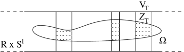
Figure 3. Domains on ${\mathbb{R}}\times S^{1}$.

We further introduce the following space of functions

$$\mathcal{F}_{T}=\Big{\{}\mu\in C^{2}\big{(}\mathrm{cl}(V_{T}),[0,\infty)\big{)}:\Delta\rho+\partial^{2}_{s}\mu|_{\mathcal{Z}_{T}}\geq 0\Big{\}}.$$

We define the following number

$$c_{T}=\inf_{\mu\in\mathcal{F}_{T}}\max_{s\in\mathrm{cl}(V_{T})}\mu(s)\in[0,\infty).$$

Step 1: $\max_{\mathbb{R}\times S^{1}}\rho\leq T+c_{T}$.

For $\epsilon>0$ pick $\mu\in\mathcal{F}_{T}$ such that

$$\max_{\mathrm{cl}(V_{T})}\mu\leq c_{T}+\epsilon.$$

We abbreviate

$$\chi=\rho+\mu|_{\mathcal{Z}_{T}}\in C^{2}\big{(}\mathcal{Z}_{T},\mathbb{R}\big{)}.$$

Note that by definition of $\mu$

$$\Delta\chi\geq 0$$

and hence, since $\mathcal{Z}_{T}$ is compact,

$$\max_{\mathcal{Z}_{T}}\chi=\max_{\partial\mathcal{Z}_{T}}\chi.$$

Using this and the fact that, by definition, $\mu$ is nonnegative, we estimate

$$\max_{\mathcal{Z}_{T}}\rho \leq \max_{\mathcal{Z}_{T}}(\rho+\mu)$$

$$= \max_{\mathcal{Z}_{T}}\chi$$

$$= \max_{\partial\mathcal{Z}_{T}}\chi$$

$$\leq \max_{\partial\mathcal{Z}_{T}}\rho+\max_{\partial\mathcal{Z}_{T}}\mu$$

$$\leq T+c_{T}+\epsilon.$$

Since on the other hand

$$\max_{(\mathbb{R}\times S^{1})\setminus\mathcal{Z}_{T}}\rho\leq T\leq T+c_{T}+\epsilon$$

we conclude that

$$\max_{\mathbb{R}\times S^{1}}\rho\leq T+c_{T}+\epsilon.$$

Because $\epsilon$ was arbitrary Step 1 follows.

Step 2: $c_{T}\leq 4A\delta^{2}$.

We first assume that $\mathrm{cl}(V_{T})$ equals an interval $[0,R]$ for $R>0$. We let $\mu:[0,R]\to[0,\infty)$ be the piecewise $C^{2}$ function which is uniquely determined by the following conditions.

• $\mu(0)=\partial_{s}\mu(0)=0$,

• $\partial^{2}_{s}\mu(s)=\max(\partial_{s}\beta(s),0)$ for every $s\in[0,R]$ at which $\partial_{s}\mu(s)=0$,

• $\partial^{2}_{s}\mu(s)=\partial_{s}\beta(s)$ for every $s\in[0,R]$ at which $\partial_{s}\mu(s)>0$.

Note that the function $\mu$ is monotone and hence, because of its initial condition, nonnegative. Moreover, by construction $\mu$ satisfies

(49) $$\partial^{2}_{s}\mu\geq\partial_{s}\beta$$

and hence, by the inequality in the first line of (47), we conclude that

$$\Delta\rho+\partial^{2}_{s}\mu|_{\mathcal{Z}_{T}}\geq 0.$$

Hence

$$\mu\in\mathcal{F}_{T}.$$

We set $R^{0}=0$ and define recursively for $j\in\mathbb{N}$

$$R_{j} = \inf\big{\{}s\in[R^{j-1},R]:\partial_{s}\beta(s)>0\big{\}},$$

$$R^{j} = \inf\big{\{}s\in(R_{j},R]:\beta(s)=\beta(R_{j})\big{\}},$$

where we understand here that the infimum of the empty set is $R$. We refer to Figure 4 for the construction of the function $\mu$. We denote $I_{j}:=[R_{j},R^{j}]$, $j\geq 1$, and it follows from the definition that

$$\mathrm{supp}({\partial}_{s}\mu)\subset\bigcup_{j=1}^{\infty}I_{j}.$$

We see in particular that $\mu$ is of class $C^{2}$ at all points of $[0,R]$, except for $R^{j}$, $j\geq 1$. However, the map $\mu$ can be smoothened at these points while still preserving condition (49).

Figure 4. The construction of the function $\mu$.

We further put

$$\Delta_{j}=R^{j}-R_{j}\geq 0.$$

We claim the following inequality

(50) $$\sum_{j=1}^{\infty}\Delta_{j}\leq 2\delta.$$

To prove (50) we introduce for $s\in\mathbb{R}$

$$\kappa(s):=\int_{0}^{1}\Big{(}e^{\rho(s,\tau)}-1\Big{)}d\tau.$$

We claim that for every $j\in\mathbb{N}$

(51) $$\int_{R_{j}}^{R^{j}}\kappa(s)ds=0.$$

To see this, first note that if $f(\beta(s_{0}))=0$ for some $s_{0}\in[0,R]$, then the equality in the first line of (47) implies that $\beta$ is constant on $[0,R]$, so $R_{1}=R$ and there is nothing to prove. Hence we may assume $f(\beta(s))>0$ for all $s\in[0,R]$. Pick a function $F:{\mathbb{R}}\to{\mathbb{R}}$ with $F^{\prime}=1/f$. Now $\beta(R_{j})=\beta(R^{j})$ and the equality in the first line of (47) imply the claim:

$$0=F\bigl{(}\beta(R_{j})\bigr{)}-F\bigl{(}\beta(R^{j})\bigr{)}=-\int_{R_{j}}^{R^{j}}\frac{{\partial}_{s}\beta}{f(\beta)}ds=\int_{R_{j}}^{R^{j}}\kappa(s)ds.$$

Next we define the following four subsets of $I_{j}=[R_{j},R^{j}]$:

$$I_{j}^{-}=\{s\in I_{j}:\kappa(s)<0\},\quad I_{j}^{+}=I_{j}\setminus I_{j}^{-},\quad I_{j}^{w}=I_{j}\cap W_{T},\quad I_{j}^{t}=I_{j}\setminus I_{j}^{w}.$$

We observe that, by definition of the wild set and because $I_{j}\subset\mathrm{cl}(V_{T})$, we have

(52) $$\kappa|_{I_{j}^{t}}\geq 1.$$

In particular,

(53) $$I_{j}^{t}\subset I_{j}^{+}.$$

Using (51–53) and the fact that $\kappa\geq-1$ we estimate

(54) $$0=\int_{I_{j}}\kappa=\int_{I_{j}^{-}}\kappa+\int_{I_{j}^{+}}\kappa\geq\int_{I_{j}^{-}}\kappa+\int_{I_{j}^{t}}\kappa\geq-|I_{j}^{-}|+|I_{j}^{t}|.$$

Taking complements in (53) we obtain

(55) $$I_{j}^{-}\subset I_{j}^{w}.$$

Combining (54) and (55) we conclude

(56) $$|I_{j}^{t}|\leq|I_{j}^{w}|.$$

Hence we estimate using (56) and (48)

$$\sum_{j=1}^{\infty}\Delta_{j}=\sum_{j=1}^{\infty}\big{(}|I_{j}^{t}|+|I_{j}^{w}|\big{)}\leq 2\sum_{j=1}^{\infty}|I_{j}^{w}|\leq 2|W_{T}|=2\delta,$$

proving the inequality claimed in (50). By construction of $\mu$ it holds that

(57) $$\{s\,:\,{\partial}^{2}_{s}\mu(s)>0\}\subset\mathrm{supp}\big{(}\partial_{s}\mu\big{)}\subset\bigcup_{j=1}^{\infty}I_{j}.$$

Moreover, we observe using the equation in the first line of (47) and the assumption that the function $f$ is bounded from above by $A$ that

(58) $$\max\big{(}\partial^{2}_{s}\mu\big{)}\leq\max\big{(}\max\,\partial_{s}\beta,0\big{)}\leq A.$$

From (50),(57), and (58) we deduce

(59) $$\max\big{(}\partial_{s}\mu\big{)}\leq 2\delta A.$$

Combining (59) again with (50) and (57) we conclude that

$$\max\mu\leq 4A\delta^{2},$$

and hence

$$c_{T}\leq 4A\delta^{2}.$$

This finishes the proof of Step 2 in the case that $\mathrm{cl}(V_{T})$ is an interval. In the general case $\mathrm{cl}(V_{T})$ is a countable union of intervals and, possibly, accumulation points. Ignoring the latter, we can apply the previous construction to each component, always setting $\mu={\partial}_{s}\mu=0$ at the left end point of each interval. This concludes the proof of Proposition 5.3 and hence of Proposition 5.2. ∎

5.3. A useful dichotomy

In this subsection we prove a general result which says that, under certain hypotheses, the Morse complex of a functional $f:X\times{\mathbb{R}}\to{\mathbb{R}}$ splits into two subcomplexes for small/large $\eta$ which are not connected by gradient flow lines. In the next subsection we will apply this result to the Rabinowitz functional $A_{H,b,c}:{\mathcal{L}}\times{\mathbb{R}}\to{\mathbb{R}}$.

Let $(X,g_{X})$ be a (maybe infinite dimensional) Riemannian manifold and $f\colon X\times\mathbb{R}\to\mathbb{R}$ a smooth function. We consider on the manifold $X\times\mathbb{R}$ the Riemannian metric $g=g_{X}\oplus g_{\mathbb{R}}$ where $g_{\mathbb{R}}$ is the standard metric on $\mathbb{R}$. We denote by $\nabla f$ the gradient of $f$ with respect to the metric $g$ and by $||\cdot||$ the norm with respect to the metric $g$.

Definition 5.4.

We say that $f$ is of Rabinowitz type if there exists a quadruple of positive constants $(\epsilon,D,c_{1},c_{2})$ such that for all $(x,\eta)\in X\times\mathbb{R}$ the following two conditions hold

(i):

$||\nabla f(x,\eta)||\leq\epsilon,\,\,|\eta|\leq D\,\,\Longrightarrow|\eta|\leq c_{1}\big{(}|f(x,\eta)|+||\nabla f(x,\eta)||\big{)}$;

(ii):

$|\partial_{\eta}f(x,\eta)|\leq c_{2}$ along gradient flow lines connecting critical points.

We refer to the quadruple $(\epsilon,D,c_{1},c_{2})$ as a Rabinowitz quadruple for $f$.

In the following we assume that $f$ is of Rabinowitz type and $(\epsilon,D,c_{1},c_{2})$ is a fixed Rabinowitz quadruple for $f$. Moreover, we assume without loss of generality that

$$D>c_{1}\epsilon.$$

We define the functions $b_{\pm}:{\mathbb{R}}_{+}\to{\mathbb{R}}$,

$$b_{-}(a):=c_{1}(a+\epsilon)+\frac{2ac_{2}}{\epsilon^{2}},\qquad b_{+}(a):=D-\frac{2ac_{2}}{\epsilon^{2}}.$$

We further introduce the quantity

$$\kappa:=\frac{\epsilon^{2}(D-c_{1}\epsilon)}{c_{1}\epsilon^{2}+4c_{2}}$$

and note that

$$b_{-}(a)<b_{+}(a)\qquad\text{for }a<\kappa.$$

Now assume that $w=(x,\eta)\in C^{\infty}(\mathbb{R},X\times\mathbb{R})$ is a gradient flow line of $f$, i.e. a solution of the ODE

$$\partial_{s}w(s)=\nabla f(w(s)),\quad s\in\mathbb{R}.$$

For a gradient flow line we abbreviate

$$A_{w}=\sup_{s\in\mathbb{R}}\big{|}f(w(s))\big{|}.$$

We refer to $A_{w}$ as the absolute action of $w$. The following proposition shows that there is a dichotomy of gradient flow lines of Rabinowitz type functions of small absolute action into gradient flow lines with large $|\eta|$ and small $|\eta|$.

Proposition 5.5.

Suppose that $f$ is of Rabinowitz type with Rabinowitz quadruple $(\epsilon,D,c_{1},c_{2})$ and define $b_{\pm}(a),\kappa$ as above. Let $w=(x,\eta)\in C^{\infty}(\mathbb{R},X\times\mathbb{R})$ be a gradient flow line of $f$ with absolute action $A_{w}=a<\kappa$. Then exactly one of the following two cases holds:

(i):

$|\eta(s)|\leq b_{-}(a)$ for all $s\in\mathbb{R}$;

(ii):

$|\eta(s)|>b_{+}(a)$ for all $s\in\mathbb{R}$.

Proof.

For $\sigma\in\mathbb{R}$ we abbreviate

$$\tau(\sigma)=\inf\big{\{}\tau\geq 0:||\nabla f(w(\sigma+\tau))||\leq\epsilon\big{\}}.$$

Using the gradient flow equation we estimate

$$\epsilon^{2}\tau(\sigma) \leq \int_{\sigma}^{\sigma+\tau(\sigma)}||\nabla f(w(s))||^{2}ds$$

$$= \int_{\sigma}^{\sigma+\tau(\sigma)}\frac{d}{ds}f(w(s))ds$$

$$= f\big{(}w(\sigma+\tau(\sigma))\big{)}-f\big{(}w(\sigma)\big{)}$$

$$\leq 2A_{w},$$

implying that

(60) $$\tau(\sigma)\leq\frac{2A_{w}}{\epsilon^{2}}.$$

Since the metric $g$ on $X\times\mathbb{R}$ is of product form, the gradient flow equation for $\eta$ reads

$$\partial_{s}\eta=\partial_{\eta}f(w).$$

Hence using assertion (ii) in Definition 5.4 we obtain that

(61) $$|\partial_{s}\eta|\leq c_{2}.$$

Using (60) and (61) we get

(62) $$\big{|}\eta(\sigma)-\eta(\sigma+\tau(\sigma))\big{|}\leq\int_{\sigma}^{\sigma+\tau(\sigma)}|\partial_{s}\eta|ds\leq c_{2}\tau(\sigma)\leq\frac{2c_{2}A_{w}}{\epsilon^{2}}.$$

We distinguish the following two cases.

Case 1: $\big{|}\eta(\sigma+\tau(\sigma))\big{|}>D$.

In this case we obtain using (62) that

$$\big{|}\eta(\sigma)\big{|}\geq\big{|}\eta(\sigma+\tau(\sigma))\big{|}-\frac{2c_{1}A_{w}}{\epsilon^{2}}>D-\frac{2c_{2}A_{w}}{\epsilon^{2}}=b_{+}(A_{w}).$$

Case 2: $\big{|}\eta(\sigma+\tau(\sigma))\big{|}\leq D$.

In this case we estimate using the assertion (i) in Definition 5.4 and again inequality (62)

$$\big{|}\eta(\sigma)\big{|}\leq\big{|}\eta(\sigma+\tau(\sigma))\big{|}+\frac{2c_{2}A_{w}}{\epsilon^{2}}\leq c_{1}(A_{w}+\epsilon)+\frac{2c_{2}A_{w}}{\epsilon^{2}}=b_{-}(A_{w}).$$

Since $b_{+}(A_{w})>b_{-}(A_{w})$, continuity of $\eta$ implies that either $|\eta(s)|\leq b_{-}(A_{w})$ for all $s\in\mathbb{R}$ or $|\eta(s)|>b_{+}(A_{w})$ for all $s\in\mathbb{R}$. This proves Proposition 5.5. ∎

5.4. Proof of Theorem 5.1

Let us fix $-\infty<\alpha<\beta<\infty$ such that $\alpha,\beta\notin{\rm Spec}(M,\lambda)$, and a function $h$ satisfying $h^{\prime}(r)\geq 0$ for $r>0$ and $h(r)=r-1$ for $r\geq 1/2$. We consider Rabinowitz functionals $A_{H,b,c}$ for $H=h(r)$, $c\equiv 0$, and $b$ satisfying

(63) $$0\leq b^{\prime}(\eta)\leq 1,\qquad b(\eta)=\eta\text{ for }|\eta|\leq D,$$

with a constant

$$D>2\max(|\alpha|,|\beta|)$$

to be determined later.

Recall that critical points $(x,\eta)$ of $A_{H,b,0}$ with $x=(y,r)$ satisfy

$$\left\{\begin{array}[]{l}\dot{y}=b(\eta)h^{\prime}(r)R,\\ b^{\prime}(\eta)h(r)=0.\end{array}\right.$$

The action of such a critical point is

$$A_{H,b,0}(x,\eta)=b(\eta)(rh^{\prime}(r)-h(r)).$$

(in the region $\widehat{V}\setminus M\times{\mathbb{R}}_{+}$, the formula is to be read via the convention $h^{\prime}(0)=0$ and $h(0)=\mathrm{ct.}$). There are two types of critical points as above:

Type 1: $b^{\prime}(\eta)\neq 0$. In this case $h(r)=0$ and hence $r=1$ and $A_{H,b,0}(x,\eta)=b(\eta)$.

Type 2: $b^{\prime}(\eta)=0$. In this case suppose first $r\geq 1/2$. Then the action $A_{H,b,0}(x,\eta)=b(\eta)$ cannot lie in the interval $(\alpha,\beta)$ because $b(\eta)=\eta$ on this interval. Hence we must have $r\leq 1/2$, so that $h(r)\leq-1/2$ and therefore $rh^{\prime}(r)-h(r)\geq-h(r)\geq 1/2$. This implies $|A_{H,b,0}|\geq|b(\eta)|/2\geq D/2$, and the action does not lie in $(\alpha,\beta)$.

We thus proved that all critical points with action in $(\alpha,\beta)$ satisfy $r=1$. Hence by Proposition 5.2 there exists a constant $c_{2}$ depending only on $\beta-\alpha$ such that $r(s,t)\leq c_{2}$ along all gradient flow lines of $A_{H,b,0}$ connecting critical points with action in $(\alpha,\beta)$.

By the proof of Proposition 3.2 in [9] there exist constants ${\varepsilon},c_{1}>0$ such that for the unperturbed Rabinowitz functional the following holds:

$$||\nabla A_{H,\eta,0}(x,\eta)||\leq\epsilon\Longrightarrow|\eta|\leq c_{1}\big{(}|A_{H,\eta,0}(x,\eta)|+||\nabla A_{H,\eta,0}(x,\eta)||\big{)}.$$

Since $b(\eta)=\eta$ for $|\eta|\leq D$, for the perturbed Rabinowitz functional this implies

$$||\nabla A_{H,b,0}(x,\eta)||\leq\epsilon,\ |\eta|\leq D\Longrightarrow|\eta|\leq c_{1}\big{(}|A_{H,b,0}(x,\eta)|+||\nabla A_{H,b,0}(x,\eta)||\big{)}.$$

This shows that $A_{H,b,0}$ is of Rabinowitz type in the sense of the previous subsection with Rabinowitz quadruple $({\varepsilon},D,c_{1},c_{2})$. Moreover, note the crucial fact that the constants ${\varepsilon},c_{1},c_{2}$ work for all functions $b$ satisfying (63), independently of $D$! Thus we can choose $D=D(\alpha,\beta)$ so large that the quantities $\kappa$ and $b_{\pm}(a)$ defined as in the previous section satisfy

$$\kappa>\max(|\alpha|,|\beta|),\qquad b_{-}(\kappa)>\max(|\alpha|,|\beta|).$$

This implies that for $a<\kappa$ we have $b_{-}(a)<b_{+}(a)$ and

$$b_{+}(a)>b_{+}(\kappa)\geq b_{-}(\kappa)>\max(|\alpha|,|\beta|).$$

On the other hand, the discussion above shows that all critical points $(x,\eta)$ with action in $(\alpha,\beta)$ satisfy

$$A_{H,b,0}(x,\eta)=b(\eta)=\eta\in(\alpha,\beta).$$

Now we apply Proposition 5.5 to the functional $A_{H,b,0}:U\to{\mathbb{R}}$ with

$$U:=\{(x,\eta)\in{\mathcal{L}}\times{\mathbb{R}}\mid A_{H,b,0}(x,\eta)\in(\alpha,\beta)\}.$$

The preceding discussion shows that case (ii) in Proposition 5.5 does not occur, so along every gradient flow line connecting critical points in $(\alpha,\beta)$ we have

$$|\eta(s)|\leq b_{-}(\kappa).$$

Now a short computation shows

$$b_{-}(\kappa)=D\left(\frac{1}{2}+O({\varepsilon})\right)+O({\varepsilon}),$$

where the implicit constants in $O({\varepsilon})$ depend only on $c_{1}$ and $c_{2}$. Assuming without loss of generality that ${\varepsilon}$ is sufficiently small, we may therefore assume $b_{-}(\kappa)<D$. The resulting estimate

$$|\eta(s)|<D$$

shows that gradient flow lines of $A_{H,b,0}$ connecting critical points with action in $(\alpha,\beta)$ stay in the region where $b(\eta)=\eta$ and therefore agree with gradient flow lines of the unperturbed Rabinowitz functional $A_{H,\eta,0}$. Hence the chain complexes of $A_{H,b,0}$ and $A_{H,\eta,0}$ in the action interval $(\alpha,\beta)$ coincide and we conclude

$$FH^{(\alpha,\beta)}(A_{H,\eta,0})\cong FH^{(\alpha,\beta)}(A_{H,b,0}).$$

This conclusion holds for all functions $b$ satisfying (63), in particular for functions $b=b_{A}$ as in Lemma 4.7 with $A\geq D(\alpha,\beta)+1$. This concludes the proof of Theorem 5.1. $\square$

6. Proof of the main result

In this section we prove Theorem 1.5 in the Introduction, i.e. the isomorphism

$$RFH_{*}(V)\simeq\check{SH}_{*}(V).$$

For this we consider deformed Rabinowitz action functionals of the form

$$A_{H,b,c}(x,\eta)=\int_{0}^{1}x^{*}\lambda-b(\eta)\int_{0}^{1}H(x(t))dt+c(\eta),$$

with $H:\widehat{V}\to{\mathbb{R}}$ and $b,c:{\mathbb{R}}\to{\mathbb{R}}$ smooth functions.

We start with a summary of what we achieved in Sections 4 and 5. Let $(\alpha,\beta)$ be a fixed action interval, such that $|\alpha|,|\beta|\notin\mathrm{Spec}(M,\lambda)$. By definition, we have $RFH_{*}^{(\alpha,\beta)}(V)=FH_{*}^{(\alpha,\beta)}(A_{H,\eta,0})$ for a defining Hamiltonian $H:\widehat{V}\to{\mathbb{R}}$ which is constant at infinity. In the sequel, we only consider Hamiltonians of the form $H=h(r)$, where $r\in{\mathbb{R}}_{+}$ is the second coordinate in the symplectization $M\times{\mathbb{R}}_{+}$. By Proposition 4.13, we also have

$$RFH_{*}^{(\alpha,\beta)}(V)=FH_{*}^{(\alpha,\beta)}(A_{H,\eta,0}),$$

for a Hamiltonian $H=h(r)$ with $h(r)=r-1$ for $r\geq 1/2$. By Theorem 5.1 we have

(64) $$FH_{*}^{(\alpha,\beta)}(A_{H,\eta,0})=FH_{*}^{(\alpha,\beta)}(A_{H,b,0}),$$

with $b=b_{A}$ as in (38) and $A\notin\mathrm{Spec}(M,\lambda)$ sufficiently large. Finally, by Proposition 4.15 the right hand side of (64) is isomorphic to

$$FH_{*}^{(\alpha,\beta)}(A_{\widetilde{H},\widetilde{b},c})$$

for every triple $(\widetilde{H},\widetilde{b},c)$ satisfying (42) that can be connected to $(H,b,0)$ by a homotopy of such triples during which the critical points do not cross the boundary of the action interval $(\alpha,\beta)$, and form a compact set.

In this section we construct a homotopy to a triple $(\widetilde{H},1,c)$ for which $FH_{*}^{(\alpha,\beta)}(A_{\widetilde{H},1,c})=\check{SH}_{*}^{(\alpha,\beta)}(V)$. We achieve this in five steps, as follows.

Step 1. We rescale $(H,b,0)$ to $(\mu H,b/\mu,0)$ for a suitable $\mu>0$.

Step 2. We replace $(\mu H,b/\mu,0)$ by $(\mu H,b/\mu,c)$ for a suitable $c$ (Figure 6).

Step 3. We replace $(\mu H,b/\mu,c)$ by $(K,b/\mu,c)$, where $K$ is a flattening of $H$ near $r=1$ (Figure 5).

Step 4. We homotope the action functional $A_{K,b/\mu,c}$ to $A_{|K|,1,c}$.

Step 5. By our special choice of $c$ and $K$, we have

$$FH_{*}^{(\alpha,\beta)}(A_{|K|,1,c})=FH_{*}^{(\alpha,\beta)}(|K|)=\check{SH}_{*}^{(\alpha,\beta)}(V).$$

Proof of Theorem 1.5.

Let $-\infty<\alpha<\beta<+\infty$ be fixed, such that $|\alpha|,|\beta|\notin\mathrm{Spec}(M,\lambda)$. Given $0<\delta<1$ and $\mu>0$ we define the following Hamiltonians. Let $H=H_{\delta}:\widehat{V}\to{\mathbb{R}}$ be such that, up to smooth approximation in the neighbourhood of $\{\delta\}\times M$, it satisfies (Figure 5)

$$\left\{\begin{array}[]{ll}H\equiv\delta-1&\mbox{on }V\setminus[\delta,1]\times M,\\ H(r,x)=h(r)&\mbox{on }[\delta,\infty)\times M,\qquad\qquad\mbox{with }h(r)=r-1.\end{array}\right.$$

Let $K=K_{\delta,\mu}:\widehat{V}\to{\mathbb{R}}$ be such that, up to smooth approximation in the neighbourhood of $\{\delta\}\times M$ and $\{1\}\times M$, it satisfies (Figure 5)

$$\left\{\begin{array}[]{ll}K\equiv\mu(\delta-1)&\mbox{on }V\setminus\,[\delta,1]\times M,\\ K(r,x)=k(r)&\mbox{on }[\delta,\infty)\times M,\end{array}\right.$$

with $k(1)=k^{\prime}(1)=0$ and

$$\left\{\begin{array}[]{cl}k^{\prime}>0&\mbox{for }r\in]\delta,\infty)\setminus\{1\},\\ k(r)=\mu(r-1)&\mbox{outside small neighbourhoods of }\delta\mbox{ and }1.\end{array}\right.$$

Figure 5. The Hamiltonians $H$, $K$, and $|K|$.

We define now $c:{\mathbb{R}}\to[0,\infty)$ to be an even function such that (Figure 6)

(65) $$\left\{\begin{array}[]{l}c(0)=0,\\ 0<\sup c=c_{0}<\infty,\\ c^{\prime}(\eta)=0\mbox{ iff }\eta=0.\end{array}\right.$$

Figure 6. A suitable function $c$.

We recall that, given $A>0$, we defined in Section 4.3 the function $b=b_{A}:{\mathbb{R}}\to{\mathbb{R}}$ such that, up to smooth approximation in the neighbourhood of $\eta=\pm A$, it satisfies the conditions (Figure 7)

$$\left\{\begin{array}[]{ll}b\equiv-A,&\eta\leq-A,\\ b(\eta)=\eta,&-A\leq\eta\leq A,\\ b\equiv A,&A\leq\eta.\end{array}\right.$$

Figure 7. The function $b$.

For any $p\notin\mathrm{Spec}(M,\lambda)$, we recall that $\eta_{p}>0$ is the distance from $p$ to the closed set $\mathrm{Spec}(M,\lambda)$. Let $A(\alpha,\beta)>0$ be the constant from Theorem 5.1, and let us denote $T_{0}=\min\mathrm{Spec}(M,\lambda)>0$.

Assumptions.

• (assumption on $\mu$ and $A$) We require that $\mu=A\notin\mathrm{Spec}(M,\lambda)$ and

  $$\mu=A\geq 10\max\{|\alpha|,|\beta|,1,T_{0},A(\alpha,\beta)\}.$$

  (we distinguish in notation between $\mu$ and $A$ since they play different roles).

• (assumption on $\delta$) We require $\delta\leq\frac{1}{2}$.

• (assumption on $b$) The smoothing of $b$ takes place in small enough intervals near $\pm A$, so that

  $$0<b^{\prime}(\eta)<1\ \Longrightarrow\ b(\eta)\in[-A,-A+\eta_{A})\,\cup\,(A-\eta_{A},A].$$

• Let

  $$d_{A,\alpha,\beta}:=\min\{|p-q|\ :\ p\neq q\in\mathrm{Spec}(M,\lambda)\cup\{0,\alpha,\beta\},\ p,q\leq A\}>0.$$

  Let ${\varepsilon}_{0}>0$ be such that

  $$\mu-\eta_{\mu}\leq(1-{\varepsilon}_{0})\mu<\mu.$$

  Let

  (66) $${\varepsilon}_{A,\alpha,\beta}:=d_{A,\alpha,\beta}/10A.$$

  It follows from the definition of $d_{A,\alpha,\beta}$ that ${\varepsilon}_{A,\alpha,\beta}$ satisfies the condition

  (67) $$|r-1|<{\varepsilon}_{A,\alpha,\beta}\ \Rightarrow\ |rp-p|<d_{A,\alpha,\beta},\ \forall\ p\in\mathrm{Spec}(M,\lambda)\,\cap\,(0,A).$$

• (assumption on $c$) We require that

  $$\sup|c|\leq\min\{\frac{1}{2},\ d_{A,\alpha,\beta}/10\}$$

  and

  $$\sup|c^{\prime}|\leq\min\{\frac{1}{2},\ {\varepsilon}_{0}{\varepsilon}_{A,\alpha,\beta}d_{A,\alpha,\beta}/10A^{2}\}.$$

• (assumption on $k$) Let $c_{1}:=\frac{1}{2}\min\{|c^{\prime}(\eta)|\ :\ |\eta-A|\leq\eta_{A}\mbox{ or }|\eta+A|\leq\eta_{A}\}$. Let $\bar{b}(\eta):=b(\eta)/\mu$, and let $c_{2}>0$ be such that

  $$|c^{\prime}(\eta)/\bar{b}^{\prime}(\eta)|\leq c_{2}\ \Rightarrow\ |\bar{b}(\eta)|<T_{0}/\mu.$$

  Let $c_{3}:=\min(c_{1},c_{2})$. We require that, in the neighbourhood of $r=1$, we have

  $$|k(r)|\geq c_{3}\ \Rightarrow\ k^{\prime}(r)=\mu.$$

  (This means that $k$ differs from a linear function only in a small neighbourhood of $r=1$).

Before proving Steps 1 to 5, we recall that critical points of $A_{H,b,c}$ are pairs $(x,\eta)$ such that

$$\left\{\begin{array}[]{l}\dot{x}=b(\eta)X_{H},\\ b^{\prime}(\eta)\int H(x(t))dt=c^{\prime}(\eta).\end{array}\right.$$

This is equivalent to the following:

1. Either $b^{\prime}(\eta)=0$, in which case $c^{\prime}(\eta)=0$ and $\dot{x}=b(\eta)X_{H}$,

2. or $b^{\prime}(\eta)\neq 0$, in which case $\dot{x}=b(\eta)X_{H}$ and

   $$x(t)\in H^{-1}(c^{\prime}(\eta)/b^{\prime}(\eta)),\quad t\in S^{1}.$$

We refer to $(x,\eta)$ as a critical point of Type (1), respectively Type (2). In case $H=h(r)$, critical points $(x,\eta)$ appear on levels $r=\mathrm{ct.}$ and have action

$$A_{H,b,c}(x,\eta)=b(\eta)\big{(}rh^{\prime}(r)-h(r)\big{)}+c(\eta).$$

As above, we use the convention $h^{\prime}(0)=0$ and $h(0)=H(x)$.

Step 1. We have a canonical identification of complexes

$$CF_{*}^{(\alpha,\beta)}(A_{H,b,0})=CF_{*}^{(\alpha,\beta)}(A_{\mu H,b/\mu,0})$$

This follows directly from the equality $A_{H,b,0}=A_{\mu H,b/\mu,0}$. $\square$

Remark. From now on the functions $\mu H$ and $b/\mu$ remain unchanged outside a compact set, so that moduli spaces of gradient trajectories are compact modulo breaking (Proposition 4.15) and the Rabinowitz-Floer homology groups are well-defined.

Step 2. There is a chain map inducing an isomorphism in homology

$$CF_{*}^{(\alpha,\beta)}(A_{\mu H,b/\mu,0})\to CF_{*}^{(\alpha,\beta)}(A_{\mu H,b/\mu,c}).$$

We denote $\bar{H}:=\mu H$, $\bar{h}:=\mu h$, $\bar{b}:=b/\mu$, and consider the homotopy $A_{s}=A_{\bar{H},\bar{b},\rho(s)c}$, with $s\in{\mathbb{R}}$ and $\rho:{\mathbb{R}}\to[0,1]$ a smooth increasing function, equal to $0$ near $-\infty$ and equal to $1$ near $+\infty$. To prove that the induced chain map is a quasi-isomorphism it is enough to examine the action of the critical points of each $A_{s}$, and show that none of these actions crosses the boundary of the interval $(\alpha,\beta)$. We prove that the actions of critical points of $A_{\bar{H},\bar{b},c}$ stay away from $\alpha$ and $\beta$ (the same computation shows that this holds true for any $A_{s}$ since $0\leq\rho\leq 1$).

A critical point $(x,\eta)$ of $A_{\bar{H},\bar{b},c}$ with $x$ on level $r$ satisfies

$$\left\{\begin{array}[]{l}\dot{x}=\bar{b}(\eta)X_{\bar{H}},\\ \bar{b}^{\prime}(\eta)\bar{h}(r)=c^{\prime}(\eta),\end{array}\right.$$

so that $|\eta|<A$ and $\bar{b}^{\prime}(\eta)\neq 0$. We distinguish several cases according to the value of the strictly increasing function $f(\eta)=c^{\prime}(\eta)/\bar{b}^{\prime}(\eta)$ on the interval $(-A,A)$ (see Figure 8). We have $\bar{h}(r)=f(\eta)$ and the cases that we distinguish correspond to the various types of orbits of $\bar{H}$.

Case 1. $f(\eta)=\mu(\delta-1)\leq-\frac{\mu}{2}$. Then we must have $\eta\in[-A,-A+\eta_{A}]$, because $f(\eta)=\mu c^{\prime}(\eta)>-\frac{\mu}{2}$ for $\eta\in[-A+\eta_{A},0]$. As a consequence $\bar{b}(\eta)$ is close to $-1$ (here we use for the first time that $\mu=A$). Moreover $X_{\bar{H}}=0$, $x$ is constant and the action is $A_{\bar{H},\bar{b},c}(x,\eta)=-\bar{b}(\eta)\bar{h}(r)+c(\eta)\leq-\frac{\mu}{2}+\frac{1}{2}<\alpha-1$.

Case 2. $f(\eta)$ is close to $\mu(\delta-1)$ and the slope of $\bar{h}$ varies between $0$ and $\mu$, so that $x$ lives on a level $r$ close to $\delta$. As in Case 1 we get that $\eta\in[-A,-A+\eta_{A}]$, $\bar{b}(\eta)$ is close to $-1$ and the action satisfies $A_{\bar{H},\bar{b},c}(x,\eta)=\bar{b}(\eta)(\bar{h}^{\prime}(r)r-h(r))+c(\eta)<-\bar{b}(\eta)\bar{h}(r)+c(\eta)<\alpha-1$.

Case 3. $f(\eta)$ is bigger than $\mu(\delta-1)$, and $\bar{h}^{\prime}=\mu$. Then $\eta\in[-A+\eta_{A},A-\eta_{A}]$, $\bar{b}(\eta)=\eta/\mu$ and $\bar{b}^{\prime}(\eta)=1/\mu$ (otherwise $\bar{b}(\eta)\simeq\pm 1$ and, since $\mu\notin\mathrm{Spec}(M,\lambda)$, there are no solutions of $\dot{x}=\bar{b}(\eta)\bar{h}^{\prime}(x)R_{\lambda}=\bar{b}(\eta)\mu R_{\lambda}$). Such a critical point $(x,\eta)$ satisfies

$$\left\{\begin{array}[]{l}\dot{x}=\eta R_{\lambda},\\ \bar{H}(x)=\mu c^{\prime}(\eta),\end{array}\right.$$

and the set of critical points in Case 5 is in bijective correspondence with the set of critical points of $A_{H,b,0}=A_{\bar{H},\bar{b},0}$ with action in $[-A+\eta_{A},A-\eta_{A}]$ (the correspondence assigns to $(x,\eta)$ the pair $(\widetilde{x},\eta)$, where $\widetilde{x}$ represents the same characteristic as $x$, but located on the level $r=1$ instead of $r=\bar{h}^{-1}(\mu c^{\prime}(\eta))=1+c^{\prime}(\eta)$). The action is $A_{\bar{H},\bar{b},c}(x,\eta)=\eta r-\eta c^{\prime}(\eta)+c(\eta)=\eta+c(\eta)$. By assumption we have $\sup|c|\leq d_{A,\alpha,\beta}/2$, and this ensures that

$$|A_{\bar{H},\bar{b},c}(x,\eta)-A_{\bar{H},\bar{b},0}(\widetilde{x},0)|\leq d_{A,\alpha,\beta}.$$

The action of the critical points therefore varies by at most $d_{A,\alpha,\beta}$ during the deformation, and cannot cross the bounds of the interval $(\alpha,\beta)$. $\square$

Figure 8. The function $c^{\prime}/\bar{b}^{\prime}$.

Step 3. There is a chain map inducing an isomorphism in homology

$$CF_{*}^{(\alpha,\beta)}(A_{\mu H,b/\mu,c})\to CF_{*}^{(\alpha,\beta)}(A_{K,b/\mu,c}).$$

We use the notation $\bar{H}=\mu H$, $\bar{h}=\mu h$, $\bar{b}=b/\mu$ from Step 2, and recall that $K=k(r)$ on $[\delta,\infty)$. Let $\rho:{\mathbb{R}}\to[0,1]$ be a smooth increasing function equal to $0$ near $-\infty$ and equal to $1$ near $+\infty$. We consider the homotopy $A_{s}=A_{H_{s},\bar{b},c}$, $s\in{\mathbb{R}}$ with $H_{s}=(1-\rho(s))\bar{H}+\rho(s)K$. To prove that the induced chain map is a quasi-isomorphism we show that, under our assumptions on the perturbation $k$ of $\bar{h}$, the critical points of $A_{s}$ stay fixed during the homotopy together with their action. We prove this for $A_{\infty}=A_{K,\bar{b},c}$, and the same computations work for any $s\in{\mathbb{R}}$ since we do not use the fact that $k^{\prime}(1)=0$.

A critical point $(x,\eta)$ of $A_{K,\bar{b},c}$ with $x$ on level $r$ satisfies

$$\left\{\begin{array}[]{l}\dot{x}=\bar{b}(\eta)X_{K},\\ \bar{b}^{\prime}(\eta)k(r)=c^{\prime}(\eta),\end{array}\right.$$

so that $|\eta|<A$ and $\bar{b}^{\prime}(\eta)\neq 0$. As in Step 2 we distinguish several cases according to the value of $f(\eta)=c^{\prime}(\eta)/\bar{b}^{\prime}(\eta)$, and it is clear that critical points falling in Cases 1 and 2 of Step 2 are the same, with the same action throughout the homotopy.

We now examine critical points $(x,\eta)$ such that $f(\eta)$ is bigger than $\mu(\delta-1)$. The critical points such that $k^{\prime}(r)=\mu$ are the same as those of $A_{\bar{H},\bar{b},c}$, and have the same action. Thus, the relevant new situation is when the value of $k^{\prime}(r)$ is strictly smaller than $\mu$.

We first claim that $\eta\in[-A+\eta_{A},A-\eta_{A}]$. Otherwise $\bar{b}(\eta)\simeq\pm 1$ and $|k(r)|=|c^{\prime}(\eta)/\bar{b}^{\prime}(\eta)|\geq c_{1}$. Then, by assumption, we have $k^{\prime}(r)=\mu\notin\mathrm{Spec}(M,\lambda)$, so that there are no solutions of $\dot{x}=\bar{b}(\eta)X_{K}=\bar{b}(\eta)\mu R_{\lambda}$.

We now claim that the only critical points $(x,\eta)$ such that $x$ lies on a level $r>\delta$ with $k^{\prime}(r)<\mu$ are of the form $(x,0)$ and satisfy $r=1$ (moreover, they have the same action along the homotopy). Indeed, by our assumption on $k$ we must have $|k(r)|\leq c_{2}$, so that $|\bar{b}(\eta)|\mu$ is smaller than $T_{0}$ and any solution of the equation $\dot{x}=\bar{b}(\eta)k^{\prime}(r)R_{\lambda}$ must be constant. Thus, we either have $k^{\prime}(r)=0$ and $r=1$, or $\bar{b}(\eta)=0$ and $\eta=0$. These conditions are equivalent because $\bar{b}^{\prime}(\eta)k(r)=c^{\prime}(\eta)$, and this completes the proof. $\square$

Step 4. There is a chain map inducing an isomorphism in homology

$$CF_{*}^{(\alpha,\beta)}(A_{K,b/\mu,c})\to CF_{*}^{(\alpha,\beta)}(A_{|K|,1,c}).$$

For $0\leq{\varepsilon}\leq 1$ we denote

$$A_{\varepsilon}(x,\eta) := (1-{\varepsilon})A_{K,\bar{b},c}(x,\eta)+{\varepsilon}A_{|K|,1,c}(x,\eta)$$

$$= \int x^{*}(r\lambda)-(1-{\varepsilon})\bar{b}(\eta)\int k(r)-{\varepsilon}\int|k(r)|+c(\eta).$$

Let $\rho:{\mathbb{R}}\to[0,1]$ be a smooth increasing function, equal to $0$ near $-\infty$ and equal to $1$ near $+\infty$. We prove the following claim, which implies that the chain map induced by the homotopy $A_{\rho(s)}$, $s\in{\mathbb{R}}$ is a quasi-isomorphism.

For each critical point $(x^{\varepsilon},\eta^{\varepsilon})$ of $A_{\varepsilon}$ there is a critical point $(x^{1},0)$ of $A_{1}$ such that $|A_{\varepsilon}(x^{\varepsilon},\eta^{\varepsilon})-A_{1}(x^{1},0)|\leq d_{A,\alpha,\beta}$.

The claim is obvious for ${\varepsilon}=1$, so that we can assume without loss of generality that $0\leq{\varepsilon}<1$. The equations for a critical point $(x^{\varepsilon},\eta^{\varepsilon})$ of $A_{\varepsilon}$ on level $r^{\varepsilon}$ are

$$\left\{\begin{array}[]{l}\dot{x}^{\varepsilon}=\big{(}(1-{\varepsilon})\bar{b}(\eta^{\varepsilon})k^{\prime}(r^{\varepsilon})+{\varepsilon}|k|^{\prime}(r^{\varepsilon})\big{)}R_{\lambda},\\ (1-{\varepsilon})\bar{b}^{\prime}(\eta^{\varepsilon})k(r^{\varepsilon})=c^{\prime}(\eta^{\varepsilon}).\end{array}\right.$$

We denote $\bar{b}_{\varepsilon}:=(1-{\varepsilon})\bar{b}+{\varepsilon}$ and distinguish three cases.

Case I. $\eta^{\varepsilon}=0$. Then $r^{\varepsilon}=1$, $k^{\prime}(r^{\varepsilon})=|k|^{\prime}(r^{\varepsilon})=0$, $x^{\varepsilon}=\mathrm{ct.}$ and $A_{\varepsilon}(x^{\varepsilon},0)=0$. The claim holds with $x^{1}:=x^{\varepsilon}$.

Case II. $\eta^{\varepsilon}>0$. Then $r^{\varepsilon}>1$, $|k|(r^{\varepsilon})=k(r^{\varepsilon})$, we have

$$\left\{\begin{array}[]{l}\dot{x}^{\varepsilon}=\bar{b}_{\varepsilon}(\eta^{\varepsilon})k^{\prime}(r^{\varepsilon})R_{\lambda},\\ (1-{\varepsilon})\bar{b}^{\prime}(\eta^{\varepsilon})k(r^{\varepsilon})=c^{\prime}(\eta^{\varepsilon}),\end{array}\right.$$

and the action is $A_{\varepsilon}(x^{\varepsilon},\eta^{\varepsilon})=\bar{b}_{\varepsilon}(\eta^{\varepsilon})(r^{\varepsilon}k^{\prime}(r^{\varepsilon})-k(r^{\varepsilon}))+c(\eta^{\varepsilon})$.

Case II.i. If $0\leq{\varepsilon}<1-{\varepsilon}_{0}$ we distinguish the following cases.

Case II.i.1. $\eta^{\varepsilon}\in(0,A-\eta_{A}]$. Then $c^{\prime}/(1-{\varepsilon})\bar{b}^{\prime}\leq\mu\sup|c^{\prime}|/{\varepsilon}_{0}$ is so small that $\bar{b}_{\varepsilon}(\eta^{\varepsilon})k(r^{\varepsilon})\leq\mu k(r^{\varepsilon})\leq d_{A,\alpha,\beta}/10$. Moreover, we have $\mu(r^{\varepsilon}-1)\simeq k(r^{\varepsilon})=c(\eta^{\varepsilon})/(1-{\varepsilon})\bar{b}^{\prime}(\eta^{\varepsilon})\leq\mu\sup|c^{\prime}|/{\varepsilon}_{0}\leq d_{A,\alpha,\beta}/10\mu$, which implies $1<r^{\varepsilon}\leq 1+d_{A,\alpha,\beta}/10\mu^{2}\leq 1+{\varepsilon}_{A,\alpha,\beta}$, where ${\varepsilon}_{A,\alpha,\beta}=d_{A,\alpha,\beta}/10\mu$ was introduced in (66). Since $1\leq r^{\varepsilon}\leq 1+{\varepsilon}_{A,\alpha,\beta}$ we obtain $A_{\varepsilon}(x^{\varepsilon},\eta^{\varepsilon})\simeq\bar{b}_{\varepsilon}(\eta_{\varepsilon})k^{\prime}(r^{\varepsilon})$ by (67). The claim therefore holds with $x^{1}$ being the $1$-periodic orbit of $k$ situated on a level close to $1$ and corresponding to the positively parametrized characteristic underlying $x^{\varepsilon}$.

Case II.i.2. $\eta^{\varepsilon}\in[A-\eta_{A},A)$. We claim that this case is impossible. Indeed, we would have $\bar{b}(\eta^{\varepsilon})\simeq 1$ and $\bar{b}_{\varepsilon}(\eta^{\varepsilon})\simeq 1$, and in particular $x^{\varepsilon}$ cannot be constant. There are now two cases. Either $k^{\prime}(r^{\varepsilon})=\mu$, which is excluded since $\mu\notin\mathrm{Spec}(M,\lambda)$, or $k^{\prime}(r^{\varepsilon})\in(0,\mu)$. We would then have $k(r^{\varepsilon})<c_{2}$, hence $c^{\prime}(\eta^{\varepsilon})/\bar{b}^{\prime}(\eta^{\varepsilon})<(1-{\varepsilon})c_{2}\leq c_{2}$, so that $\bar{b}(\eta^{\varepsilon})<T_{0}/\mu$, which is again impossible if $x^{\varepsilon}$ is not constant. This proves the claim.

Case II.ii. If $1-{\varepsilon}_{0}\leq{\varepsilon}<1$ then $1\geq\bar{b}_{\varepsilon}(\eta^{\varepsilon})\geq 1-{\varepsilon}_{0}$. Then, by our assumption on ${\varepsilon}_{0}$, we must have $r^{\varepsilon}\simeq 1$ (indeed, we cannot have $k^{\prime}(r^{\varepsilon})=\mu$ since $\bar{b}_{\varepsilon}(\eta^{\varepsilon})\mu\notin\mathrm{Spec}(M,\lambda)$). The claim therefore holds with $x^{1}$ chosen as in Case II.i.1.

Case III. $\eta^{\varepsilon}<0$. This case is treated similarly to Case II. We have $r^{\varepsilon}<1$, $|k|(r^{\varepsilon})=-k(r^{\varepsilon})$, and

$$\left\{\begin{array}[]{l}\dot{x}^{\varepsilon}=(\bar{b}_{\varepsilon}(\eta^{\varepsilon})-2{\varepsilon})k^{\prime}(r^{\varepsilon})R_{\lambda},\\ (1-{\varepsilon})\bar{b}^{\prime}(\eta^{\varepsilon})k(r^{\varepsilon})=c^{\prime}(\eta^{\varepsilon}),\end{array}\right.\Leftrightarrow\left\{\begin{array}[]{l}\dot{x}^{\varepsilon}=-(\bar{b}_{\varepsilon}(\eta^{\varepsilon})-2{\varepsilon})|k|^{\prime}(r^{\varepsilon})R_{\lambda},\\ (1-{\varepsilon})\bar{b}^{\prime}(\eta^{\varepsilon})k(r^{\varepsilon})=c^{\prime}(\eta^{\varepsilon}).\end{array}\right.$$

The action is

$$A_{\varepsilon}(x^{\varepsilon},\eta^{\varepsilon}) = (\bar{b}_{\varepsilon}(\eta^{\varepsilon})-2{\varepsilon})(r^{\varepsilon}k^{\prime}(r^{\varepsilon})-k(r^{\varepsilon}))+c(\eta^{\varepsilon})$$

$$= -(\bar{b}_{\varepsilon}(\eta^{\varepsilon})-2{\varepsilon})(r^{\varepsilon}|k|^{\prime}(r^{\varepsilon})-|k|(r^{\varepsilon}))+c(\eta^{\varepsilon}).$$

Case III.i. If $0\leq{\varepsilon}<1-{\varepsilon}_{0}$ we distinguish the following cases.

Case III.i.1. $\eta^{\varepsilon}\in[-A+\eta_{A},0)$. Then $|c^{\prime}|/(1-{\varepsilon})\bar{b}^{\prime}\leq\mu\sup|c^{\prime}|/{\varepsilon}_{0}$ is so small that $r^{\varepsilon}\simeq 1$, $k(r^{\varepsilon})\simeq 0$ and $A_{\varepsilon}(x^{\varepsilon},\eta^{\varepsilon})\simeq(\bar{b}_{\varepsilon}(\eta_{\varepsilon})-2{\varepsilon})k^{\prime}(r^{\varepsilon})$. This last quantity belongs to $\mathrm{Spec}(M,\lambda)$ because it is the action of $x^{\varepsilon}$, and the claim holds with $x^{1}$ being the $1$-periodic orbit of $|k|$ situated on a level close to $1$ and smaller than $1$, corresponding to the negative parametrization of the characteristic underlying $x^{\varepsilon}$.

Case III.i.2. $\eta^{\varepsilon}\in(-A,-A+\eta_{A}]$. Then $\bar{b}(\eta^{\varepsilon})\simeq-1$ and $\bar{b}_{\varepsilon}(\eta^{\varepsilon})-2{\varepsilon}\simeq-1$. If $x^{\varepsilon}$ is not constant then, arguing as in II.i.2., we see that $r^{\varepsilon}\simeq\delta$ because $\mu\notin\mathrm{Spec}(M,\lambda)$. The claim therefore holds with $x^{1}$ being the $1$-periodic orbit of $|k|$ situated on a level close to $\delta$ and corresponding to the negative parametrization of the characteristic underlying $x^{\varepsilon}$. If $x^{\varepsilon}$ is constant (and hence $r^{\varepsilon}\leq\delta$), the claim holds with $x^{1}:=x^{\varepsilon}$.

Case III.ii. If $1-{\varepsilon}_{0}\leq{\varepsilon}<1$ then $-1\leq\bar{b}_{\varepsilon}(\eta^{\varepsilon})-2{\varepsilon}\leq-1+{\varepsilon}_{0}$. Then, by the assumption on ${\varepsilon}_{0}$, we must have either $r^{\varepsilon}\simeq 1$, or $r^{\varepsilon}\simeq\delta$, or $r^{\varepsilon}\leq\delta$. In all three cases the claim holds with $x^{1}$ chosen as in Case III.i. $\square$

Step 5. For any Hamiltonian $\widetilde{H}$, there is a canonical identification of Floer complexes

$$CF_{*}^{(\alpha,\beta)}(A_{H})\cong CF_{*}^{(\alpha,\beta)}(A_{H,1,c}).$$

This holds in particular for $\widetilde{H}=|K|$.

To identify the generators of the two complexes we note that the critical points of $A_{\widetilde{H},1,c}$ are pairs $(x,\eta)$ satisfying $\dot{x}=X_{\widetilde{H}}$ and $c^{\prime}(\eta)=0$, while the second equation is equivalent to $\eta=0$. A gradient line for $A_{\widetilde{H},1,c}$ is a pair $(u,\eta)$ with $u$ a gradient line of $A_{\widetilde{H}}$ and $\eta:{\mathbb{R}}\to{\mathbb{R}}$ a map satisfying $\dot{\eta}=c^{\prime}(\eta)$ and $\lim_{s\to\pm\infty}\eta(s)=0$. Since $c^{\prime}(\eta)\neq 0$ for $\eta\neq 0$ we deduce $\eta\equiv 0$, which shows that the Floer differentials are also canonically identified. $\square$

We have thus proved that $RFH_{*}^{(\alpha,\beta)}(V)\simeq FH_{*}^{(\alpha,\beta)}(A_{|K|})$. On the other hand $|K|-{\varepsilon}\in\check{{\rm Ad}}^{0}(\widehat{V})$ for any ${\varepsilon}>0$ and, because the slope $\mu$ is bigger than $\max(|\alpha|,|\beta|)$, we infer that $FH_{*}^{(\alpha,\beta)}(A_{|K|})\simeq\check{SH}_{*}^{(\alpha,\beta)}(V)$. This proves the Theorem. ∎

Remarks on the proof of Theorem 1.5.

1. The phenomenon underlying Step 4 is that the action oscillates close to the period. This principle holds for all the action estimates in the proof.

2. Another recurrent phenomenon is that the $\eta$-component of the critical points coagulates at $\pm A$, respectively in $(-A+\eta_{A},A-\eta_{A})$. These two cases correspond to $r\simeq\delta$, respectively $r\simeq 1$. In all our action estimates we repeatedly used that $\bar{b}(\eta)\simeq 1$ for $\eta\simeq A$, respectively $\bar{b}^{\prime}(\eta)=1/\mu$ on the interval $(-A+\eta_{A},A-\eta_{A})$.

References

• [1] A. Abbondandolo, M. Schwarz, On the Floer homology of cotangent bundles, Comm. Pure Appl. Math. 59 (2006), 254–316.
• [2] P. Biran, Lagrangian non-intersections, Geom. Funct. Anal. 16 (2006), 279–326.
• [3] P. Biran, K. Cieliebak, Lagrangian embeddings into subcritical Stein manifolds, Israel J. Math. 127 (2002), 221–244.
• [4] F. Bourgeois, A. Oancea, Symplectic homology, autonomous Hamiltonians, and Morse-Bott moduli spaces, Duke Math. J. 146 : 1 (2009), 71–174.
• [5] ——, An exact sequence for contact- and symplectic homology, Invent. Math. 175 : 3 (2009), 611–680.
• [6] G. Bredon, Topology and geometry, Graduate Texts in Mathematics, vol. 139, Springer, New York, 1993.
• [7] K. Cieliebak, Handle attaching in symplectic homology and the chord conjecture, J. Eur. Math. Soc. (JEMS) 4 (2002), 115–142.
• [8] K. Cieliebak, A. Floer, H. Hofer, and K. Wysocki, Applications of symplectic homology. II. Stability of the action spectrum. Math. Z. 223 (1996), no. 1, 27–45.
• [9] K. Cieliebak, U. Frauenfelder, A Floer homology for exact contact embeddings, preprint (2007), arXiv:0710.0972.
• [10] ——, Morse homology on noncompact manifolds, preprint (2008).
• [11] K. Cieliebak, U. Frauenfelder and G. Paternain, Symplectic topology of Mañé’s critical value, in preparation.
• [12] S. Eilenberg, N. Steenrod, Foundations of Algebraic Topology, Princeton Univ. Press, Princeton, 1952.
• [13] H. Hofer, D. Salamon, Floer homology and Novikov rings, in The Floer memorial volume, Eds. H. Hofer et al., Progr. Math., vol. 133, Birkhäuser, 1995, pp. 483–524.
• [14] M. McLean, Lefschetz fibrations and symplectic homology, preprint (2007), arXiv:0709.1639.
• [15] A. Oancea, A survey of Floer homology for manifolds with contact type boundary or symplectic homology, Ensaios Mat. 7 (2004), 51–91.
• [16] ——, The Künneth formula in Floer homology for manifolds with restricted contact type boundary. Math. Ann. 334 (2006), 65–89.
• [17] J. Robbin, D.A. Salamon, The Maslov index for paths. Topology 32 (1993), no. 4, 827–844.
• [18] D. Salamon, Lectures on Floer Homology, in Symplectic Geometry and Topology, Eds. Y. Eliashberg and L. Traynor. IAS/Park City Math. Series, vol. 7, AMS, 1999, pp. 143–229.
• [19] D. Salamon, J. Weber, Floer homology and the heat flow, Geom. Funct. Anal. 16 (2006), 1050–1138.
• [20] D. Salamon, E. Zehnder, Morse theory for periodic solutions of Hamiltonian systems and the Maslov index, Comm. Pure Appl. Math. 45 (1992), 1303–1360.
• [21] M. Schwarz, Morse homology, Progr. Math., vol. 111, Birkhäuser, Basel, 1993.
• [22] P. Seidel, A biased view of symplectic cohomology, preprint (2007), arXiv:0704.2055.
• [23] J.-C. Sikorav, Some properties of holomorphic curves in almost complex manifolds, in Holomorphic curves in symplectic geometry, Eds. M. Audin and J. Lafontaine, Progr. Math., vol. 117, Birkhäuser, Basel, 1994, pp.165–189.
• [24] M. Vigué-Poirrier, D. Sullivan, The homology theory of the closed geodesic problem, J. Diff. Geom. 11 (1976), 633–644.
• [25] C. Viterbo, Functors and computations in Floer homology with applications. I, Geom. Funct. Anal. 9 (1999), 985–1033.
• [26] ——, Functors and computations in Floer homology with applications. II. Preprint Université Paris-Sud (1998), no. 98-15.