Non-gaussian statistics and stellar rotational velocities of main sequence field stars

Abstract

In this letter we study the observed distributions of rotational velocity in a sample of more than 16,000 nearby F and G dwarf stars, magnitude complete and presenting high precision $Vsini$ measurements. We show that the velocity distributions cannot be fitted by a maxwellian. On the other hand, an analysis based on both Tsallis and Kaniadakis power-law statistics is by far the most appropriate statistics and give a very good fit. It is also shown that single and binary stars have similar rotational distributions. This is the first time, to our knowledge, that these two new statistics are tested for the rotation of such a large sample of stars, pointing solidly to a solution of the puzzling problem on the function governing the distribution of stellar rotational velocity

1 Introduction

Rotation is a fundamental observable for the study of evolution of stars, providing also valuable informations on stellar magnetism, mixing of chemical abundance in stellar interior and tidal interaction in close binaries. In addition, it can be argued that the value of the rotational velocity of a star at a given evolutionary stage may be a measure of its original angular momentum. In that case, the distribution of rotational velocity may also be used to study some of the characteristics of the physical processes controlling star formation. In spite of a large observational effort carried out by different authors along the past 50 years, the problem concerning the nature of the statistical law controlling the distribution of stellar rotational velocity has turned into a very puzzling question. On the other hand, there is widespread recognition that stellar rotation axes have a random orientation (Struve 1945).

The first to derive analytically the distribution of stellar projected rotational velocity, on the basis of a Gaussian distribution were Chandrasekhar and Munch (1950). These authors first assumed a parametric form for a function $f(v)$, where $v$ is the true rotational velocity, then computed the corresponding distribution of the projected rotational velocity $Vsini$ and finally adjusted a set of stellar parameters to reproduce the $Vsini$ measurements. Although Deutsch (1970) has claimed that the distribution of stellar rotational velocities follows a Maxwellian-Boltzmann law, a number of studies have shown a clear discrepancy between theory and observations, where observed distributions are not well fitted by a Gaussian or Maxwellian function (e.g.: Wolff et al. 1982; de Medeiros et al. 1996). More recently, Soares et al. (2006) have shown, based on an analysis of the rotation of low-mass stars in the Pleiades open cluster, that the question of the nature of the distribution of stellar rotational velocity is not simply a question of which mathematical function model is used. It depends on the statistical mechanics applied.

Here, we investigate the effects of powerlaw statistics on the observed distribution of projected rotational velocity measurements of a sample of more than 16,000 nearby F and G dwarf stars from the Nordstr$\ddot{o}$m et al. (2004) catalogue. We show clearly that the velocity distributions cannot be fitted by a maxwellian. Our analysis is based on both Tsallis and Kaniadakis non-gaussian statistics and it is shown that these are by far the most appropriate statistics, giving a very good fit. We also show that single and binary stars have essentially similar rotational distributions.

This Letter is organized as follows. In Sec II, based on the formalism presented by Deutsch (1970), we present a generalization of the rotational velocity distribution in the spirit of Tsallis and Kaniadakis statistics. A brief discussion on the stellar sample is made in Sec. III. Our main results are discussed in Sec. IV and we summarize the main conclusions in Sec.V.

2 Tsallis and Kaniadakis distribution functions

During the last two decades a great interest has arisen in the non-extensive Tsallis statistical mechanics (Gell-Mann & Tsallis 2004) and, more recently, on the Kaniadakis extensive generalized power-law statistics (Kaniadakis 2002; 2005) motivated by various restrictions to the applicability of classical, extensive statistical mechanics.

From the mathematical point of view, Tsallis statistics is based on the $q$-exponential and $q$-logarithm functions, which are defined by

$$\exp_{q}(f)=(1+(1-q)f)^{1/{1-q}},$$ (1)

$$\ln_{q}(f)={f^{1-q}-1\over 1-q},$$ (2)

whereas the $q$-entropy associated with the $q$-statistics is given by (Gell-Mann & Tsallis 2004)

$$S_{q}=-\int d^{3}pf\ln_{q}f=-\langle{\ln_{q}(f)\rangle}.$$ (3)

The expressions above reduces to the standard results in the limit $q=1$.

Similarly, the $\kappa$-framework is based on $\kappa$-exponential and $\kappa$-logarithm functions, defined as

$$\exp_{\kappa}(f)=(\sqrt{1+{\kappa}^{2}f^{2}}+{\kappa}f)^{1/{\kappa}},$$ (4)

$$\ln_{\kappa}(f)={{f^{\kappa}-f^{-\kappa}\over 2\kappa}}.$$ (5)

The $\kappa$-entropy is given by (Kaniadakis 2002; 2005)

$$S_{\kappa}=-\int d^{3}pf\ln_{\kappa}f=-\langle{\ln_{\kappa}(f)\rangle}.$$ (6)

Again, the standard results are attained in the limit $\kappa=0$.

The Tsallis statistics has been investigated in a wide range of problems in physics . In the astrophysical domain, the first applications of this powerlaw statistics studied stellar polytropes (Plastino & Plastino 1993) and the peculiar velocity function of galaxy clusters (Lavagno 1998). More recently, Kaniadakis statistics (Kaniadakis 2002; 2005) has also been studied in the theoretical and experimental context, however the first application with a possible connection with astrophysical system has been the simulation in relativistic plasmas (Lapenta et al. 2008). More recently, by considering the distribution of stellar rotational velocity for low-mass stars in the Pleiades open cluster, Carvalho et al. (2008) showed that $\kappa$ and $q$ distributions gives a good fit for the observed distribution.

Following the model given by the authors (Soares et al. 2006 and Carvalho et al. 2008), it is possible to show that the Kaniadakis and Tsallis distributions are given by

$$F(\Omega)=\exp_{\kappa}\left({-\Omega^{2}\over\sigma_{\kappa}^{2}}\right),\quad F(\Omega)=\exp_{q}\left({-\Omega^{2}\over\sigma_{q}^{2}}\right)$$ (7)

where $\Omega$ is the non-dimensional quantity $\omega j$, $j$ being a parameter with the dimension $\omega^{-1}$.

Here, it is worth mentioning that the standard distribution of the true rotational velocity $V$ for a star sample is $F(V)\sim V^{2}\exp(-V^{2})$. As shown by Deutsch (1970), the standard observed distribution of the projected rotational velocity $Vsini$, for a random orientation of axes, must be given by $\phi(y)\sim y\exp(-y^{2})$ (Kraft 1970), with $y=Vsini$. Henceforth, the $\kappa$-distributions $\phi_{\kappa}(y)$ ($q$-distributions $\phi_{q}(y)$) should reproduce the standard one, in the same way as $F_{\kappa}(v)(F_{q}(v))$ recovers $F(V)$ in the $\kappa=0$ $(q=1)$ limiting case. Therefore, by considering these arguments, we introduce the following distribution function for the observed stellar rotational velocities

$$\phi_{\kappa}(y)=y\exp_{\kappa}\left(-{y^{2}\over\sigma_{\kappa}^{2}}\right),\quad\phi_{q}(y)=y\exp_{q}\left(-{y^{2}\over\sigma_{q}^{2}}\right).$$ (8)

3 The stellar sample

The rotational velocities $V\sin{i}$ used in the present analysis were taken from the rotational all-sky, magnitude-limited and kinematically unbiased survey of more than 16,000 nearby F and G dwarf stars from the Nordstr$\ddot{o}$m et al. (2004). Nevertheless, it is important to underline that all the observational data used in this study were taken from Holmberg et al. (2007), which brings an improved version of the previous catalogue, with new calibrations for all the relevant stellar parameters. All the selected objects are low-mass stars in the $b-y$ range ($0.2-0.6$) corresponding to an effective temperature ranging from 4500 K to 7800 K and a mass range $0.65M_{\bigodot}-\sim 2.0M_{\bigodot}$. The low-mass limit at $0.65M_{\bigodot}$ reflects the red colour cutoff. Individual error estimation for all masses in the catalogue is about $0.05M_{\bigodot}$. For a complete discussion on the observational procedure, calibration and error analysis the reader is referred to Nordstr$\ddot{o}$m et al. (2004).

The catalogue comprises a sample of 16,682 stars containing visual double stars and spectroscopic binaries of all kinds. The total number of binary stars of any type is 5,622. The sample thus comprises 11,060 stars that are not known to be double; of these, 7,817 have measured radial velocities consistent with their being true single stars.

The projected rotational velocities $V\sin{i}$ are only given to the nearest $km/s$, and from 30 $km/s$ and upwards only to the nearest 5 or 10 $km/s$. Sense the great majority of stars have rotations below 20 $km/s$, for the present analysis we have thus selected 11,818 stars with $V\sin{i}<30$ $km/s$ which we shall call the ”original sample”.

The completness limit of the sample is a weak function of $b-y$. The distribution of the photometric $V$ magnitude for all stars shows that the original sample begins to depart from completeness near $V=7.8$. This is the value we adopt in this work. A total of 4,473 stars have magnitude $V\leq 7.8$, satisfy the completness criterium, and we define these as our ”complete sample”.

4 Results

Both Tsallis and Kaniadakis generalized maxwellian are two parameter ($q-\sigma_{q}$ and $\kappa-\sigma_{\kappa}$) nonlinear functions given by (8). Since our aim is to test the deviation of the velocity distribution from the standard maxwellian we have fitted a $q$-maxwellian (Tsallis) and a $\kappa$-maxwellian (Kaniadakis) distribution to the observed distribution using a nonlinear least squares fitting. We apply a nonlinear regression method based on the Levenberg-Marquardt algorithm. The value of the distribution parameters together with the reduced $\chi^{2}$ are given in Table 1.

We can clearly see that the $V\sin{i}$ distribution of main sequence field stars in this sample does not obey a standard Maxwellian function since the values of $q$ and $\kappa$ are significantly different from 1 and 0, respectively.

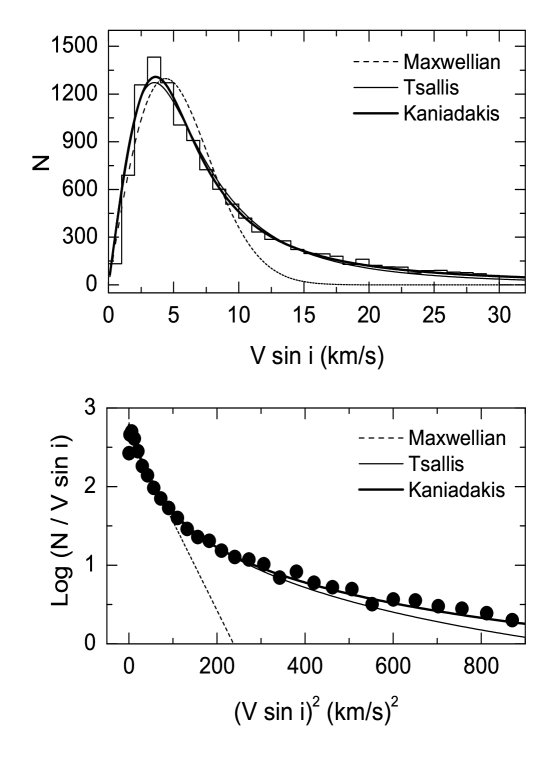
Figure 1: Observed distribution of the rotational velocity for all F and G field stars in the original sample. In the upper panel we show the histogram (number of stars $N$ in each $1~{}km/s$ bin as a function of $V\sin{i}$), whereas in the lower panel, we show the logarithm of $N/V\sin{i}$ as a function of $(V\sin{i})^{2}$. The curves represent the best fitted maxwellian (dashed line), Tsallis (thin line) and Kaniadakis (thick line) distribution. The fitting parameters are in Table 1.

Interestingly, the values of $q$ and $\kappa$ do not change whether we consider the original sample or the complete sample. Nevertheless, the widths of the distributions are notably different. For the original sample $\sigma_{q}=4.25\pm 0.21$ and $\sigma_{\kappa}=4.95\pm 0.15$, while for the complete sample we have $\sigma_{q}=5.08\pm 0.25$ and $\sigma_{\kappa}=5.92\pm 0.19$. Even though the difference is significant, it is within the precision of the projected rotational velocities measurement, that is, $1~{}km/s$.

In the upper panel of Fig. 1 we show the best fits for the histogram of the observed distribution of $V\sin{i}$ according the results in Table 1 for the original sample. The $q$ and $\kappa$-Maxwellian functions are represented, respectively by the thin and thick lines. The dashed line represents the standard Maxwellian function. The distribution of observed $V\sin{i}$ is without a doubt more adequately fitted by either a $q$ and $\kappa$-Maxwellian function. This can be more clearly seen in the lower panel of Fig. 1 where we have plotted the logarithm of the distribution divided by $V\sin{i}$, that is $log(\phi(y)/y)$, as a function of $(V\sin{i})^{2}$ so that the standard Maxwellian is represented by a straight (dashed) line. The Kaniadakis distribution is represented by the thick line while Tsallis distribution by the thin line. We observe that both non-gaussian distributions fit well the observed data, although the Kaniadakis function fits the data slightly better than Tsallis function. This can be seen in Table 1 where the values of the reduced-$\chi^{2}$ is always smaller for the Kaniadakis fit compared with the Tsallis one. Also, the uncertainties in the parameters of the Kaniadakis distribution are smaller than in the case of Tsallis distribution.

In Fig. 2 we present the fitting to the complete sample using the parameter given in Table 1. The results are similar to the original sample. The $q$ and $\kappa$-distribution give the best fit with Kaniadakis function being slightly better.

Finally, we have found no noteworthy difference on the distribution of the projected rotational velocity between single and binary stars (see Table 1). Despite the fact that the values of $q$ and $\sigma_{q}$ and $\kappa$ and $\sigma_{\kappa}$ are slightly larger for binary stars, the difference are, in most case, within the statistical fluctuation.

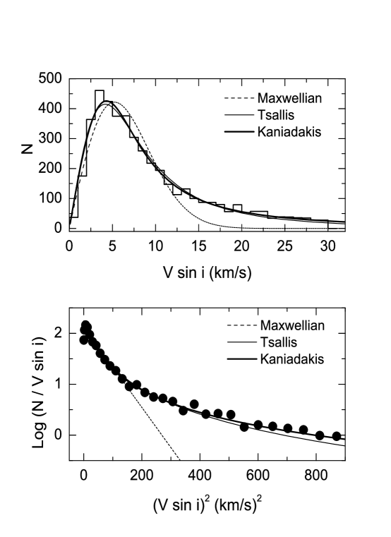
Figure 2: Observed distribution (histogram) of the rotational velocity for all F and G field stars in the complete sample. In the upper panel we show the histogram (number of stars $N$ in each $1~{}km/s$ bin as a function of $V\sin{i}$), whereas in the lower panel, we show the logarithm of $N/V\sin{i}$ as a function of $(V\sin{i})^{2}$. The curves represent the best fitted maxwellian (dashed line), Tsallis (thin line) and Kaniadakis (thick line) distribution. The fitting parameters are in Table 1.

5 Conclusions

In this work we have used non-gaussian statistics to investigate the observed distribution of projected rotational velocity of a magnitude complete sample of more than 16,000 nearby F and G dwarf stars. We have fitted a standard maxwellian and the $q$ and $\kappa$-maxwellian based on the generalization of the power-law statistics proposed by Tsallis and Kaniadakis. We conclude that the $V\sin{i}$ distribution deviates significantly from a standard maxwellian and the best fit is attained for Tsallis distribution with $q=1.521\pm 0.043$ and Kaniadakis distribution with $\kappa=0.667\pm 0.033$. These values correspond to all stars (single + binary) in the complete sample.

As far as we are aware, this is the first time that Tsallis and Kaniadakis statistics are tested for such an exceptionally large sample of stars. This gives us an excellent degree of confidence on the fact that the distribution of stellar rotational velocity does not follow a Maxwellian-Boltzmann law as suggested by the pioneer studies by Chandrasekhar and Munch (1950) and Deutsch (1970). The present results show clearly that for the stellar rotation the non-extensivity holds, and that the distribution of the observed rotational velocity is explained by a generalized power–law statistics in the spirit of Tsallis and Kaniadakis statistical mechanics.

Acknowledgments: The authors are partially supported by the CNPq and FAPERN Brazilian Agencies.

Table 1: Best values of the parameters of Tsallis ($q$ and $\sigma_{q}$) and Kaniadakis ($\kappa$ and $\sigma_{\kappa}$) distribution determined using $\chi^{2}$ test for the rotational velocity of stars in the Nordstr$\ddot{o}$m et al. catalogue.

	N	$q$	$\sigma_{q}$ (km/s)	reduced-$\chi^{2}$	$\kappa$	$\sigma_{\kappa}$ (km/s)	reduced-$\chi^{2}$
Original Sample
all stars	11818	$1.525\pm 0.041$	$4.25\pm 0.21$	4493	$0.667\pm 0.029$	$4.95\pm 0.15$	3088
single	6888	$1.484\pm 0.053$	$4.13\pm 0.25$	422	$0.636\pm 0.038$	$4.74\pm 0.17$	400
binary	4930	$1.551\pm 0.037$	$4.63\pm 0.21$	223	$0.687\pm 0.031$	$5.47\pm 0.17$	207
Complete Sample
all stars	4473	$1.521\pm 0.043$	$5.08\pm 0.25$	550	$0.667\pm 0.033$	$5.92\pm 0.19$	424
single	2382	$1.507\pm 0.046$	$4.92\pm 0.26$	196	$0.655\pm 0.035$	$5.69\pm 0.19$	142
binary	2091	$1.529\pm 0.049$	$5.34\pm 0.31$	149	$0.672\pm 0.041$	$6.26\pm 0.25$	133

References

- (1) Carvalho, J. C., Silva, R., do Nascimento, J. D.Jr., De Medeiros, J. R. 2008, Europhysics Letters, 84, 59001
- (2) Chandrasekhar, S., Munch, G. 1950, ApJ, 111, 142
- (3) De Medeiros, J. R., Da Rocha, C., Mayor, M. 1996, A&A, 314, 499
- (4) Deutsch, A., J. 1970, in: A Slettebak (Ed.), Stellar Rotation, IAU Colloquium, Reidel, Dordrecht, p. 207.
- (5) Dworetssky, M., M. 1974, ApJ, 28, 101
- (6) Gell-Mann, M., and Tsallis C., (Eds.), Nonextensive Entropy - Interdisciplinary Applications, Oxford University Press, New York, (2004).
- (7) Holmberg, J., Nordstrm, B., Andersen, J. 2007, A&A, 475, 519
- (8) Kaniadakis, G. 2002, Phys. Rev. E, 66, 056125
- (9) Kaniadakis, G. 2005, Phys. Rev. E, 72, 036108
- (10) Kraft, R. P. 1970, in Spectroscopic Astrophysics. An Assessment of the Contributions of Otto Struve, G. H. Herbig, ed. (Berkeley: University of California Press), p.385
- (11) Lavagno, A., Kaniadakis, G., Rego-Monteiro, M., Quariti, P., Tsallis, C. 1998, Astrophys. Lett. Commun., 35, 449
- (12) Lapenta, G., Markidis, S., Marocchino, A., and Kaniadakis, G. 2007, ApJ, 666, 949
- (13) Plastino, A., & Plastino, A. R. 1993, Phys. Lett. A, 174, 384
- (14) Nordstrm, B., Mayor, M., Andersen, J., Holmberg, J., Pont, F., Jorgensen, B. R., Olsen, E. H., Udry, S., Mowlavi, N. A. 2004, A&A, 418, 989
- (15) Queloz, D., Allain, S., Mermilliod, J. -C., Bouvier J., Mayor, M. 1998, A&A, 335, 183
- (16) Soares, B. B., Carvalho, J. C., do Nascimento, J. D. Jr. and De Medeiros, J. 2006, Physica A, 364, 413
- (17) Struve, O. 1945, Pop. 53, 202
- (18) Wolff, S. C., Edwards, S., Preston, G. W. 1982, ApJ, 252, 322