Accretion of phantom scalar field into a black hole

Abstract

Using numerical methods we present the first full nonlinear study of phantom scalar field accreted into a black hole. We study different initial configurations and find that the accretion of the field into the black hole can reduce its area down to 50 percent within time scales of the order of few masses of the initial horizon. The analysis includes the cases where the total energy of the space-time is positive or negative. The confirmation of this effect in full nonlinear general relativity implies that the accretion of exotic matter could be considered an evaporation process. We speculate that if this sort of exotic matter has some cosmological significance, this black hole area reduction process might have played a crucial role in black hole formation and population.

The study of black holes in general relativity as thermodynamical systems is an extensive area of research. One of the most interesting features of black holes that can be studied, is the behavior of the area of the horizon during the process of accretion of matter. Assuming that the null energy condition is satisfied, the area of the horizon can only increase HawkingEllis-Book . If this condition is violated then “strange” things can happen, for example, the area of the horizon could decrease and the black hole could shrink. This scenario could be astrophysically and cosmologically interesting if some evidences of exotic matter, violating the null energy condition would be found. For instance, nowadays standard cosmological models, based on observations allow that matter with these types of properties might well play the role of dark energy darkenergy .

In this article we present the accretion of a phantom scalar field into a black hole in the full nonlinear case using numerical methods. The model of phantom scalar field is based on the following Lagrangian density

$${\cal L}={\cal R}+\frac{1}{2}g_{\mu\nu}\partial^{\mu}\phi\partial^{\nu}\phi-V(\phi),$$ (1)

where ${\cal R}$ is the Ricci scalar of the space-time, $g_{\mu\nu}$ is the space-time metric, $\phi$ is the scalar field and $V(\phi)$ its potential, which we choose to be $V(\phi)=\lambda\phi^{2}$ with $\lambda$ a given constant. The difference between the phantom and the standard scalar field is the sign in the kinetic term in the Lagrangian.

When the action constructed with such a Lagrangian density is varied with respect to the metric, the arising Einstein’s equations are related to the stress energy-tensor $T_{\mu\nu}=-\partial_{\mu}\phi\partial_{\nu}\phi-\frac{1}{2}g_{\mu\nu}[-\partial^{\alpha}\phi\partial_{\alpha}\phi+2V]$. Such a stress-energy tensor violates the null energy condition $T_{\mu\nu}k^{\mu}k^{\nu}\leq 0$, where $k^{\mu}$ is a null vector. The immediate implication of this violation is the violation also of the weak energy condition, which in turn implies that observers following timelike trajectories might measure negative energy densities.

The fact that a phantom scalar field violates the null energy condition motivates the study of possible unusual implications in astrophysical scenarios, because the area increasing theorem does not apply in this case HawkingEllis-Book .

Previous experience shows that such a scalar field with $V=0$ is able to produce an area reduction effect, as found during the evolution of wormholes supported by a scalar field that collapse to form black holes whs . Inspired by such an area reduction process we explore in this article the full nonlinear accretion of a phantom scalar field, that is, the case where a nonzero potential is involved.

The evolution equations. We formulate Einstein’s equations coupled to the phantom scalar field in a suitable form for the numerical integration of spherically symmetric black hole solutions. We use geometrized units for which the speed of light and Newton’s constant are equal to one. We write the metric in the general form for the coordinate system $(t,r,\theta,\varphi)$ in spherical coordinates:

$$ds^{2} = -\left(\alpha^{2}-\beta^{r}\beta^{r}\frac{g_{rr}}{\chi}\right)dt^{2}+2\beta^{r}\frac{g_{rr}}{\chi}dtdr$$ (2)

$$+ \frac{1}{\chi}\left[g_{rr}dr^{2}+g_{\theta\theta}(d\theta^{2}+\sin^{2}\theta d\varphi^{2})\right],$$

where $\chi$ acts as a conformal factor relating this metric to a spacelike flat metric, $\beta^{r}$ is the only nonzero component of the shift vector and $\alpha$ is the lapse function.

The procedure used to solve Einstein’s equations is based on a 3+1 decomposition of the space-time and the solution of an initial value problem assuming a puncture type of initial data Bruegmann . In order to follow the evolution of the initial data we found appropriate the use of the Generalized BSSN (GBSSN) evolution system of equations defined previously for spherical symmetry in Brown as opposed to previous successful analyses related to the accretion of a scalar field using Eddington-Finkelstein coordinates under the Arnowitt-Deser-Misner (ADM) formulation that requires excision Thornburg .

The evolution equations in the GBSSN system for the spherically symmetric space-time described by (2) reduce to a set of evolution equations for the conformal factor $\chi$, the conformal metric functions $g_{rr}$ and $g_{\theta\theta}$, the nonzero trace-free part of the conformal extrinsic curvature $A_{rr}$, the trace of the extrinsic curvature $K$ and the contracted conformal Christoffel nonzero symbol $\Gamma^{r}$. The explicit expression for the evolution of these variables can be found in Brown ; BShapiro .

The remaining equations of the geometry involve the evolution of the gauge. For the lapse we choose the 1+$\log$ slicing condition $\partial_{t}\alpha=\beta^{a}\partial_{a}\alpha-2\alpha K$, and for the shift we implemented the recipe for the $\Gamma$-driver condition $\partial_{t}\beta^{a}=\frac{3}{4}B^{a}+\beta^{c}\partial_{c}\beta^{a}$ and $\partial_{t}B^{a}=\partial_{t}\Gamma^{a}+\beta^{c}\partial_{c}B^{a}-\beta^{c}\partial_{c}\Gamma^{a}-\eta B^{a}$, which helps to avoid the slice stretching near the horizon which is known to kill the numerical evolution. In order to avoid instabilities near the puncture we implement a sort of excision without excision using a factor function on the sources of the evolution equations of the form $(r/(1+r))^{4}$ from the coordinate origin out to one quarter of the size of the apparent horizon radius. Even though this function violates the constraints, the convergence tests show that such violation does not propagate outside of the black hole horizon.

The evolution of the scalar field is given by the Klein-Gordon equation

$$\Box\phi=\frac{1}{\sqrt{-g}}\partial_{\mu}[\sqrt{-g}g^{\mu\nu}\partial_{\nu}\phi]=-\partial_{\phi}V,$$ (3)

where $g$ is the determinant of the space-time metric. We solve this equation as a set of two equations for two first-order variables, $\pi=\partial_{t}\phi$ and $\xi=\partial_{r}\phi$, coupled to the evolution of the geometry of the space-time.

Initial data. In order to add the contribution of the scalar field to Einstein’s equations, it is necessary to solve the constraints at the initial time slice which we assume for simplicity to be time-symmetric, which in turn implies that the momentum constraint is identically satisfied. The scalar field contribution consists of a scalar field pulse which is used to solve the Hamiltonian constraint. Another important ingredient is that we set a space-time ansatz similar to that of a Schwarzschild black hole in isotropic coordinates. Thus we assume that the metric at initial time has the form

$$g_{rr}=1,~{}~{}~{}g_{\theta\theta}=r^{2},~{}~{}~{}\chi=\left(1+\frac{M}{2r}+u\right)^{-4},$$ (4)

where $M$ is the ADM mass at the puncture and agrees within numerical precision with the mass of the apparent horizon and $u=u(r,t=0)$ is the function to be determined through the solution of the Hamiltonian constraint. The Hamiltonian constraint in terms of $u$ reads

$$\partial_{rr}u=\frac{1}{8}(\partial_{r}\phi)^{2}\chi^{-1/4}-\frac{2\partial_{r}u}{r}-\frac{V}{4}\chi^{-5/4},$$ (5)

which we solve using an ordinary differential equation integrator. We finally rescale $r$ in such a way that $\chi\rightarrow 1$ when $r\rightarrow\infty$. We notice that with this procedure it is also possible to construct initial data consisting of a large enough amount of scalar field so that the ADM mass could become negative.

It only remains to choose the gauge at initial time, for which we use an initially precollapsed lapse $\alpha=(1+M/2r)^{-2}$, zero shift $\beta^{r}=0$ and zero time derivative $B^{r}=0$. Because the initial time slice has been chosen to be time-symmetric, the extrinsic curvature components are all set to zero initially. These data are used to start up a Cauchy evolution using the GBSSN evolution equations, the gauge conditions and the Klein-Gordon equation.

Numerical methods. The numerical method used to approximate the constraint and evolution equations is a second-order finite differences approximation. We only perform the evolution on a finite domain with artificial boundaries at a finite value of the radial coordinate. The integration in time uses a method of lines with a fourth-order accurate Runge-Kutta time integrator. Throughout the evolution we monitor the Hamiltonian, Momentum and Gamma constraints Brown . We check that they converge with second order to zero as the resolution is increased.

Apparent horizon location. As we are interested in tracking the behavior of the black hole horizon, a useful diagnostics tool is the location of the apparent horizon during the evolution. We locate it from the definition of a marginally trapped surface (MTS) through the condition $\Theta=\nabla_{i}n^{i}+K_{ij}n^{i}n^{j}-K=0$, where $n^{i}$ is an outward pointing unit vector normal to the apparent horizon, $K_{ij}$ are the components of the extrinsic curvature of the spacelike hypersurface on which one calculates the MTSs, and $K$ its trace. The apparent horizon is the outermost MTS. For the metric (2) this equation is written as

$$\Theta = \frac{1}{g_{\theta\theta}\sqrt{\chi g_{rr}}}\left(\chi(\partial_{r}g_{\theta\theta})-g_{\theta\theta}(\partial_{r}\chi)\right)$$ (6)

$$+ 2\left(\frac{A_{rr}}{2g_{rr}}-\frac{1}{3}K\right).$$

In order to track the evolution of the apparent horizon we calculate $\Theta$ at every time step and locate the outermost zero of it at the coordinate radius $r_{AH}$ and calculate the mass of this horizon $M_{AH}=R_{AH}/2$, where $R_{AH}=\sqrt{g_{\theta\theta}/\chi}$ is the areal radius evaluated at $r_{AH}$.

Mass. In order to have an estimate of the space-time mass we use the Misner-Sharp mass defined by MisnerSharp

$$M_{MS} = \frac{R}{2}\left[1+\frac{1}{\alpha^{2}}(\partial_{t}R)^{2}\right.-2\frac{\beta^{r}}{\alpha^{2}}(\partial_{t}R)(\partial_{r}R)$$ (7)

$$- \left.\left(\frac{\chi}{g_{rr}}-\frac{(\beta^{r})^{2}}{\alpha^{2}}\right)(\partial_{r}R)^{2}\right],$$

where $R=\sqrt{g_{\theta\theta}/\chi}$ is the areal radius.

We estimate the ADM mass as $M_{ADM}=\lim_{r\to\infty}M_{MS}$ so that we can estimate the mass of the space-time at any time during the evolution even though we know it should be constant in time.

Null rays and event horizon. We track a bundle of radial outgoing null rays in order to i) approximately locate the event horizon as the surface that separates outgoing null rays that reach spatial infinity from those that do not when launched toward the future and ii) certify that the light-cones point in the correct direction at the apparent and event horizons.

Results. We analyze different cases with various parameters of the initial scalar field profile and different values of $\lambda$ including the case $\lambda=0$ and obtain qualitatively similar results. We use a Gaussian profile or a train of successive Gaussians with different amplitudes and widths for the scalar field. In particular we present two cases characterized by positive and negative ADM masses comentario . In both cases $\lambda=-0.1$; in the case of Lagrangian (1) a negative potential with a maximum is appropriate to keep the scalar field stable. The results are shown in Fig. 1, where we show the evolution of the apparent horizon, Misner-Sharp and ADM masses MisnerSharp . In both cases the area of the apparent horizon decreases and asymptotically in time converges to the Misner-Sharp mass. It is worth noticing that for the case of negative ADM mass we used an initial train of scalar field Gaussians that are being successively accreted, which produces the step-like mass decrease of the horizon mass observed in Fig. 1.

In order to show that the decrease of the black hole area is not a gauge artifact, in Fig. 2 we show a fine-tuned bundle of outgoing null rays for the two cases, and show the approximate location of the event horizon. The fact that the event horizon decreases with the accretion of the scalar field is a strong evidence that the hole area is truly decreasing since the event horizon is a gauge invariant surface unlike the solely consideration of the apparent horizon.

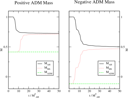
Figure 1: We show the evolution of different masses versus the coordinate time. The solid line represents the mass of the apparent horizon, the dotted line the Misner-Sharp mass extracted at $r\sim 15M^{0}_{AH}$ and the dashed line shows the ADM mass of the space-time. In the left panel the ADM mass of the space-time is positive and in the right one it is negative. In both scenarios the apparent horizon mass decreases and approaches to the Misner-Sharp mass. In the first case the black hole loses approximately $25\%$ of its mass while in the second case it losses almost half of the mass.

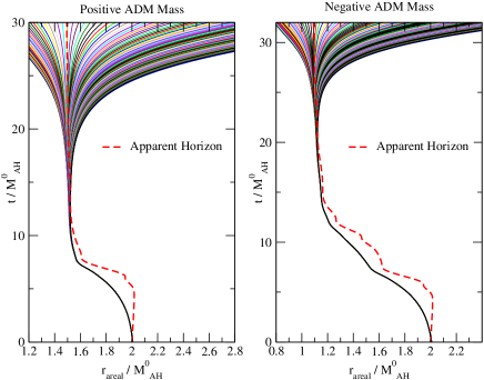
Figure 2: We present a bundle of outgoing null rays showing the approximate location of the event horizon for the runs shown in Fig. 1. It can be seen that this horizon decreases so as the apparent horizon does, showing that our results are not slice dependent. It is interesting to notice that the apparent horizon lies outside the event horizon.

Another interesting result is that the accretion rate and localization of the scalar field depends on the scalar field potential. As an example, in Fig. 3 we compare the behavior of the scalar field in the case where the potential is nonzero with the case of zero potential. In the case of the zero potential the scalar field is quickly accreted whereas in the other case the scalar field gets packed near the horizon and some scalar field is radiated away.

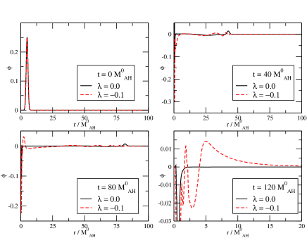
Figure 3: We show snapshots of the scalar field at various times for $\lambda=0$ (continuous line) and $\lambda=-0.1$ (dashed line). The initial profile of the scalar field is the same, although the energy density is slightly different for both cases, nevertheless the time scales are comparable. We point out various effects: i) there is an initial outgoing pulse of scalar field due to the time-symmetry of the initial data in both cases, ii) however in the $\lambda=0$ case the amplitude of the field quickly stabilizes around zero in the domain left behind by the outgoing pulse, whereas the field does not stabilize in the nonzero case, and instead new pulses of the scalar field are being ejected from the region near the horizon.

Finally, in order to validate our results, we have verified the convergence of our results to second order so as the convergence of the violation of the constraints to zero. In Fig. 4 we show the convergence of the $L_{2}$ norm of the constraint violations to zero for the simulations presented in Fig. 1.

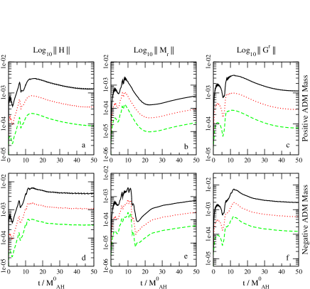
Figure 4: We show the convergence of the $L_{2}$ norm of the violation of the Hamiltonian, momentum and $\Gamma^{r}$ constraints to zero. The plots a,b and c correspond to the simulation with positive ADM mass and the plots d,e and f to the negative ADM mass case.

Discussion. In order to illustrate the process we consider the hypothetical case of a black hole space-time with positive ADM mass. Assuming the mass of the original black hole apparent horizon is $M_{phys}=10^{9}M_{\odot}$, and that a pulse of scalar field with amplitude $0.25$ is accreted, the time-scale for the field to reduce the mass of the hole in 25% is $t\sim 1$day in coordinate time (see the results in Fig. 1).

In theory, due to the fact that our results scale with the initial mass of the black hole, it would always be possible to construct the appropriate scalar field profile so that the process of accretion could be iterated reducing half of the mass of the horizon each time.

The results presented constitute solid steps toward exploring the accretion of phantom scalar field dark energy under different astrophysical conditions, mainly those related to cosmologically motivated potentials and wavelengths of the scalar field darkenergy . It would also be interesting to investigate the full nonlinear accretion of phantom energy in black holes immersed in a FRW geometry like those in Mc Vittie-type black hole solutions Faraoni2007 , because these scenarios could have cosmologically interesting implications.

One of the properties of this type of field in the cosmological scenario is that if $T_{\mu\nu}$ is the stress-energy tensor, the ratio between the radial pressure $p_{r}=n^{\mu}T_{\mu r}$ and the energy density $\rho=n^{\mu}n^{\nu}T_{\mu\nu}$ measured by Eulerian observers with $n^{\mu}$ the normal to the spatial hypersurfaces, provides an equation of state such that $\omega_{r}=\frac{p_{r}}{\rho}<-1$ in the case of nonzero potential, and $\omega_{r}=1$ in the case of zero potential. These properties change when the configurations depend on the spatial coordinates and the potential is nonzero. For instance, in the case discussed here, the scalar field depends on the spatial coordinate and there are regions where the equation of state $\omega<-1$ is satisfied, however there are also regions where $\phi$ approaches zero and the potential becomes zero too, in which case the scalar field would behave as stiff matter $\omega=1$.

These results should imply important restrictions on the parameters of phantom dark energy models related to the abundance and mass of black holes and the abundance and lifetime of PBHs for instance. We also expect that the type of process shown in this article competes with other horizon-reducing processes of black holes.

A detailed study containing various initial conditions, more violent horizon-shrinking processes, dynamical properties of horizons and the study of the possibility of producing a naked the singularity is in progress detailedpaper .

- (1) S.W. Hawking and G.F.R. Ellis, The Large Scale Structure of Space Time, Cambridge University Press, 1973.
- (2) Kowalski et al., Astrophys.J.686:749-778,2008.
- (3) J. A. González, F. S. Guzmán, O. Sarbach, Class. Quantum Grav. 26:015011, 2009. E-print: arXiv:0806.1370 [gr-qc].
- (4) S. Brandt and B. Bruegmann, Phys. Rev. Lett. 78:3606-3609, 1997
- (5) J. D. Brown, Class. Quantum Grav., 25:205004, 2008.
- (6) J. Thornburg, Phys. Rev. D 59:104007, 1999. Ibid. arXiv:gr-qc/9906022.
- (7) T. Baumgarte and S. L. Shapiro, Phys. Rev. D 59:024007 (1998).
- (8) C.W. Misner and D.H. Sharp, Phys. Rev. 136:B571–B576, 1964.
- (9) It is not surprising that it is possible to construct space-times with negative ADM mass because the contribution of the scalar field to the energy density is negative.
- (10) V. Faraoni, and A. Jacques, Phys. Rev. D 76:063510, 2007.
- (11) F. Lora, J. A. González, F. S. Guzmán, O Sarbach, et al. in progress.