Integral field spectroscopy with SINFONI of VVDS galaxies

Abstract

Context. Identifying the main processes of galaxy assembly at high redshifts is still a major issue to understand galaxy formation and evolution at early epochs in the history of the Universe.

Aims. This work aims to provide a first insight into the dynamics and mass assembly of galaxies at redshifts $1.2<z<1.6$, the early epoch just before the sharp decrease of the cosmic star formation rate.

Methods. We use the near-infrared integral field spectrograph SINFONI on the ESO-VLT under 0.65″ seeing to obtain spatially resolved spectroscopy on nine emission line galaxies with $1.2\leq z\leq 1.6$ from the VIMOS VLT Deep Survey. We derive the velocity fields and velocity dispersions on kpc scales using the H$\alpha$ emission line.

Results. Out of the nine star-forming galaxies, we find that galaxies distribute in three groups: two galaxies can be well reproduced by a rotating disk, three systems can be classified as major mergers and four galaxies show disturbed dynamics and high velocity dispersion. We argue that there is evidence for hierarchical mass assembly from major merger, with most massive galaxies with $M>10^{11}\,{\rm M_{\odot}}$ subject to at least one major merger over a 3 Gyr period as well as for continuous accretion feeding strong star formation.

Conclusions. These results point towards a galaxy formation and assembly scenario which involves several processes, possibly acting in parallel, with major mergers and continuous gas accretion playing a major role. Well controlled samples representative of the bulk of the galaxy population at this key cosmic time are necessary to make further progress.

1 Introduction

In the current paradigm, galaxies are formed in dark matter haloes which grow along cosmic time via hierarchical assembly of smaller units. While in this picture halo-halo merging is the main physical process driving the assembly of dark matter haloes, it is unclear how this merging process directly affects the build-up of galaxies, and how other physical processes play a role.

Considerable efforts have been invested to understand galaxy evolution in the past two decades. We now have a global, but as yet incomplete, picture of the evolution of the parameters describing the main galaxy population, with e.g. the global star formation rate reaching a peak at redshifts 1 to 2.5 (e.g. Tresse et al., 2007; Hopkins & Beacom, 2006). A clear result now emerging is that early type galaxies have experienced a major growth in stellar mass density from a redshift $z\sim 2$ to $z\sim 1$, while late-type galaxies have been growing their stellar mass more slowly in this period (e.g. Arnouts et al., 2007; Bundy et al., 2005). It is also claimed that galaxy evolution proceeds via a downsizing scenario, whereby the most massive galaxies assemble their mass first (Cowie et al., 1996).

However, much remains to be done to understand how galaxies of different types have been built along cosmic time. Several key questions are still subject to considerable debate: (i) How were galaxies assembled in details? (ii) When and at what rate did galaxies of different masses form? (iii) What is the connection between bulge and disk formation? (iv) What is the link between the various high-z galaxy populations, their origin and their subsequent fates? (v) What is the connection between star formation and the AGN phenomenon ?

Several physical processes have been identified to be contributing to the evolution of galaxies, but their relative contributions, main epoch of action, and associated timescales, remain poorly constrained. Merging is identified as an important contributor through direct evidence of on-going events, or indirect fossil remnants (e.g. Conselice et al., 2003; Lotz et al., 2008), and the merger rate and its evolution is now demonstrated to be strongly dependent on the luminosity or stellar mass of the galaxies involved (e.g. de Ravel et al., 2009). In addition, the effect of the competing processes of cooling, angular momentum exchange, feedback from star formation and AGNs, or gas accretion, are to be further investigated (Somerville et al., 2008).

Until recently, the favoured picture was that the star formation and stellar mass assembly of massive galaxies was a direct consequence of major merging events at early cosmic epochs (Glazebrook et al., 2004). However, recent observations of individual galaxies have revealed that large and massive disks with strong star formation seem to be already in place at redshifts $z\sim 2$, without apparent signs for major merging events (Förster Schreiber et al., 2006; Wright et al., 2007, 2009; Law et al., 2007, 2009; Genzel et al., 2006, 2008). This has led to suggest that the majority of star forming galaxies is fed by gas via cold flows along streams of the cosmic web (including minor merger), continuously fueling the star formation (Dekel et al., 2009). This scenario is further supported by the tight correlation between stellar mass and star formation rate in high redshift star forming galaxies (e.g. Daddi et al., 2007; Noeske et al., 2007; Elbaz et al., 2007). Dynamical processes internal to galaxies can then drive secular evolution of disks and the formation of bulges and spheroids.

The detailed knowledge of the kinematics of a galaxy on kiloparsec scales is needed to identify its dynamical state (disk in rotation, spheroid, major marger event or more complex kinematics). The integral field technique enables one to compute accurate total dynamical masses, to trace the spatial distribution of stars and gas, as well as to evaluate the contribution of stellar populations including stellar initial mass function (IMF), or gas metallicity. The velocity field of spiral/disk galaxies, can be used to put important constraints on total masses and hence on dark matter halo masses, thought to be an important driver of galaxy evolution.

At low redshifts, the knowledge of 2D velocity fields has proved to be a powerful kinematical tool to investigate the properties of nearby galaxies (Östlin et al., 2001; Veilleux et al., 2001; Swinbank et al., 2003; Mendes de Oliveira et al., 2003; Garrido et al., 2004; Epinat et al., 2008a, b). The velocity fields of galaxies at intermediate redshift ($0.4<z<0.75$) have been investigated using FLAMES/GIRAFFE at VLT (Flores et al., 2006; Puech et al., 2006; Yang et al., 2008; Neichel et al., 2008; Puech et al., 2008). In their sample of 65 galaxies, Yang et al. (2008) found about 32% of relaxed rotating disks. These rotating disks produce a Tully-Fisher relation (Tully & Fisher, 1977) which has apparently not evolved in slope and scatter since z=0.6. They however detect an evolution of the K-band Tully-Fisher relation zero point that, if interpreted as an evolution of the K-band luminosity, would imply a brightening of 0.66$\pm$0.14 mag between $z\sim 0.6$ and $z=0$. They suggest that the large scatter found in previously reported Tully-Fisher relations at moderate redshifts are produced by the numerous (65%) galaxies with perturbed or complex kinematics.

At higher redshifts the SINS survey has pioneered the detailed observations of galaxies at $z\sim 2$ (Förster Schreiber et al., 2006; Genzel et al., 2006, 2008; Shapiro et al., 2008; Cresci et al., 2009), demonstrating that near infrared integral field spectroscopy is the best tool to securely measure the kinematical properties at high redshifts $z>1$. These authors have found that galaxies have an extremely large velocity dispersion ($\sigma\sim 80$ $km\leavevmode\nobreak\ s^{-1}$) as compared to their rotational velocity. They favor the hypothesis of early buildup of central disks and bulges by secular evolution in gas-rich disks. Fast turbulent speeds in the gaseous component imply the formation of massive clumps. Gas-rich primordial disks may evolve through a clumpy phase into bright early-type disk galaxies with a massive exponential disk, a classical bulge and possibly a central black hole (Noguchi, 1999; Immeli et al., 2004a, b; Elmegreen et al., 2005; Bournaud et al., 2007, 2008). These massive clumps are suggested from NACO high resolution deep imaging and H$\alpha$ maps from adaptive optics SINFONI observation in two galaxies of the SINS sample (Genzel et al., 2008).

The number of galaxies observed at or around the peak in star-formation at $z\sim 1-2.5$ is still relatively small, and detailed observations of a large volume complete sample of galaxies selected from an homogeneous set of selection criteria are needed to clarify the respective contributions of merging and continuous gas feed by accretion.

Assembling large samples of galaxies is not an easy task as we need to extract from large spectroscopic surveys, selected with well controlled criteria, those galaxies with accurate spectroscopic redshifts for which the H$\alpha$ line emission falls outside bright OH sky lines. The VVDS (Le Fèvre et al., 2005) survey has been designed to map the evolution of galaxies, large scale structures and AGNs from the spectroscopic redshift measurement of tens of thousands of objects. This dedicated program has successfully crossed the “redshift desert” $1<z<3$, providing for the first time a complete magnitude-limited sample of $\sim 800$ galaxy redshifts in the “Ultra-deep” ($I_{AB}\leq 24.75$) sample (Le Fèvre et al., in preparation), $\sim$ 11 000 galaxy redshifts in the “deep” ($I_{AB}\leq 24$) sample (Le Fèvre et al., 2005), and $\sim$ 40 000 in the “wide” ($I_{AB}\leq 22.5$) sample (Garilli et al., 2008).

We are using VVDS to select targets for a large observing program at the ESO-VLT aimed at probing the mass assembly and metallicity evolution of a representative sample of galaxies at $1<z<2$, a crucial epoch corresponding to the peak of cosmic star formation activity. The main goal of the MASSIV (Mass Assembly Survey with SINFONI in VVDS) project is to obtain a detailed description of the mix of dynamical types at this epoch and to follow the evolution of fundamental scaling relations, such as the Tully-Fisher or the mass-metallicity relations, and therefore constrain galaxy evolution scenarios.

In this paper we present the first results obtained by MASSIV focusing on the kinematics of nine galaxies with $1.2\leq z\leq 1.6$ observed during the MASSIV pilot program. A companion paper (Queyrel et al., 2009) is devoted to the mass-metallicity relation of galaxies at these redshifts using the same data. In (§2) we describe our observations and data reductions. In (§3) we present the morphological, physical, kinematical and dynamical measurements of the galaxies of our sample. In (§4 ) we classify the galaxies exploiting the full kinematical information and discuss the Tully-Fisher relation. Our discussion and conclusions are provided in (§5). Appendix A contains detailed individual comments for each galaxy. We assume a cosmology with $\Omega_{m}=0.3$, $\Omega_{\Lambda}=0.7$ and $H_{0}$ = 70  km s^-1 Mpc^-1  throughout.

2 Data and Observations

2.1 Sample selection

Figure 1: Selection of late-type $1<z<1.54$ star-forming galaxies with secure redshift and measured [O ii] $\lambda$3727Å emission line in the VVDS-22h ($I_{\rm AB}\leq 22.5$, small triangles) and VVDS-02h ($I_{\rm AB}\leq 24$, small squares) fields for SINFONI follow-up observations. Among these galaxies we selected those showing the strongest [O ii] $\lambda$3727Å emission line (filled symbols: EW $>50$ Å and flux $>5\times 10^{-17}$ erg s^-1cm^-2, measured on VIMOS spectra) for H$\alpha$ to be easily detected in the near-IR. The nine galaxies studied in this paper are indicated as large blue triangles (VVDS-22h field) and large red squares (VVDS-02h field).

Table 1: Table of observations

VVDS ID	$\alpha$	$\delta$	z	$I_{\rm AB}$	Field	texp	Seeing	Run ID
	J2000	J2000		mag		hours	″
(1)	(2)	(3)	(4)	(5)	(6)	(7)	(8)	(9)
020116027	02:25:51.133	-04:45:04.48	1.5259	22.875	VVDS-02h	1.67	0.65	075.A-0318(A)
020182331	02:26:44.260	-04:35:51.89	1.2286	22.729	VVDS-02h	3	0.72	078.A-0177(A)
020147106	02:26:45.386	-04:40:47.39	1.5174	22.502	VVDS-02h	2	0.74	075.A-0318(A)
020261328	02:27:11.049	-04:25:31.60	1.5291	23.897	VVDS-02h	1	0.61	075.A-0318(A)
220596913	22:14:29.184	+00:22:18.89	1.2667	21.841	VVDS-22h	1.75	0.47	075.A-0318(A)
220584167	22:15:23.038	+00:18:47.01	1.4637	22.036	VVDS-22h	1.75	0.74	075.A-0318(A)
220544103	22:15:25.708	+00:06:39.53	1.3970	22.469	VVDS-22h	1	0.69	075.A-0318(A)
220015726	22:15:42.455	+00:29:03.59	1.3091	22.473	VVDS-22h	2	0.58	075.A-0318(A)
220014252	22:17:45.690	+00:28:39.47	1.3097	22.101	VVDS-22h	2	0.70	075.A-0318(A)

(1) Source VVDS identification number, (2) and (3) Coordinates, (4) VVDS spectroscopic redshift, (5) AB magnitude in I-band, (6) VVDS-22h wide field ($17.5\leq I_{\rm AB}\leq 22.5$) and VVDS-02h deep field ($17.5\leq I_{\rm AB}\leq 24.0$), (7) Exposure time, (8) Median seeing of SINFONI observations measured on PSF stars, (9) ESO program.

We have used the VIMOS VLT Deep Survey sample to select galaxies with known spectroscopic redshifts across the peak of star formation activity. The VVDS is a complete magnitude selected sample avoiding the biases linked to a priori color selection techniques. This sample offers the advantage of combining a large sample with a robust selection function and secure spectroscopic redshifts. The latter are necessary to engage into long single objects integrations with SINFONI (Eisenhauer et al., 2003; Bonnet et al., 2004) being sure to observe the H$\alpha$ line outside bright OH night-sky emission lines.

From the existing VVDS dataset, we have available today a unique sample of more than 1500 galaxies in the redshift domain $1<z<2$ with accurate (to the fourth digit) and secure spectroscopic redshifts (confidence level $>$ 90%; Le Fèvre et al., 2005). This sample being purely $I$-band limited, it contains both star-forming and passive galaxies distributed over a wide range of stellar masses, enabling to easily define volume limited sub-samples. For the MASSIV program, we have defined a sample of $\sim$ 140 VVDS star-forming galaxies at $1.0<z<1.8$ suitable for SINFONI observations. In most of the cases, the galaxies are selected on the basis of their measured intensity of [O ii] $\lambda$3727 emission line in the VIMOS spectrum or, for a few cases, on their observed photometric $UBVRIK$ spectral energy distribution which is typical of star-forming galaxies. The star formation criteria ensure that the brightest rest-frame optical emission lines, mainly H$\alpha$, [O iii] $\lambda\lambda$4959,5007, [N ii] $\lambda$6584 used to probe kinematics and chemical abundances, will be observed with SINFONI in the NIR bands.

For the pilot observations presented in this paper, the selection has been made on [O ii] $\lambda$3727 emission line only thus restricting the redshift range to $1<z<1.54$. We have selected galaxies showing the strongest [O ii] $\lambda$3727 emission line (EW $>50$ Å and flux $>5\times 10^{-17}$ erg s^-1cm^-2) as measured on VIMOS spectra (see Figure 1) for H$\alpha$ to be easily detected in the near-IR. Among these candidates, we have further restricted the sample taking into account one important observational constraint: the observed wavelength of H$\alpha$ line had to fall at least 10Å away from strong OH night-sky lines, to avoid heavy contamination of the galaxy spectrum by sky subtraction residuals. Among the remaining list of promising candidates, we have randomly picked up twelve galaxies to carry out these first pilot observations. These criteria for selecting late-type star-forming galaxies have been shown to be very efficient. For the first observing runs, our success rate of selection has been around 85%: 9 galaxies over 12 observed show strong rest-frame optical emission lines in SINFONI datacubes, the 3 remaining show a signal too faint to derive reliable velocity maps. Among the nine VVDS star-forming galaxies, five have been selected in the VVDS-22h ($17.5\leq I_{\rm AB}\leq 22.5$) field and four in the VVDS-02h ($17.5\leq I_{\rm AB}\leq 24.0$) field. These targets span a redshift range between $z\sim 1.22$ and $z\sim 1.53$ (see Table 1).

Table 2: Fluxes and luminosities of VVDS galaxies

VVDS ID	UAB	L1500	F(H$\alpha$)	L(H$\alpha$)	F([O ii])	L([O ii])
	mag	$10^{+28}$ ergs s-1 Hz-1	$10^{-17}$ ergs s-1 cm-2	$10^{+41}$ ergs s-1	$10^{-17}$ ergs s-1 cm-2	$10^{+41}$ ergs s-1
(1)	(2)	(3)	(4)	(5)	(6)	(7)
020116027	24.0	5.1 $\pm$ 0.2	6 $\pm$ 1	9 $\pm$ 2	6 $\pm$ 2	9 $\pm$ 2
020182331	24.1	3.7 $\pm$ 0.1	55 $\pm$ 14	47 $\pm$ 13	20 $\pm$ 2	17 $\pm$ 2
020147106	23.4	12.9 $\pm$ 0.1	22 $\pm$ 6	32 $\pm$ 9	9 $\pm$ 2	12 $\pm$ 3
020261328	24.2	4.4 $\pm$ 0.2	5 $\pm$ 1	7 $\pm$ 2	10 $\pm$ 2	15 $\pm$ 3
220596913	23.1	8.7 $\pm$ 0.4	33 $\pm$ 6	32 $\pm$ 6	19 $\pm$ 2	17 $\pm$ 2
220584167	22.9	12.5 $\pm$ 0.6	48 $\pm$ 10	64 $\pm$ 14	18 $\pm$ 2	24 $\pm$ 3
220544103	23.3	9.4 $\pm$ 0.5	161 $\pm$ 29	192 $\pm$ 35	25 $\pm$ 3	30 $\pm$ 4
220015726	24.0	3.1 $\pm$ 0.4	26 $\pm$ 3	26 $\pm$ 3	9 $\pm$ 2	10 $\pm$ 2
220014252	22.7	11.2 $\pm$ 0.3	212 $\pm$ 27	216 $\pm$ 28	38 $\pm$ 2	38 $\pm$ 2

(1) Source VVDS identification number, (2) AB magnitude in $U$-band, (3) UV luminosity, (4) SINFONI H$\alpha$ flux, (5) H$\alpha$ luminosity, (6) VIMOS [O ii] $\lambda$3727 flux, (7) [O ii] $\lambda$3727 luminosity.

Table 3: SFRs and extinctions of VVDS galaxies

VVDS ID	SFRUV	SFRHα	SFR${}_{\textup{\scriptsize{[O\,{\sc ii}]}}}$	SFRSED	$E(B-V)_{UV/H\alpha}$	$E(B-V)_{SED}$
	M⊙ yr-1	M⊙ yr-1	M⊙ yr-1	M⊙ yr-1	mag	mag
(1)	(2)	(3)	(4)	(5)	(6)	(7)
020116027	7.2 $\pm$ 0.3	7 $\pm$ 2	13 $\pm$ 4	46 ${}^{+28}_{-21}$	0.0	0.2
020182331	5.2 $\pm$ 0.2	38 $\pm$ 10	24 $\pm$ 7	67 ${}^{+3}_{-25}$	0.2	0.3
020147106	18.1 $\pm$ 0.2	25 $\pm$ 7	17 $\pm$ 6	55 ${}^{+6}_{-2}$	0.0	0.1
020261328	6.2 $\pm$ 0.2	6 $\pm$ 2	21 $\pm$ 7	8 ${}^{+23}_{-5}$	0.0	0.1
220596913	12.1 $\pm$ 0.6	24 $\pm$ 5	24 $\pm$ 7	77 ${}^{+109}_{-29}$	0.1	0.1
220584167	17.5 $\pm$ 0.8	51 $\pm$ 11	34 $\pm$ 10	158 ${}^{+113}_{-92}$	0.1	0.3
220544103	13.2 $\pm$ 0.7	152 $\pm$ 28	42 $\pm$ 13	46 ${}^{+73}_{-15}$	0.3	0.3
220015726	4.3 $\pm$ 0.5	21 $\pm$ 3	13 $\pm$ 4	86 ${}^{+39}_{-32}$	0.2	0.2
220014252	15.7 $\pm$ 0.4	171 $\pm$ 22	54 $\pm$ 16	84 ${}^{+121}_{-48}$	0.3	0.3

(1) Source VVDS identification number, SFRs deduced respectively from (2) UV flux, (3) H$\alpha$ flux, (4) [O ii] $\lambda$3727 flux and (5) SEDs, Reddening suffered by the ionised gas respectively computed (6) from the UV/H$\alpha$ ratio and (7) from SED modeling.

2.2 SINFONI observations and data reduction

The NIR spectroscopic observations were obtained with the 3D-spectrograph SINFONI at ESO-VLT during two four-nights runs, on September 5-8, 2005 (ESO run 75.A-0318) and on November 12-15, 2006 (ESO run 78.A-0177). SINFONI was used in its seeing-limited mode, with the 0.125″$\times$0.25″ pixel scale leading to a field-of-view of 8″$\times$8″, and the H grism providing a spectral resolution $R\sim 4000$. Conditions were not photometric and the mean seeing measured on PSF stars was around 0.65″ (see details in Table 1). The PSF stars were observed by SINFONI in $H$-band for each pointing on any target. Each target was acquired through a blind offset from a nearby bright star. Each observation was obtained by nodding the position of the galaxy within the 8″ $\times$ 8″ SINFONI field-of-view, generally by locating the source in two opposite corners. This observational procedure allows background subtraction by using frames contiguous in time, but with the galaxy in different locations. Moreover, the target was never located exactly at the same position on the detector, a minimal dithering of 0.3″ was required in order to minimize instrumental artifacts when the individual observations are aligned and combined together. The total on-source integration times are listed in Table 1 and range between 1 and 3 hours. As observations were performed in visitor mode, the integration time has been adjusted on the fly depending on the signal to noise achieved for the H$\alpha$ emission line.

Data reduction has been performed with the ESO-SINFONI pipeline (version 1.7.1, see Abuter et al., 2006; Modigliani et al., 2007). The pipeline subtracts the sky background from the temporally contiguous frames, flat-fields images, spectrally calibrates each individual observation and then reconstructs the datacube. Individual cubes were aligned in the spatial direction by relying on the telescope offsets from a nearby bright star and then combined together. A flux calibration is mandatory in order to derive absolute parameters (e.g. star formation rate) from the flux measured in emission lines. To this end, each science observation has been immediately followed by the observation of a telluric standard star.

3 Measurements

3.1 Stellar masses, star formation rates and extinction

Figure 2: Best SED fit model BC03 (continuous line) and photometric points overplotted for the nine galaxies of the sample.

Stellar mass $M_{star}$ and star formation rate (SFR) estimates for our sample were obtained using the GOSSIP spectral energy distribution (SED) modeling software (Franzetti et al., 2008). We used as input for the SED fitting the multi-band photometric observations available in VVDS fields, including $BVRI$ data from the CFHT, $UBVRZs$ data from the CFHT Legacy Survey, $J$- and $K$-bands data from SOFI at the NTT and from the UKIDSS survey, and the VVDS-Deep spectra. The photometric and spectroscopic data were fitted with a grid of stellar population models, generated using the BC03 population synthesis code (Bruzual & Charlot, 2003), assuming a set of “delayed” star formation histories (see Gavazzi et al., 2002 for details), a Salpeter (1955) IMF with lower and upper mass cutoffs of respectively 0.1 and 100 $\,{\rm M_{\odot}}$, a metallicity ranging from 0.02 and 2.5 solar metallicity and a Large Magellanic Cloud reddening law (Pei, 1992) with an extinction $E(B-V)$ ranging from 0 to 0.3. The parameters for the best-fitting model for each galaxy are taken as the best fitting values for both the galaxy stellar mass and SFR. On top of the best fitting values, GOSSIP computes also the Probability Distribution Function (PDF), following the method described in Walcher et al. (2008). The median of the PDF and its confidence regions are then used to derive a robust estimate of value and error for the parameter that is to be determined. Stellar masses for the galaxies of this paper are reported in Table LABEL:table_mass. The best SED fit model for each galaxy is presented in Figure 2.

In addition to the determination from the SED fitting (SFR_SED), SFRs for the nine star-forming galaxies in our sample can be deduced from the H$\alpha$ (SFR_Hα) flux, from the [O ii] $\lambda$3727 flux (SFR${}_{\textup{\scriptsize{[O\,{\sc ii}]}}}$) and from the rest-frame UV continuum emission (SFR_UV). As these four estimators are affected differently by dust and star formation history, our results can in principle tell us about the extinction and stellar populations of the galaxies.

The H$\alpha$ recombination line is a direct probe of the young, massive stellar population and therefore provides a nearly instantaneous (i.e. averaged on the last ten million years) measure of the SFR. Moreover, the H$\alpha$ line is less affected by dust extinction compared to e.g. UV estimators. We have calculated SFR_Hα following Kennicutt (1998):

$$\frac{\textup{SFR}_{\mathrm{H}\alpha}}{[\,{\rm M_{\odot}}\textup{ yr}^{-1}]}=7.9\times 10^{-42}\frac{\textup{L}(\mathrm{H}\alpha)}{[\textup{erg s}^{-1}]}$$ (1)

where the H$\alpha$ luminosity $\textup{L}(\mathrm{H}\alpha)$ has been derived from the H$\alpha$ flux measured on SINFONI data by Queyrel et al. (2009).

The [O ii] $\lambda$3727 emission line luminosity L([O ii]) is not directly coupled to the ionising luminosity and its excitation is sensitive to abundance and the ionization state of the gas. It can however be empirically used as a quantitative SFR tracer. We have computed SFR${}_{\textup{\scriptsize{[O\,{\sc ii}]}}}$ following the calibration provided by Kennicutt (1998):

$$\frac{\textup{SFR}_{\textup{\scriptsize{[O\,{\sc ii}]}}}}{[\,{\rm M_{\odot}}\textup{ yr}^{-1}]}=(1.4\pm 0.4)\times 10^{-41}\frac{\textup{L([O\,{\sc ii}])}}{[\textup{erg s}^{-1}]}$$ (2)

where L([O ii]) has been derived from the [O ii] $\lambda$3727 flux measured on VIMOS spectra.

Ultraviolet-derived SFRs were calculated from the broadband optical photometry. Given the redshifts of our targets, optical photometry provides indeed an information on the amount of rest-frame UV flux. The UV continuum around 1500 Å is roughly flat if the flux is expressed in frequency units. The mean luminosity inside the optical broad-band filter which corresponds to the rest-frame 1500 Å continuum L₁₅₀₀, at the given redshift $z$ of the source, is thus a very good approximation of the level of this continuum. The mean luminosity in frequency units is calculated following this equation:

$$\frac{\textup{L}_{1500}}{[\textup{erg\leavevmode\nobreak\ s${}^{-1}$\leavevmode\nobreak\ Hz${}^{-1}$}]}=10^{-0.4\leavevmode\nobreak\ U_{AB}-23}\times 3631\times 4\pi\frac{\left(\frac{D_{L}}{[\textup{cm}]}\right)^{2}}{1+z}$$ (3)

$D_{L}$ beeing the luminous distance.

We have then deduced SFR_UV following Kennicutt (1998):

$$\frac{\textup{SFR}_{UV}}{[\,{\rm M_{\odot}}\textup{ yr}^{-1}]}=1.4\times 10^{-28}\leavevmode\nobreak\ \frac{\textup{L}_{1500}}{[\textup{erg\leavevmode\nobreak\ s${}^{-1}$\leavevmode\nobreak\ Hz${}^{-1}$}]}$$ (4)

The three equations 1, 2 and 4 assume a Salpeter IMF with lower and upper mass cutoffs of 0.1 and 100 $\,{\rm M_{\odot}}$ and do not include any effects of attenuation by dust.

Table 2 gives the AB magnitude in $U$-band, UV flux, H$\alpha$ and [O ii] $\lambda$3727 fluxes and luminosities used to compute the four SFRs stored in Table 3 together with the reddening values deduced from SED fitting and from the UV/H$\alpha$ SFR ratio.

The UV SFR may be much more strongly affected by extinction than the H$\alpha$ one due to a shorter wavelength emission. Its comparison with the H$\alpha$ SFR may thus provide an estimate of the amount of dust. Assuming that all of the ionizing photons are reprocessed into lines, therefore $\textup{SFR}_{\mathrm{H}\alpha}=\textup{SFR}_{UV}$, we thus computed the interstellar gas extinction ($E(B-V)$) using the intrinsic starburst flux density $f_{i}(\lambda)$ via:

$$f_{i}(\lambda)=f_{o}(\lambda)\leavevmode\nobreak\ 10^{0.4\leavevmode\nobreak\ E(B-V)\leavevmode\nobreak\ k^{e}(\lambda)}\leavevmode\nobreak\ ,$$ (5)

where the obscuration curve for the stellar continuum, $k^{e}(\lambda)$, is given by Calzetti et al. (2000) for star-forming galaxies:

$$k^{e}(\lambda)=1.17\times(-2.156+1.509/\lambda-0.198/\lambda^{2}+0.011/\lambda^{3})+1.78$$

$$\textup{for\leavevmode\nobreak\ \leavevmode\nobreak\ \leavevmode\nobreak\ }0.12\mu m\leq\lambda<0.63\mu m$$ (6)

The amount of interstellar extinction estimated in our sample (mean value $E(B-V)\sim 0.15$) is typical of star-forming galaxies in the local and intermediate-redshift universe and is in very good agreement with the reddening values derived at similar redshifts in UV-selected galaxy samples by Erb et al. (2006). Figure 3 shows a good agreement between extinctions derived from SED fitting and from the UV/H$\alpha$ SFR ratio. However, the SFR-based extinctions are systematically underestimated compared to the SED ones. This may be due to the uncertainties in the absolute flux calibration both in the rest-frame UV and even more important in the SINFONI data.

In Figure 4 (left), we compare the SFR derived from [O ii] and H$\alpha$ emission lines. The agreement is good taking into account that neither H$\alpha$ nor [O ii] flux has been corrected for reddening. Indeed, H$\alpha$ based SFR are systematically higher than [O ii] ones because [O ii] is more affected by extinction than H$\alpha$, except for the two galaxies with almost no extinction (see Table 3). The fact that the two galaxies with the highest extinction ($E(B-V)\sim 0.3$) show the largest deviation is supporting this interpretation.

The SFR deduced from the SED fitting (SFR_SED) provides an internal correction for dust extinction but is averaged on a timescale ten times longer than the SFR derived from H$\alpha$. The comparison between these two SFRs may provide information on the ratio between recent and older star formation activity, and thus can give an hint on the presence of recent bursts (see Figure 4, right). Despite the large uncertainties inherent to the SED-based SFR determination, a good agreement between the two SFR estimators is seen for the three galaxies classified as perturbed rotators (see section 4.1) with a H$\alpha$-based SFR value lower than $50$ M_⊙ yr^-1. The two galaxies classified as rotating disks and the two merging systems VVDS020116027 and VVDS220596913 show an instantaneous H$\alpha$-based SFR (timescale $\sim 10$ Myr) which is lower (by a factor 2-4) than the SED-based SFR integrated over a longer timescale (a few hundreds Myr). On the contrary, the two galaxies with the highest values of H$\alpha$-based SFR ($>150$ M_⊙ yr^-1, VVDS220544103 and VVDS220014252) are typical starburst galaxies with a high ratio between the instantaneous and integrated SFRs.

Figure 3: Comparison of extinctions computed from SED fitting (x-axis) and from the comparison of SFRs deduced from UV and H$\alpha$ luminosities (y-axis). The dashed line indicates $y=x$.

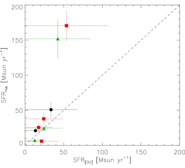
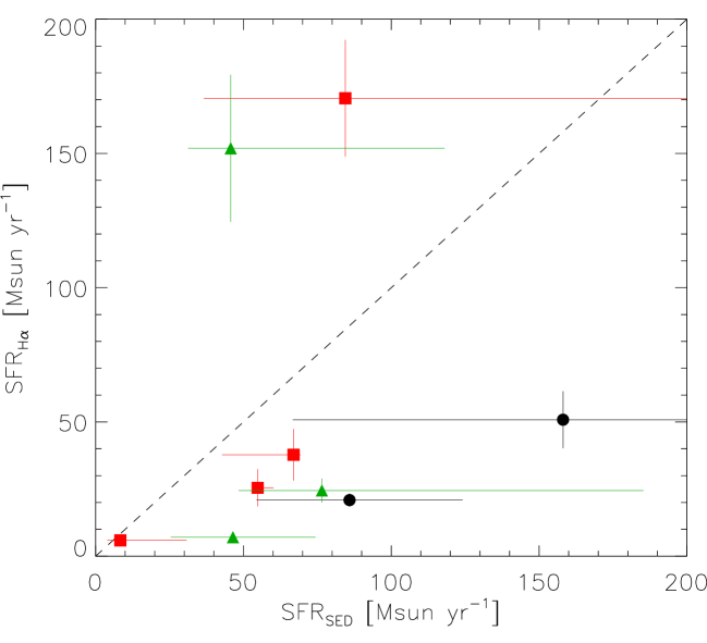
Figure 4: Comparison of H$\alpha$ SFR with [O ii] (left) and photometric (right) SFRs. The dashed line indicates $y=x$. Black dots, red squares, green triangles correspond respectively to objects classified (see section 4.1) as rotating disks (RD), perturbed rotators (PR) and merging systems (MS).

3.2 Morphologies

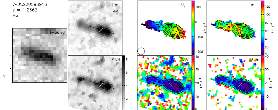
Figure 18: Similar as Figure 14 for VVDS220596913. The North feature is compatible with sky line residuals. $I$-band map is a CFH12K/CFHT image.

For each galaxy of our sample we have estimated the inclination from the $I$-band CFHT images using the GALFIT software (Peng et al., 2002). We have used CFHT legacy survey images with best seeing ($<$0.65″) for VVDS-02h field galaxies (Figures 14 to 17) and CFH12K/CFHT (McCracken et al., 2003) images for VVDS-22h field galaxies (Figures 18 to 22). GALFIT convolves a point spread function (PSF) with a model galaxy image based on the initial parameter estimates fitting a Sersic (1968) profile. Finally, GALFIT converges into a final set of parameters such as the Sersic index, the center, the position angle, and the axial ratio. Residual maps were used to optimize the results. Since the morphological inclination is used as input for kinematical modeling, we have imposed the morphological position angle of the major axis to be equal to the kinematical one (determined in section 3.3.2). When the morphological position angle is a free parameter, the agreement with the kinematical one is better than 25^∘ except for galaxies which have a morphology compatible with a galaxy seen face-on within the uncertainties, as it would be the case for local disks (Epinat et al., 2008a, b). This agreement is also true for some of the galaxies that we have classified as merging systems (see section 4.1 and individual comments in Appendix A). For mergers, the use of a fit relying on a disk hypothesis is undoubtly less meaningful than for relaxed systems. However, this fitting method enables to study the whole sample in an homogeneous way.

Epinat et al. (2009) have shown that observation of high redshift disk galaxies, strongly affected by beam smearing effects, have a disk inclination difficult to retrieve. The uncertainty on the inclination is the main source of errors in the rotational velocity determinations and thus on the Tully-Fisher relation, on the mass determination and on the mass assembly history. The extreme cases are provided by galaxies appearing face-on or edge-one from broad-band imagery: the radial velocity field of a face-on galaxy may show a velocity gradient indicating that the disk is not face-on; alternatively, an edge-on disk appears thicker and leads to an underestimation of the inclination. In order to check the disk inclinations determined by GALFIT, we have compared them to the ones computed using a simple correction provided in Epinat et al. (2009). They modeled inclined thin disks having exponential or flat truncated luminosity profiles with scale lengths from 2 to 6 kpc, observed at redshift $z=1.7$ with a seeing of 0.5″ and a sampling of 0.125″. They introduced a parameter $C$ in order to recover the true inclination $i$ from the seeing FWHM ($s$) and the measured major ($a_{m}$) and minor ($b_{m}$) axis lenghts (FWHMs) estimated in arcseconds from a 2D gaussian fitting :

$$\cos{i}=\frac{b}{a}=\sqrt{\frac{b_{m}^{2}-C^{2}\times s^{2}}{a_{m}^{2}-C^{2}\times s^{2}}}$$ (7)

where $a$ and $b$ are actual major and minor axis lengths (FWHMs) on the sky plane. The parameter $C$ represents the fraction of the seeing by which both measured minor and major axis are quadratically overestimated. In Epinat et al. (2009), it is shown that $C=1.014\pm 0.002$ for an exponential luminosity profile and $C=1.015\pm 0.010$ for a flat and truncated luminosity profile. This means that these smooth luminosity profiles can be satisfactorily described by a gaussian function. We have used $C=1.014$ to confirm the inclinations determined from the GALFIT fitting procedure. We have used the inclination determined from direct axis measurements for some objects for which GALFIT failed to converge into a realistic model. Except for those galaxies, GALFIT typically gives a disc component with a Sersic index of one and typical associated uncertainties ranging from 0.2 to 0.5.

In order to evaluate error bars on the inclination, the uncertainty on both major and minor axis lengths has been taken into account. Assuming that the error $\Delta$ is the same for both axes, we have computed upper and lower limits for the inclination reported in Table LABEL:table_kin following:

$$i_{max}=acos\left[\frac{b-\Delta}{a+\Delta}\right]$$ (8)

$$i_{min}=acos\left[\frac{b+\Delta}{a-\Delta}\right]$$ (9)

The typical uncertainty is $\Delta=0.25$″ (about one third the seeing).

3.3 Kinematics of the ionized gas

3.3.1 $H\alpha$ kinematics

Table 4: Kinematical parameters

VVDS ID	$z_{H\alpha}$	Inclination	Position Angle	$r_{t}$	$V_{t}$	Residuals ($V$)	$\chi^{2}$	$V_{t}/r_{t}$
		∘	∘	″	$km\leavevmode\nobreak\ s^{-1}$	$km\leavevmode\nobreak\ s^{-1}$		$km\leavevmode\nobreak\ s^{-1}$ kpc-1
(1)	(2)	(3)	(4)	(5)	(6)	(7)	(8)	(9)
020116027	1.53022	44 ${}^{+12}_{-23}$	219 $\pm$ 8	0.12	32	8	2.4	30
020182331	1.22832	52 ${}^{+9}_{-13}$	244 $\pm$ 6	0.55	134	18	1.2	29
020147106	1.51949	37 ${}^{+15}_{-37}$	307 $\pm$ 11	0.12	30	3	0.7	29
020261328	1.52891	47 ${}^{+12}_{-21}$	192 $\pm$ 5	0.77	195	12	2.2	30
220596913	1.26619	66 ${}^{+6}_{-7}$	253 $\pm$ 5	2.80	325	16	3.5	13
220584167	1.46588	49 ${}^{+9}_{-13}$	178 $\pm$ 1	1.24	280	15	6.6	26
220544103	1.39659	61 ${}^{+7}_{-10}$	205 $\pm$ 7	6.73	762	17	2.8	13
220015726	1.29300	25 ${}^{+21}_{-25}$	184 $\pm$ 1	0.12	323	16	6.8	309
220014252	1.31014	48 ${}^{+10}_{-15}$	137 $\pm$ 3	0.12	103	13	2.6	99

(1) Source VVDS identification number, (2) Geocentric SINFONI spectroscopic redshift deduced from model fitting, (3) Morphological inclination from CFHT $I$-band images, (4) Kinematical Position Angle of the major axis from North to East deduced from model fitting, (5) Characteristic radius of the kinematical model, (6) Characteristic velocity of the kinematical model, (7) Weighted standard deviation of the residual velocity map, (8) Reduced $\chi^{2}$ of the fit, (9) Inner velocity gradient derived from the model.

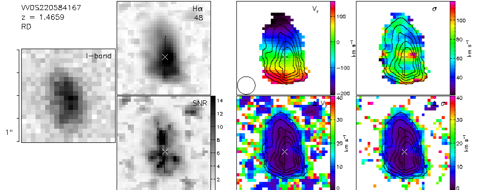
Figure 19: Similar as Figure 18 for VVDS220584167. The North-West feature is compatible with sky line residuals.

The SINFONI data were analysed using routines written under IDL environment . Our main goal was to determine the kinematics of the ionised gas using the strongest emission line, H$\alpha$. In order to increase the signal to noise ratio without degrading the spatial resolution, we have performed a sub-seeing spatial gaussian smoothing (FWHM$=$2 pixels) on the data cube (the mean seeing is around 0.65″ i.e. 5 pixels). For each galaxy of the sample we fit the spectrum around H$\alpha$ to a single gaussian function in order to characterize the emission line, and a pedestal to characterise the continuum. To minimize the effects of sky lines residuals on line parameters determination, the sky spectrum has been used in the fitting procedure in order to lower the weight of strong emitting sky lines wavelengths. From these fitting techniques it was possible, for each source, to recover the line flux map, the velocity field and the velocity dispersion map after correcting for instrumental dispersion (around 2.75Å) measured on sky lines. 2D error maps have also been derived for each quantity from the fitting procedure. These are statistical errors that take into account the error spectrum and that indicate the accuracy of the fit for each parameter. A signal-to-noise ratio map has been computed, the signal beeing the intensity of the fitted line and the noise beeing the standard deviation of the residual spectrum. These maps are presented in Figures 14 to 22. The velocity maps have been masked using several criteria: we have imposed (i) the line width to be larger than the one of the spectral PSF (the major part of the white pixels in the velocity dispersion error maps), (ii) the uncertainty on the velocity to be less than 30 $km\leavevmode\nobreak\ s^{-1}$ and (iii) the signal-to-noise ratio to be larger than $\sim 2$ ($1.5$ for the faintest object VVDS020182331). We also made a careful visual inspection in the spectrum to remove outer regions validating the criteria but for which the line was associated with strong sky residuals (see Figures 18 and 19).

3.3.2 Model fitting

Table 5: Mass parameters

VVDS ID	$V_{max}$	$R_{last}$	$r_{1/2}$	$\sigma_{0}$	$V_{max}/\sigma_{0}$	$M_{star}$	$M_{dyn}$	$M_{\theta}$	$M_{\sigma}$	$M_{\theta}/M_{\sigma}$	$M_{halo}$	Class
	$km\leavevmode\nobreak\ s^{-1}$	$kpc$	$kpc$	$km\leavevmode\nobreak\ s^{-1}$		$10^{10}\,{\rm M_{\odot}}$	$10^{10}\,{\rm M_{\odot}}$	$10^{10}\,{\rm M_{\odot}}$	$10^{10}\,{\rm M_{\odot}}$		$10^{10}\,{\rm M_{\odot}}$
(1)	(2)	(3)	(4)	(5)	(6)	(7)	(8)	(9)	(10)	(11)	(12)	(13)
020116027	32 ${}^{+29}_{-5}$	9.7	2.9	45 $\pm$ 13	0.7 ${}^{+1.2}_{-0.3}$	1.2 ${}^{+1.7}_{-0.5}$	5.5 ${}^{+4.1}_{-2.7}$	0.2 ${}^{+0.6}_{-0.1}$	5.3 ${}^{+3.5}_{-2.6}$	0.0 ${}^{+0.3}_{-0.0}$	0.5	MS
020182331	134 ${}^{+32}_{-14}$	6.3	4.5	71 $\pm$ 34	1.9 ${}^{+2.6}_{-0.8}$	5.8 ${}^{+1.0}_{-1.9}$	4.1 ${}^{+3.2}_{-1.7}$	2.6 ${}^{+1.4}_{-0.6}$	1.5 ${}^{+1.8}_{-1.1}$	1.8 ${}^{+8.4}_{-1.1}$	43.9	PR
020147106	30 ${}^{+\infty}_{-7}$	9.1	2.0	80 $\pm$ 8	0.4 ${}^{+\infty}_{-0.1}$	1.7 ${}^{+0.1}_{-0.6}$	27.6 ${}^{+\infty}_{-5.8}$	0.2 ${}^{+\infty}_{-0.1}$	27.4 ${}^{+6.4}_{-5.7}$	0.0 ${}^{+\infty}_{-0.0}$	0.4	PR
020261328	194 ${}^{+125}_{-31}$	6.4	1.2	55 $\pm$ 17	3.5 ${}^{+4.9}_{-1.3}$	0.6 ${}^{+1.8}_{-0.4}$	19.6 ${}^{+19.8}_{-9.0}$	5.6 ${}^{+9.7}_{-1.7}$	14.0 ${}^{+10.1}_{-7.4}$	0.4 ${}^{+1.9}_{-0.2}$	110.1	PR
220596913	177 ${}^{+13}_{-7}$	12.7	8.7∗	76 $\pm$ 20	2.3 ${}^{+1.1}_{-0.6}$	8.5 ${}^{+2.7}_{-4.1}$	13.0 ${}^{+3.7}_{-2.5}$	9.3 ${}^{+1.4}_{-0.7}$	3.7 ${}^{+2.3}_{-1.7}$	2.5 ${}^{+2.9}_{-1.1}$	98.7	MS
220584167	280 ${}^{+81}_{-31}$	10.9	7.9∗	47 $\pm$ 22	5.9 ${}^{+8.5}_{-2.3}$	12.1 ${}^{+10.9}_{-5.0}$	21.1 ${}^{+14.5}_{-5.0}$	20.0 ${}^{+13.2}_{-4.3}$	1.1 ${}^{+1.3}_{-0.8}$	18.1 ${}^{+90.7}_{-11.6}$	346.1	RD
220544103	146 ${}^{+19}_{-9}$	10.9	5.5	70 $\pm$ 17	2.1 ${}^{+1.1}_{-0.5}$	5.1 ${}^{+2.3}_{-3.1}$	10.3 ${}^{+4.2}_{-2.8}$	5.4 ${}^{+1.5}_{-0.7}$	4.9 ${}^{+2.7}_{-2.1}$	1.1 ${}^{+1.4}_{-0.5}$	51.0	MS
220015726	323 ${}^{+\infty}_{-135}$	6.4	2.7	38 $\pm$ 25	8.5 ${}^{+\infty}_{-5.5}$	6.2 ${}^{+5.7}_{-1.6}$	16.7 ${}^{+\infty}_{-11.3}$	15.5 ${}^{+\infty}_{-10.3}$	1.2 ${}^{+2.1}_{-1.0}$	13.2 ${}^{+\infty}_{-11.6}$	591.3	RD
220014252	103 ${}^{+39}_{-13}$	9.2	4.4	92 $\pm$ 19	1.1 ${}^{+0.8}_{-0.3}$	6.1 ${}^{+1.0}_{-3.6}$	10.2 ${}^{+5.7}_{-3.5}$	2.3 ${}^{+2.1}_{-0.6}$	7.9 ${}^{+3.7}_{-3.0}$	0.3 ${}^{+0.6}_{-0.1}$	19.4	PR

(1) Source VVDS identification number, (2) Maximum velocity deduced from model fitting, (3) Maximum radius of the kinematical maps, (4) Half light radius corrected for the beam smearing (an asterisk indicates that it has been computed from the $I$-band image), (5) “1/error”-weighted mean local velocity dispersion, (6) Ratio of the maximum rotation velocity (2) over the local velocity dispersion (5), (7) Stellar mass, (8) Total dynamical mass, (9) Rotation mass, (10) Dispersion mass, (11) Ratio of the dynamical masses, (12) Halo mass, (13) Kinematical classification (RD: Rotating Disk, PR: Perturbed Rotation, MS: Merging System).

To analyze the velocity fields of high redshift galaxies, four toy rotation curve models used in the literature (an exponential disk by Förster Schreiber et al., 2006; Cresci et al., 2009, an isothermal disk by Spano et al., 2008, an arctangent function by Puech et al., 2008 and a flat rotation curve by Wright et al., 2007, 2009 described hereafter) have been tested on a sub-sample of around 150 data cubes of nearby galaxies part of the GHASP sample which have been projected at high redshift (Epinat et al., 2009). These models consist of two parameters rotation curves that have various shapes, mainly the plateau (decreasing, increasing or flat) and the presence or not of an inner velocity bump. By comparing the parameters determined from high resolution and projected data, Epinat et al. (2009) have shown that the simple model used by Wright et al. (2007, 2009) leads to the best estimation of the kinematical parameters in average. The high resolution rotation curve (velocity $V$ as a function of the radius $r$) of this model is given by:

$$V(r)=V_{t}\frac{r}{r_{t}}$$ (10)

when $r\leq r_{t}$ and

$$V(r)=V_{t}$$ (11)

when $r>r_{t}$.

In the present work, this fit was attempted for all sources on their velocity field using the associated velocity error map in order to evalutate which ones are compatible with rotating disks. For objects that we have classified as merging systems (section 4.1), fitting rotating disks on substructures has been attempted and discussed in Appendix A. The high resolution model is convolved with the seeing measured on the PSF stars and by the 2-pixels gaussian smoothing applied on the data cubes. The parameters of the model are the position angle of the major axis (measured from North to East), the inclination, the center, the systemic velocity, the plateau of the rotation curve $V_{t}$ and the radius $r_{t}$ at which the plateau is reached.

This model fitting procedure described in details in Epinat et al. (2009) is based on a $\chi^{2}$ minimization. One main concern for fitting the data is that the actual high resolution line flux distribution is unknown. We have assumed that the observed line flux is representative of the high resolution one. Furthermore, due to projection effects, kinematical models are affected by a degeneracy between the rotation velocity $V(r)$ and the inclination. Even for local resolved galaxies, this degeneracy leads to large error bars on kinematical inclinations (Epinat et al., 2008a, b). Due to the low sampling, this degeneracy can not be ruled out for high redshift galaxies. We have fixed the inclination to the morphological value determined from $I$-band continuum images as described in section 3.2.

From the best fit model, we have computed a model velocity dispersion map. This model velocity dispersion map only includes the enlargement of the profiles due to the unresolved velocity gradient because of beam smearing effects (see Epinat et al., 2009 for analytical computation). It does not include enlargement due to the physics of the gas. Thus by subtracting quadratically the model to the measured velocity dispersion map, we are able to recover the local velocity dispersion noted hereafter $\sigma_{0}$. In order to take into account the uncertainty on the velocity dispersion map while computing the mean velocity dispersion, we have used a weight inversely proportional to the error. The same procedure has been applied while computing the mean velocity residual.

The results of this fitting procedure are presented in Table LABEL:table_kin. It contains the redshifts determined from SINFONI data, the morphological inclination used for the kinematical model, the kinematical position angle, the rotation curve parameters $r_{t}$ and $V_{t}$, the mean velocity residual, the reduced $\chi^{2}$ of the fit and the inner velocity gradient computed by the models. The center has been fixed to match the maximum of the flux distribution except for VVDS220584167 and VVDS220014252 (see Appendix A) since the determination of the kinematical center is severaly affected by the low spatial resolution as underlined in Epinat et al. (2009). Since no clear turnover is reached in the velocity fields and due to a symmetrization process, the center could be offset by more than 0.5″when let free, which is unrealistic. This biases the maximum velocity determination since the extent appears to be larger on the one side than on the other. The bias depends on the offset. It also changes the value of the geocentric spectroscopic redshift to the value corresponding to the center. However, the position angle of the major axis remains a stable parameter. The centers used are displayed in Figures 14 to 22. The maximum velocity suggested by the models is sytematically higher than the maximum velocity deduced from the maps computed as

$$V_{max,\leavevmode\nobreak\ map}=\frac{\textup{v}_{max}-\textup{v}_{min}}{2\times\sin{i}}$$ (12)

where $\textup{v}_{max}$ and $\textup{v}_{min}$ are the maximum and minimum values of the velocity field and $i$ is the inclination (see Table LABEL:table_tf). Indeed, the maximum velocity of a rotating disk is observed along the major axis. Due to beam smearing effects, the velocities measured along the major axis are lowered by the contribution of off-axis regions. The beam smearing may also affect the velocity gradients observed in merging systems velocity fields. For a given sampling, this effect is more pronounced for small galaxy.

3.3.3 Dynamical masses

To follow mass assembly accross the cosmic time, it is worth comparing dynamical masses and stellar masses even if uncertainties for both are rather large.

Given our high resolution 3D data on rotating disk candidates, the most robust mass estimate is the enclosed mass estimate. However a mass estimate requires several assumptions. First of all, the system has to be relaxed. The geometry of the system also has important consequences. If we consider that the mass is principally contained in spheroidal haloes, the enclosed mass $M_{\theta}$ at radius $R$ can be expressed as follow:

$$M_{\theta}=\frac{V^{2}R}{G}$$ (13)

$V$ beeing the velocity at radius $R$.

For some of the galaxies of our sample, there is no strong evidence for rotation and their kinematics are compatible with slowly rotating spherical systems, since the velocity gradient is lower than the velocity dispersion. For spherical, bound and dynamically relaxed systems with random motions, the virial mass is more appropriate than the enclosed mass:

$$M_{virial}=\frac{C\times\sigma^{2}\leavevmode\nobreak\ r_{1/2}}{G}$$ (14)

The parameter $C$ depends on the mass distribution and the geometry of the system, $r_{1/2}$ is the half light radius and $\sigma$ is the mean random velocity. Binney & Tremaine (2008) suggest that $C=2.25$ is an average value of known galactic mass distribution models.

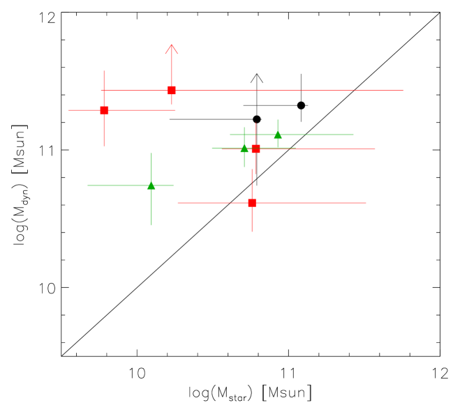
Figure 5: Comparison between total dynamical (y-axis) and stellar (x-axis) masses in log units. Black dots, red squares, green triangles correspond respectively to objects classified (see section 4.1) as rotating disks (RD), perturbed rotators (PR) and merging systems (MS). The solid line represents $y=x$.

Figure 6: Comparison between rotation (y-axis) and dispersion (x-axis) masses in log units. Black dots, red squares, green triangles correspond respectively to objects classified (see section 4.1) as rotating disks (RD), perturbed rotators (PR) and merging systems (MS). The solid line represents $y=x$.

Since our objects clearly show both rotation and dispersion motions, one might take into account both components to compute the total dynamical mass. To do that, we have to apply an “asymmetric drift correction” term (Meurer et al., 1996) which involves radial gradients of the gas surface density, the gaseous velocity dispersion, and the disk scale height. To simplifiy, we assume that the disk scale height radial gradient is null as well as the dispersion one since we do not see clear radial dependency in our data. Thus, assuming that the gas is in dynamical equilibrium and that the gas velocity ellipsoid is isotropic, the total dynamical mass can be expressed as:

$$M_{dyn}=M_{\theta}+M_{\sigma}=\frac{V^{2}\leavevmode\nobreak\ R}{G}+\frac{\sigma^{2}\leavevmode\nobreak\ R^{3}}{G\leavevmode\nobreak\ h^{2}}$$ (15)

where $h$ is the gas surface density disk scale length when described by a gaussian function and $\sigma$ is the local velocity dispersion at radius $R$. We note the two terms of equation 15 respectively $M_{\theta}$ and $M_{\sigma}$ since they respectively refer to rotation and dispersion masses.

The first term $M_{\theta}$ is equal to the enclosed mass within radius $R$. The second term $M_{\sigma}$ is similar to the virial mass. Indeed, the gas surface density is well described by a gaussian function with $r_{1/2}=h\sqrt{2\ln{2}}$. The virial mass is thus equal to the asymmetric drift correction term at

$$R=(C/2\ln{2})^{1/3}\leavevmode\nobreak\ r_{1/2}\sim 1.2\leavevmode\nobreak\ r_{1/2}$$ (16)

In Table LABEL:table_mass, we have computed $M_{dyn}$, $M_{\theta}$ and $M_{\sigma}$ at $R_{last}$, radius of the last point for which a velocity measurement is done. Since the actual rotation velocity amplitude mainly depends on the true inclination of the system, we have used the uncertainties on the inclination to compute upper and lower limits for the rotation mass computed from equation 13. We have also used the maximum velocity $V_{max}$ derived from our kinematical modeling within the radius $R_{last}$ ($V_{t}$ when $R_{last}>r_{t}$). Since we assumed the velocity dispersion to be constant, we used the “1/error”-weighted mean local velocity dispersion corrected for beam smearing effects $\sigma_{0}$ to compute the dispersion mass. The half light radius $r_{1/2}$ has been determined for each galaxy from a two dimension gaussian fitting on line flux maps provided in Figures 14 to 22. The half light radius measured on $I$-band CFHT images is in average about $1.1$ the H$\alpha$ one. For two galaxies (VVDS220584167 and VVDS220596913), since the fit on the H$\alpha$ line flux maps did not converge, we thus used the half light radius measured on CFHT $I$-band images divided by $1.1$. For each galaxy, $r_{1/2}$ has been corrected for the beam smearing using a quadratical subtraction of half the seeing disk. All these parameters are stored in Table LABEL:table_mass together with the dynamical classification defined in section 4.1 and two indicators of dynamical support ($V_{max}/\sigma_{0}$ and $M_{\theta}/M_{\sigma}$) on which the classification partly relies. $R_{last}$ and $r_{1/2}$ beeing approximatively linearly correlated, these two dynamical support indicators are directly linked since:

$$\frac{M_{\theta}}{M_{\sigma}}=2\ln{2}\left(\frac{R_{last}}{r_{1/2}}\right)^{2}\left(\frac{V_{max}}{\sigma_{0}}\right)^{2}$$ (17)

The use of the mass estimates instead of $V_{max}/\sigma_{0}$ ratio enables to know which is the main contribution.

For galaxies classified as mergers (see section 4.1), this method to compute the mass is more approximative than for rotating disks. Indeed, the rotation velocity and the extent measurements used to compute the rotation mass component $M_{\theta}$ as well as the half light radius measurement used to compute the dispersion mass component $M_{\sigma}$ are derived using disk hypothesis. However, since it is difficult to extract unambiguously the components, this method gives a trend (see Appendix A for individual details).

As shown in Figure 5, the total dynamical mass is higher or equal than the stellar mass within the uncertainties. The difference between dynamical and stellar masses could be even larger if for some galaxies the turnover in the rotation curve is not reached or if the extent of the stellar distribution is much larger than the gas one. This trend shows that in most of the cases, the gravitational potential is mainly due to gas and dark matter.

Rotating disks (dynamical classes are defined in section 4.1) have both large dynamical and stellar masses (around $10^{11}\,{\rm M_{\odot}}$) while mergers and perturbed rotators present a larger mass range. The comparison between dynamical and stellar masses is discussed for each galaxy in Appendix A.

In Figure 6 comparing rotation and dispersion masses, rotation-dominated systems are clearly distinguished from dispersion-dominated ones. Indeed, on the one hand, for the two galaxies classified as rotating disks (VVDS220584167 and VVDS220015726), the rotation mass is higher than the dispersion mass by a factor larger than 13 showing that their gravitational support is rotation dominated. On the other hand, VVDS020116027 and VVDS020147106 are clearly dominated by random motions ($M_{\sigma}/M_{\theta}>10$) even if inclination effects may lead to slightly higher values. The five remaining galaxies with $M_{\theta}/M_{\sigma}\sim 1$ show both rotation and dispersion gravitational supports.

3.3.4 Halo masses

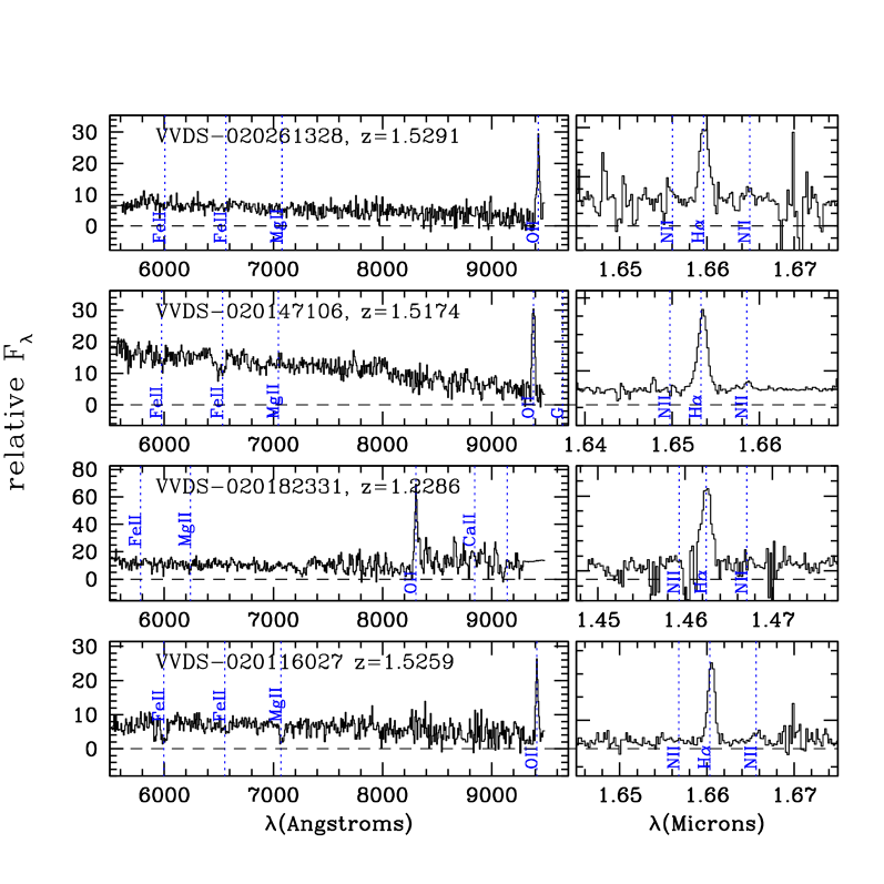
Figure 7: VIMOS optical spectra from which the original redshifts were derived (left) and SINFONI (right) 1D spectra around the H$\alpha$ line for the four VVDS-02h field galaxies. SINFONI spectra have been produced summing spectra of all spatial resolution elements with detected H$\alpha$ emission. The main emission and absorption lines are marked and labeled for each sources. The line wavelengths are computed using the redshifts deduced from SINFONI data (Table LABEL:table_kin).

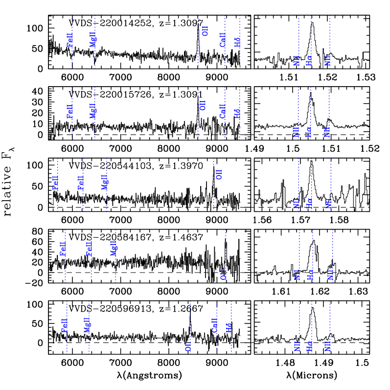
Figure 8: Similar as Figure 7 for the five VVDS-22h field galaxies.

We have estimated the total halo mass ($M_{halo}$) using a spherical virialized collapse model (Peebles, 1980; White & Frenk, 1991; Mo & White, 2002). We assumed that the plateau has been reached in our observations and that the plateau velocity $V_{max}$ traces the modeled halo circular velocity.

$$M_{halo}=0.1\leavevmode\nobreak\ H_{0}^{-1}\leavevmode\nobreak\ G^{-1}\leavevmode\nobreak\ \Omega_{m}^{-0.5}\leavevmode\nobreak\ (1+z)^{-1.5}\leavevmode\nobreak\ V_{max}^{3}$$ (18)

where $H_{0}$ is the local Hubble constant, $\Omega_{m}$ is the local matter density, $G$ is the universal gravitational constant and $z$ is the redshift of the galaxy.

In the cases where our models indicate that the plateau is not reached within the observation, we have used the maximum velocity derived from our kinematical modeling within the radius $R_{last}$ instead of the plateau velocity of the model $V_{t}$ since the plateau is not constrained correctly. The values are available in Table LABEL:table_mass.

If we assume that the length of the halo is the size that a galaxy should have in order that its enclosed mass is equal to the halo mass, then for our sample, the halo length is $113\pm 73$. It is larger for fast rotating disks since:

$$R_{halo}=0.1\leavevmode\nobreak\ H_{0}^{-1}\leavevmode\nobreak\ \Omega_{m}^{-0.5}\leavevmode\nobreak\ (1+z)^{-1.5}\leavevmode\nobreak\ V_{max}$$ (19)

These total halo masses have no physical meaning for galaxies which are not gravitationally supported by rotation. For galaxies having a ratio $V_{max}/\sigma_{0}$ larger than unity, the total halo masses range from 0.2 to 6.0$\times 10^{12}\,{\rm M_{\odot}}$. These values are much larger than the measured dynamical masses. At redshift $z=1.5$, a galaxy with the same maximum rotation velocity than a $z=0$ galaxy is supposed to have a total halo mass lower by a factor $\sim 4$. Our rotation dominated sources have $M_{\theta}/M_{halo}\sim 0.049\pm 0.015$ in average. This value cannot be directly compared to the fraction of baryonic matter to total matter $\Omega_{b}/\Omega_{m}=0.171$ (Komatsu et al., 2009) because $M_{\theta}$ may contain a noticeable fraction of dark matter. Indeed, for comparison, typical halo masses measured from mass model derived from rotation curves at the last HI radius for nearby galaxies larger than 18 kpc is around $25\times 10^{10}\,{\rm M_{\odot}}$ (Blais-Ouellette et al., 2001; Spano et al., 2008). Taking into account that the values computed for local galaxies are measured, in average, at a radius twice as large as the sample of high redshift galaxies, the total cosmological halo mass for high redshift galaxies are still much larger than the total halo mass measured for local galaxies from rotation curves.

3.4 Search for type 2 AGN and metallicity

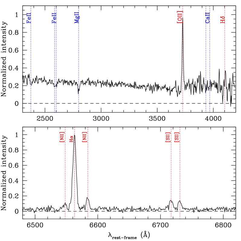
Figure 9: Combined spectrum of the nine VVDS galaxies at $1.2<z<1.6$ observed with VIMOS (top) and SINFONI (bottom), in arbitrary flux units and rest frame wavelengths. The position of the main emission and absorption lines are indicated in red and blue respectively.

Along with the VIMOS optical spectra, we show in Figures 7 and 8 the integrated 1D SINFONI spectra around the H$\alpha$ line, resulting from the sum of all spatial resolution elements in the datacubes at the position of the sources. VIMOS and SINFONI combined spectra of the nine observed galaxies are shown in Figure 9. These are median spectra that have been computed using respectively [O ii] flux and H$\alpha$ flux to normalize each individual spectrum. One can clearly identify [N ii] $\lambda$6548 and [N ii] $\lambda$6584 emission lines, as well as the [S ii] doublet at 6717 and 6731Å in the SINFONI combined spectrum. The low [N ii] $\lambda$6584/H$\alpha$ and [S ii] $\lambda\lambda$6717,6731/H$\alpha$ ratios ($=0.13$ and $0.23$ respectively) indicate the lack of AGN contribution in our sample. We further performed a careful inspection of the spatial distribution of the [N ii] $\lambda$6584/H$\alpha$ ratio for each galaxy. [N ii] $\lambda$6584 line flux maps were derived similarly to H$\alpha$ ones (see section 3.3.1). However, since the [N ii] $\lambda$6584 flux is rather weak, we used the H$\alpha$ line to constrain the line position. We do not find any significant peak in the flux ratio maps, contrary to Wright et al. (2009) who found an AGN in two of their six $z\sim 1.6$ galaxies. This lack of AGN contribution is further supported by other indicators.

• the quite low mean value of reddening ($E(B-V)\sim 0.3$ or $A_{V}\sim 1$) measured in our sample galaxies is against any dusty AGN alternative

• we do not detect any strong [Ne iii] $\lambda$3869 or [Ne v] $\lambda$3426 emission in the VIMOS composite spectrum which would be a clear signature of Sey2-like activity (e.g. Zakamska et al., 2003)

• no evidence for Sey2-like activity is found in X-ray data. Indeed, we have checked in the HEASARC archive that no X-ray counterpart was yet detected at less than 30″ from our objects. Moreover, when existing, the counterparts are closer to brighter objects.

Note also that type 1 AGN are excluded from the parent VVDS sample on the basis of the presence of broad emission lines in the VIMOS spectrum.

The [N ii] $\lambda$6584/H$\alpha$ ratio can be used to estimate roughly the typical metallicity of our sample. Using the last calibrations proposed by Pérez-Montero & Contini (2009), we have estimated a rather low oxygen abundance $12+log(O/H)=8.37$, corresponding to half the solar metallicity (see Queyrel et al., 2009 for a full discussion on the mass-metallicity relation).

4 Results

4.1 Kinematical classification

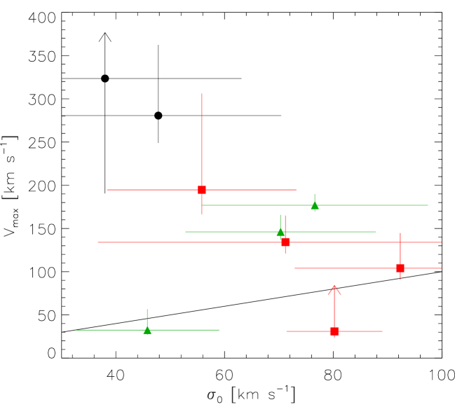
Figure 10: Maximum rotation velocity $V_{max}$ deduced from rotating disk model fitting as a function of “1/error”-weighted mean local velocity dispersion corrected for beam smearing effects $\sigma_{0}$. Black dots, red squares, green triangles correspond respectively to objects classified as rotating disks (RD), perturbed rotators (PR) and merging systems (MS). The solid line represents $y=x$.

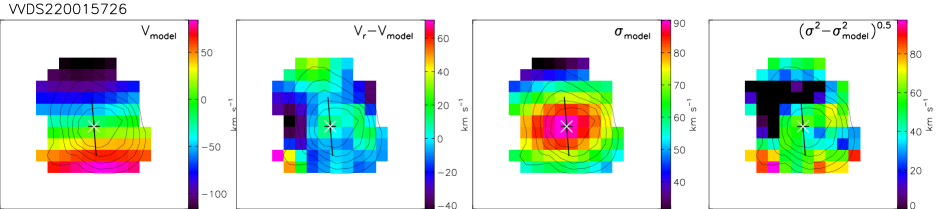
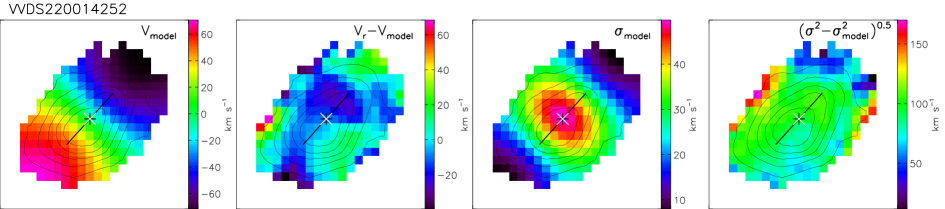
Figure 11: From left to right: Model velocity field, velocity field residuals, model velocity dispersion map and velocity dispersion map quadratic residuals. North is up, East is left. The center of the models is marked on each kinematical map with a black and white double cross. The solid line represents the orientation of the kinematical major axis and ends at half light radius measured on I-band images. The flux contours are overplotted.

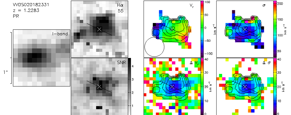
Figure 15: Similar as Figure 14 for VVDS020182331. The signal-to-noise threshold for this galaxy has been set to 1.5.

It has already been observed by other authors studying $z>1$ star-forming galaxies with 3D-spectroscopy (Law et al., 2007; Wright et al., 2007, 2009; Genzel et al., 2006, 2008; Förster Schreiber et al., 2006; Cresci et al., 2009) that the gaseous velocity dispersion of these objects is larger than at lower redshifts (Yang et al., 2008). As shown from kinematical modeling, an unresolved velocity gradient cannot account for high velocity dispersion values (Epinat et al., 2009). The kinematical classification as performed by Flores et al. (2006) on FLAMES/GIRAFFE data relies mainly on the ability to observe a signature of unresolved velocity gradient in the velocity dispersion map: rotating disks are defined as systems showing a regular velocity gradient and a central peak in the velocity dispersion map, where the actual velocity gradient is the steepest; systems with an offset velocity dispersion peak from the center, or without peak, are defined as perturbed rotators; the galaxies with no regular velocity gradient and no velocity dispersion central peak are classified as galaxies having complex kinematics. For systems with a high local velocity dispersion of the ionized gas, the velocity dispersion argument is thus not valid anymore. In Figure 11, we show examples of rotating disk models for two objects from our sample illustrating this point. For VVDS220015726 (first line) and VVDS220014252 (second line), the model velocity fields (first column) show that the kinematics of these objects reasonably match rotating disks (the second column shows the residual velocity fields). For VVDS220015726, the signature in the velocity dispersion map (third column) correctly matches the unresolved velocity gradient signature since the velocity dispersion map central signature (see Figure 15) is well removed when subtracting quadratically the model (last column of Figure 11). For VVDS220014252 which has a higher velocity dispersion, the model velocity dispersion map absolutely does not account for the observed velocity dispersion as demonstrated by the resemblance between corrected (last column of Figure 11) and uncorrected (see Figure 15) velocity dispersion maps.

The $\sim$0.65″ seeing continuum images from CFHT do not allow a morphological classification as accurate as performed by Neichel et al. (2008) from HST data on IMAGES sample. However, relying on line flux morphology, the kinematical maps derived from our SINFONI data and from attempts to fit a rotating disk model, we are able to derive a first order kinematical classification.

We defined rotating disks (RDs) as systems for which the rotation mass is higher than the dispersion mass (rotation dominated systems, see the two parameters $V_{max}/\sigma_{0}$ and $M_{\theta}/M_{\sigma}$ linked by equation 17 and given in Table LABEL:table_mass) as shown in Figure 6 and for which both velocity field and velocity dispersion map are described by rotating disk models. Mergers systems (MSs) are defined as systems with two spatially resolved components in the H$\alpha$ map and for which the velocity field is not described accurately by rotating disk models. Other systems are classified as perturbed rotators (PRs). They mainly show high velocity dispersions, higher than around 60 $km\leavevmode\nobreak\ s^{-1}$, and their velocity fields show some peculiarities not described by rotating disks.

Figure 10 shows a correlation between the maximum rotation velocity $V_{max}$ and the “1/error”-weighted mean local velocity dispersion corrected for beam smearing effects $\sigma_{0}$, in particular for rotating disks and perturbed rotators. The most massive galaxies (see Table LABEL:table_mass) are our two RDs. This would imply that the most massive disks are stable earlier or that stable disks can already be formed at these redshifts. Random motions convert in organized motions (rotation) more rapidly for massive systems.

From our classification, we obtain three clear major merging systems, two clear rotating disks and four perturbed rotators that could be either perturbed by minor merging events or by continuous gas accretion. The classification is summarized in column (10) of Table LABEL:table_mass and individual detailed comments on the kinematics and dynamics of each galaxy are provided in Appendix A.

4.2 The Tully-Fisher relation

Table 6: Magnitudes and maximum velocities

VVDS ID	KAB	BAB	$V_{max,\leavevmode\nobreak\ model}$	$V_{max,\leavevmode\nobreak\ map}$
	mag	mag	$km\leavevmode\nobreak\ s^{-1}$	$km\leavevmode\nobreak\ s^{-1}$
(1)	(2)	(3)	(4)	(5)
020116027	-22.7 $\pm$ 0.4	-21.8 $\pm$ 0.2	32 ${}^{+29}_{-5}$	23 ${}^{+21}_{-4}$
020182331	-22.3 $\pm$ 0.2	-21.7 $\pm$ 0.1	134 ${}^{+32}_{-14}$	114 ${}^{+27}_{-12}$
020147106	-22.8 $\pm$ 0.1	-22.1 $\pm$ 0.1	30 ${}^{+\infty}_{-7}$	21 ${}^{+\infty}_{-5}$
020261328	-21.6 $\pm$ 1.0	-21.1 $\pm$ 0.3	194 ${}^{+125}_{-31}$	82 ${}^{+53}_{-13}$
220596913	-23.2 $\pm$ 0.5	-22.6 $\pm$ 0.1	177 ${}^{+13}_{-7}$	153 ${}^{+11}_{-6}$
220584167	-24.2 $\pm$ 0.5	-23.1 $\pm$ 0.1	280 ${}^{+81}_{-31}$	198 ${}^{+57}_{-22}$
220544103	-23.2 $\pm$ 0.5	-22.5 $\pm$ 0.2	146 ${}^{+19}_{-9}$	108 ${}^{+14}_{-6}$
220015726	-23.2 $\pm$ 0.5	-22.1 $\pm$ 0.1	323 ${}^{+\infty}_{-135}$	189 ${}^{+\infty}_{-79}$
220014252	-23.3 $\pm$ 0.5	-22.6 $\pm$ 0.2	103 ${}^{+39}_{-13}$	84 ${}^{+32}_{-11}$

(1) Source VVDS identification number, (2) AB absolute magnitude in rest frame $K$-band, (3) AB absolute magnitude in rest frame $B$-band, (4) Maximum velocity derived from the model, (5) Maximum velocity derived from the maps (equation 12).

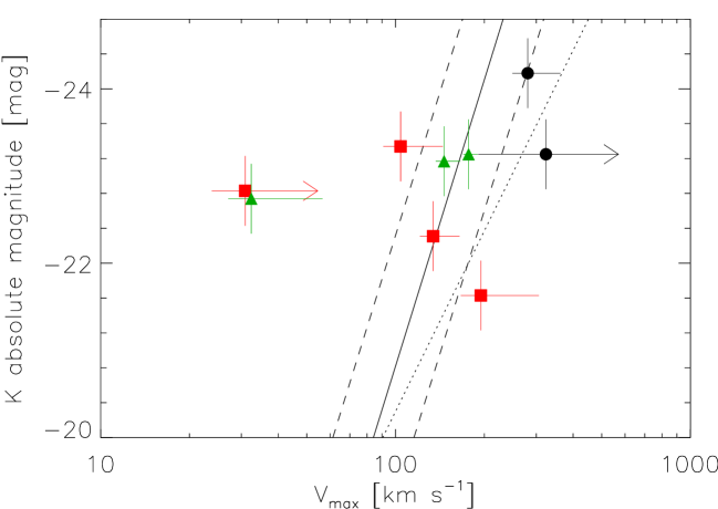
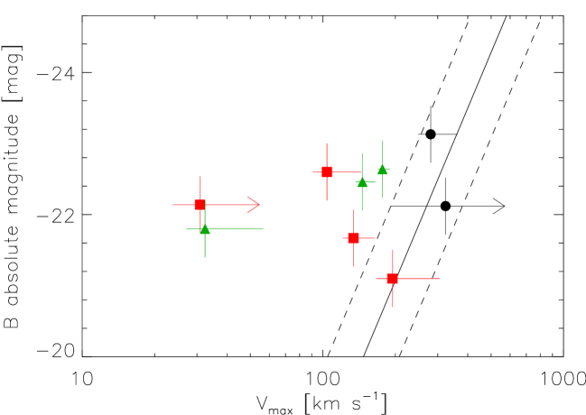
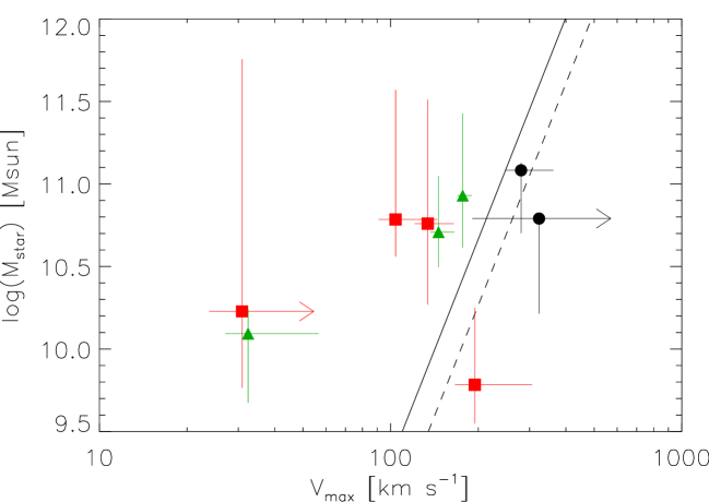
Figure 12: $K$-band (top), $B$-band (middle) and stellar mass (bottom) TFRs for our nine $z\sim 1.4$ galaxies. Black dots, red squares, green triangles correspond respectively to objects classified (see section 4.1) as rotating disks (RD), perturbed rotators (PR) and merging systems (MS). The maximum velocity has been determined from the rotating disk fit modeling. Top: the dotted line represents the local reference $K$-band TFR used by Puech et al. (2008) derived from H$\alpha$ on a SDSS sub-sample. Top and middle: the solid line represents respectively the local $K$-band and $B$-band TFRs derived from a local HI sample by Meyer et al. (2008) whereas the dashed lines represent the dispersion of the HI galaxies around these local relations. Bottom: the solid line represents the $z=0$ TFR derived by Bell & de Jong (2001). The dashed lines represent the $z=2.2$ TFR derived from SINS data by Cresci et al. (2009).

The Tully-Fisher relation (hereafter TFR) (Tully & Fisher, 1977) links the maximum rotation velocity to the actual flux or mass of a galaxy (via their logarithm). Extensive work has been produced in order to probe the evolution of the TFR with cosmic time in both $B$-band and $K$-band up to redshifts $z\sim 1.4$ (e.g. Fernández Lorenzo et al., 2009 for references). Since it requires a large sample of galaxies (more than $\sim$50 galaxies), high redshift TFR were derived from long-slit spectroscopy samples, except the ones derived by (i) Flores et al. (2006) and Puech et al. (2008) from FLAMES/GIRAFFE IFUs data at $z\sim 0.6$; (ii) Cresci et al. (2009) from SINFONI data at $z\sim 2.2$ and (iii) Swinbank et al. (2006) from lensed galaxies at $z\sim 1$ observed with GMOS.

In the frame of the present work, due to the small number of objects, we only look at the distribution of the different kinematical types accross the local TFR. We present the local TFR derived from HI data by Meyer et al. (2008) (solid line) since they provide both $K$-band (Figure 12, top) and $B$-band (Figure 12, middle) relations. Puech et al. (2008) used a subsample of SDSS sample (Pizagno et al., 2007) to derive a local reference TFR. The latter has been derived using $V_{80}$ velocities instead of maximum velocities (from H$\alpha$ kinematics) since they argue that their maximum velocity is statistically not measured (see Puech et al., 2008 and Pizagno et al., 2007 for details). We thus also plot this $K$-band reference TFR in Figure 12, top (dotted line).

For local samples with H$\alpha$ kinematical data, usually one has to exclude galaxies with low inclination because the uncertainty on their maximum velocity is high, but also galaxies with high inclination because of dust extinction in the disk that can bias the maximum velocity determination. For high redshift, as mentioned in section 3.2, the inclination is poorly known, thus we expect to observe both face-on and edge-on systems that we are not able to identify.

Absolute magnitudes in the desired rest-frame band (using the appropriate filter response curve) and stellar masses with their associated error bars for our objects were obtained from the same spectral energy distribution modeling than described in section 3.1 using the GOSSIP software (Franzetti et al., 2008). Stellar masses and the associated errors are provided in Table LABEL:table_mass whereas rest-frame $B$- and $K$-band absolute magnitudes and their associated errors determined from the PDF are provided in Table LABEL:table_tf. Uncertainties on $K$-band magnitudes are larger than for $B$-band. They result from the lack of any measurement of $K$ rest-frame ($\sim 3.5\mu$m) to constrain efficiently the SED fitting.

In Figures 12 top and middle, we respectively show the $K$- and $B$-band TFR for our nine $z\sim 1.4$ objects. The maximum velocities $V_{max}$ have been derived from the rotating disk models. $V_{max}$ is systematically higher when coming from the models that take into account the beam smearing effects (see Table LABEL:table_tf). On these Figures, to distinguish the three kinematical types we affected different colors and symbols (see caption). We see that the RD galaxies follow accurately the local $B$-band TFR as well as the PR with the highest $V_{max}$. These galaxies show a better agreement with the SDSS $K$-band TFR rather than the HI one. The two objects with no consequent rotation observed are the furthest from the local TFR (both $K$- and $B$-band). For the one classified as PR, this can be accounted for by the inclination. As for local galaxies, these galaxies have to be excluded from the TFR analysis because of the uncertainty on the inclination. The other objects classified as PR or MS stand on a restricted area on the TFR and present some correlation (if we exclude the slowest rotator) parallel to the local TFR, both in $B$- and $K$-bands. The three kinematical types seem to behave as the three kinematical types of Puech et al. (2008).

Given the strong evolution in luminosity with redshift and the fact that the $B$-band rest-frame magnitude is sensitive to short bursts of star formation, we also consider in Figure 12 (bottom) the stellar mass TFR which has the advantage of probing more closely the actual stellar mass build-up of galaxies. As for the absolute magnitude TFR, the two rotating disks follow the stellar mass TFR traced by Cresci et al. (2009) between $z\sim 1.5$ and $z\sim 2.5$.

A larger sample will be needed in order to provide more advanced conclusions on TFR evolution.

5 Discussion and conclusions

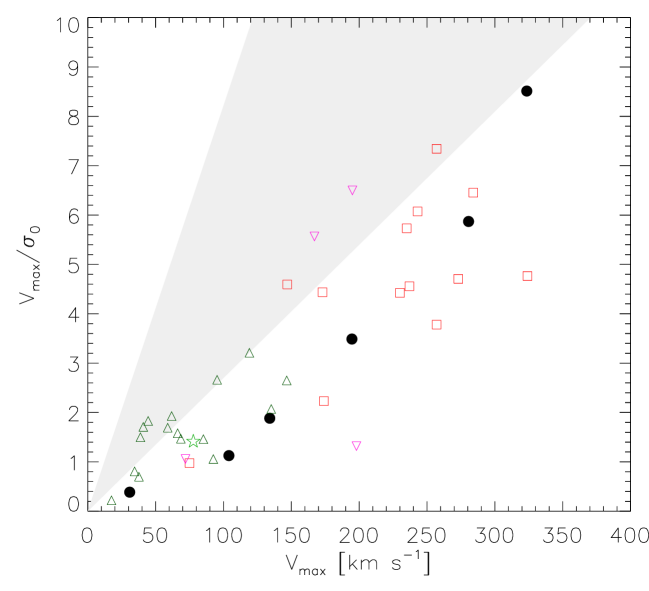
Figure 13: Ratio of the maximum rotation velocity $V_{max}$ (from modeling) with the mean local velocity dispersion corrected for beam smearing effects $\sigma_{0}$ as a function of the maximum rotation velocity. Black dots are our rotating disks (RD) and perturbed rotators (PR). The grey cone corresponds to the area covered by local rotating disk galaxies (GHASP sample, Epinat et al., 2009). Galaxies from the literature are also plotted: dark green triangles are from Law et al. (2007, 2009), light green star is from Stark et al. (2008), pink up side down triangles are rotating disks from Wright et al. (2007, 2009) and red squares are rotating disks from the SINS sample Genzel et al. (2008); Cresci et al. (2009). The maximum rotation velocities and the mean local velocity dispersion for the galaxies from Law et al. (2007, 2009) have been corrected for beam smearing using the recipes presented in Epinat et al. (2009), and a mean statistic inclination of 45^∘ has been used to deproject the velocities in the galaxy plane.

Using high spatial resolution near infrared integral field spectroscopy, we have produced a detailed analysis of the kinematical maps of nine galaxies with $1.2\leq z\leq 1.6$ selected from the VVDS. We have identified three major mergers systems, two massive rotating disks with total dynamical mass $>10^{11}\leavevmode\nobreak\ \,{\rm M_{\odot}}$, and four galaxies with an indication of rotation but with perturbed velocity maps, two of them with high gaseous velocity dispersion unseen in local isolated disks (Epinat et al., 2009). Our sample, although still small but comparable in size to other samples in the literature, has the advantage to be selected from an unbiased sample drawn from the $I$-band magnitude selected VVDS and with [OII]3727 $EW>50$Å.

The effects of beam smearing on the data (mean seeing around 0.65″ corresponding to around 5 kpc at these redshifts) have been taken into account in the interpretation of the kinematical maps in particular to correct the velocity dispersion maps from unresolved velocity gradients, using model fitting methods as done by Förster Schreiber et al. (2006) or Wright et al. (2007).

Finding three major merging systems, representing 30% of our sample, is a high occurence. We can compare this pair fraction to the measurements at lower redshifts: de Ravel et al. (2009) find that at $z\sim 1$ about 10% of galaxies with a stellar mass $M_{*}>10^{10}\leavevmode\nobreak\ \,{\rm M_{\odot}}$ are in pairs likely to lead to a major merger, making the merger rate in our higher redshift sample significantly higher. When taking into account typical merger timescales of $\sim 0.5-1$ Gyr, the high rate in our sample means that over a $\sim 3$ Gyr period virtually all galaxies with stellar mass $>10^{10}\leavevmode\nobreak\ \,{\rm M_{\odot}}$ will have undergone at least one major merger event. Although the observed sample is small, this result is comparable to the fraction of mergers in other samples at similar (Wright et al., 2009) or higher redshifts (Shapiro et al., 2008). In two of our merger systems, we can identify that one of the galaxies is compatible with a rotating disk, indicating that disk galaxies are indeed involved in merging events at these high redshifts.

The two massive rotating disks, with velocity dispersion maps indicating stable disks, confirm that massive rotating disks with total dynamical mass $M>10^{11}\leavevmode\nobreak\ \,{\rm M_{\odot}}$ are already well assembled at $z\sim 1.5$. The stability is underlined by the agreement of these galaxies with local Tully-Fisher relations obtained from local samples. These disks obviously need to have been assembled at earlier cosmic times, therefore requiring an early process of formation. These objects are comparable to some of the massive disks observed at similar redshifts by Wright et al. (2009), or at higher redshifts by Förster Schreiber et al. (2006), Genzel et al. (2008) and Law et al. (2009). However, we note that these disks are only about 20% of our sample.

Perturbed rotators are the dominant population in our sample with four galaxies over nine. These objects show perturbed velocity maps, two of them with high velocity dispersion, with a $V/\sigma_{0}$ lower than for typical rotating disks (Figure 13), indicating that the gravitational support is not mainly due to rotation. These objects are clearly a separate class not observed at lower redshifts. Their dynamical state is comparable to some of the galaxies observed by Förster Schreiber et al. (2006), Wright et al. (2009), or Law et al. (2009). At a resolution of a few kiloparsecs, we argue that it is difficult to disentangle whether the high velocity dispersion is produced by instabilities resulting from gas accretion e.g. along the filaments of the cosmic web, representing early-stage disks with a high cold gas fraction which fragmented under self-gravity and collapsed to form a starburst (Immeli et al., 2004b), or by gas rich minor merger events (e.g. Semelin & Combes, 2002). Indeed, both scenarios of continuous accretion of cold gas coming from cosmological filaments and frequent mergers of minor cold gas satellites may fuel the disk in fresh gas. If minor mergers (ranging from 10:1 to 50:1) are relatively significant, the relaxation processes will expulse the pre-existing stars from the disk to a spheroid structure or to a very thick disk not directly observable for high redshift galaxies. On the other hand, the formation of these structures would not perturb dramatically the kinematics of the disk, and thus would not be easily observable. Indirect signatures of the existence of a spheroid could be the stabilization of the gaseous disk, reducing the star formation out of merger phases and thus reducing the amount of sub-structures like H$\alpha$ or UV clumps in the disk. On the contrary, a very smooth accretion of diffuse gas coming from an extended halo or from the cosmological filaments will not be so efficient to form a stellar spheroid. Thus instabilities would be more numerous in the disks and possibly observable through deep imaging addressing the formation of clumps. For very minors mergers (e.g. mass ratio $>$ 100:1), the dwarf galaxies will be dislocated by the tidal field once they experience the gravitational field of the main galaxy. Thus, torn by tidal field, the accretion of very small companions will resemble very much to diffuse gas accretion. For a baryonic mass galaxy of $10^{10}\leavevmode\nobreak\ \,{\rm M_{\odot}}$, these satellites correspond to mass lower than $10^{8}\leavevmode\nobreak\ \,{\rm M_{\odot}}$. If they exist, due to the lack of spatial resolution, these galaxies are not observed, neither in observations nor in numerical simulations.

For two of the perturbed rotators observed in our sample (VVDS020147106 and VVDS220014252), the velocity maps are asymmetric and consistent with a small companion in the process of merging. More generally, these perturbed rotators indicate that disk build-up is fully on-going at the peak of cosmic star formation history.

Star formation rates in our sample are high, with an average of $\sim 55$ M_⊙ yr^-1, meaning that over the $\sim$1 Gyr between $z=1.6$ and $1.2$ more than $5\times 10^{10}\leavevmode\nobreak\ \,{\rm M_{\odot}}$ would be formed if this rate is sustained, comparable to the average dynamical mass. This seems to indicate that any external accretion should last only a limited time.

We have not found any evidence for type 2 AGN in our sample, (type 1 were already excluded from our parent galaxy sample). The average [N ii]/H$\alpha$ and [S ii]/H$\alpha$ ratios are typical of star-forming galaxies (Stasińska et al., 2006), and the [N ii]/H$\alpha$ 2D maps do not show a central excess of [N ii] which could indicate an AGN. Although we cannot exclude low luminosity or highly obscured AGN, this seems to indicate that the AGN and star formation phenomena may be only weakly connected in the main star-forming galaxy population.

The question of the assembly of galaxies via major dissipative mergers or internal secular processes has been recently highly debated in the literature. Genzel et al. (2008) advocated a secular process of assembly to form bulges and disks in massive galaxies at $z\sim 2$. Law et al. (2009) concluded that the high velocity dispersions they observe in most galaxies at $z\sim 2$ may be neither a ‘merger’ nor a ‘disk’, but rather the result of instabilities related to cold gas accretion becoming dynamically dominant. Our data seem rather to indicate that several processes are acting at these epochs. Among them, merging seems to play a key role. On the one hand, we find a high 30% rate of close pairs of galaxies expected to merge in less than 1 Gyr, indicating that the hierarchical build up of galaxies at the peak of star formation is fully in progress. On the other hand, in our sample the dominant ‘perturbed rotators’ may include a significant fraction of galaxies with minor mergers in progress or cold gas accretion along streams of the cosmic web, producing a high velocity dispersion. Minor merging may be an important phenomenon in the build-up of galaxies, which will require higher spatial resolution than currently available on 8-10m telescopes, even with adaptive optics, to be confirmed. In large numerical simulations, major and minor mergers are indeed playing an important role (Bournaud et al., 2005), in parallel to continuous gas accretion (Semelin & Combes, 2005; Dekel et al., 2009). Whether the two massive disks that we observe in our sample are the result of secular processes with continuous accretion (Genzel et al., 2008) or of anterior hierarchical build up by major and/or minor mergers cannot be assessed as both processes take a relatively short time (less than a 1 Gyr) to complete. These arguments will need to be revisited from larger representative samples.

In conclusion, the statistics of this representative sample, based on nine galaxies, show that there does not seem to be one single process driving the mass assembly in galaxies. Major mergers certainly play an important role, while the contribution of minor mergers is likely but will remain difficult to confirm. In addition, secular evolution with accretion which drives gas and stars in the central regions of galaxies remains a possibility to assemble bulges and disks early in the life of the universe. Furthermore, the absence of AGN type 2 in our sample indicates that the AGN phenomenon in high redshift galaxies is at best a short lived event. With the small samples observed to date, we cannot exclude that in the life of galaxies these processes will act at different epochs.

Whether the differences between our sample and other existing samples are mainly due to different selection functions will need to be investigated with larger well controlled samples. With the on-going MASSIV program at the VLT, we will be able to investigate these issues in more details.

Appendix A Properties of individual galaxies

In this appendix, we present the morphological, kinematical and dynamical properties for each galaxy derived from $I$-band images, H$\alpha$ flux maps, radial velocity maps, velocity dispersion maps and their associated error maps (Figures 14 to 22). On each velocity map, the kinematical center used for the kinematical analysis is plotted with a black and white double cross. The kinematical position angle is also displayed and ends at half light radius $r_{1/2}$ (Table LABEL:table_mass). The flux contours are overplotted on both velocity fields and velocity dispersion maps. In all figures, North is up and East is to the left. The kinematical parameters and the masses are stored in Tables LABEL:table_kin and LABEL:table_mass. On error maps, pixels with values out of the scale range are displayed using white.

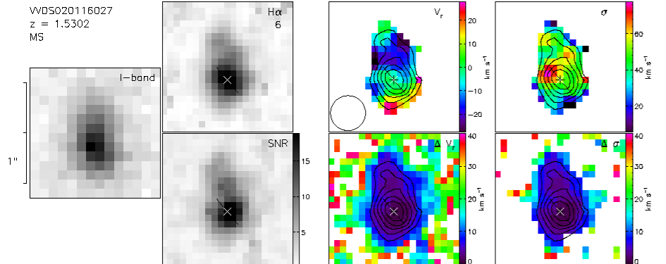
Figure 14: VVDS020116027 maps. From left to right: $I$-band CFHT legacy survey best seeing image, H$\alpha$ flux (top) and signal-to-noise (bottom) maps, H$\alpha$ velocity field (top) and associated errors (bottom), H$\alpha$ velocity dispersion map and associated errors (bottom) obtained from Gaussian fits to the SINFONI data cubes after smoothing spatially with a two-dimensional Gaussian of FWHM $=$ 2 pixels. Except the instrumental spectral PSF, no correction has been applied to compute the velocity dispersion map. Kinematical maps have been masked using the following criteria: (i) the line width must be larger than the one of the spectral PSF (the majority white pixels in the velocity dispersion error map), (ii) the uncertainty on the velocity must be less than 30 $km\leavevmode\nobreak\ s^{-1}$ and (iii) the signal-to-noise ratio larger than $\sim 2$. The $I$-band image and H$\alpha$ maps are color-coded with a linear scaling such that the values increase from light to dark. The integrated H$\alpha$ flux is quoted in each H$\alpha$ flux map in $10^{-17}$ergs s^-1 cm^-2. In error maps, values larger than the scale maximum are displayed using white. The angular size is indicated and the final seeing FWHM (including observational seeing and gaussian smoothing) is plotted as a circle on the velocity field. North is up, East is left. The center used for kinematical analysis is marked on each kinematical map with a black and white double cross. The solid line represents the orientation of the kinematical major axis and ends at half light radius measured on I-band images. The flux contours are overplotted on the velocity field, the velocity dispersion map and their associated error maps. The redshift derived from SINFONI data and the dynamical classification are quoted (RD for rotating disks, PR for perturbed rotators, MS for merging systems).

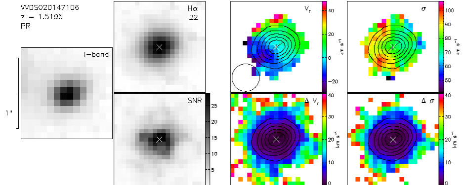
Figure 16: Similar as Figure 14 for VVDS020147106.

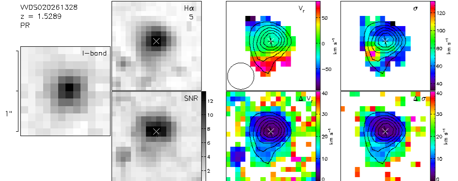
Figure 17: Similar as Figure 14 for VVDS020261328. The East feature in the signal-to-noise map correspond to a badly subtracted cosmic ray.

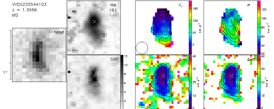
Figure 20: Similar as Figure 18 for VVDS220544103.

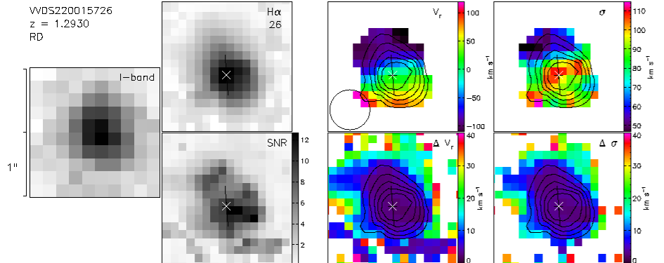
Figure 21: Similar as Figure 18 for VVDS220015726.

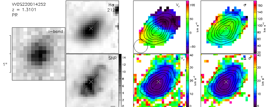
Figure 22: Similar as Figure 18 for VVDS220014252.

VVDS020116027

This galaxy shows a faint and irregular velocity gradient. The H$\alpha$ flux map, the velocity field and the velocity dispersion map suggest two components separated of about 6 kpc (0.75″). Indeed, the velocities decrease from South to North accross the main component but decrease of around 15 $km\leavevmode\nobreak\ s^{-1}$ when reaching the faint component. The separation between the two components is characterized by a higher velocity dispersion that could indicate a merging event (Amram et al. 2007) or an unresolved gap in velocity between the two components. The velocity separation of the centers of these two components is close to 0 $km\leavevmode\nobreak\ s^{-1}$. The merging timescale would be around 0.4 Gyr (from Kitzbichler & White 2008). The faint component is not seen in the $I$-band CFHTLS image, but the system appears as distorted and elongated, leading to an inclination of the whole system of 50^∘. The very low maximum rotation velocity (50 $km\leavevmode\nobreak\ s^{-1}$) may indicate that the object is almost not rotating ($V_{max}/\sigma_{0}=1.1$) or that the main component is seen nearly face-on. Fitting a rotating disk model for this system has been attempted both with or without masking the northern component. In both cases, a low $\chi^{2}$ is obtained but is due to the low velocities measured in this galaxy. The $\sigma$-peak around 70 $km\leavevmode\nobreak\ s^{-1}$ located at 0.3″ at the North-East of the maximum of the H$\alpha$ flux is not accounted for by these models. Due to both the low velocity dispersion and maximum rotation velocity, this object is one of the less massive of our sample ($5.5\times 10^{10}\,{\rm M_{\odot}}$). This object is classified as a major merger, presumably in a premerging state since the SFR_Hα is rather faint, indicating that the starburst event would not be yet engaged.

VVDS020182331

The flux of this galaxy is mostly concentrated in the central parts. This galaxy shows a perturbed velocity field. A strong sky line residual (14605Å) perturbs the line measurements and is responsible for both northern velocity dispersion and line flux peaks observed towards the North. The uncertainty on the velocity measurements is lower than 20 $km\leavevmode\nobreak\ s^{-1}$ for the central arcsecond only (in diameter). In this central part, a rotating disk model is acceptable. The corrected velocity dispersion of this object is high (71 $km\leavevmode\nobreak\ s^{-1}$). We do not detect in H$\alpha$ the close-by object revealed in CFHTLS best seeing images, indicating that this object is a foreground or background galaxy or that it is a companion with no star formation with which VVDS020182331 may interact. The latter explanation could explain the perturbed rotation observed in VVDS020182331. This object is slightly more rotation supported than dispersion supported ($V_{max}/\sigma_{0}=1.9$) and has a dynamical mass of $4.1\times 10^{10}\,{\rm M_{\odot}}$. It is classified as a perturbed rotator.

VVDS020147106

The H$\alpha$ flux is concentrated in the center. The size of the galaxy is twice the seeing (see Table 1). This galaxy shows a faint velocity shear compatible with a face-on rotating disk. The velocity dispersion map does not show any peak but is higher on the eastern side (of about 20 $km\leavevmode\nobreak\ s^{-1}$). The northern edge shows higher velocities of about 30 $km\leavevmode\nobreak\ s^{-1}$. However the one pixel crown of the edges has higher uncertainties due to a low signal to noise ratio (lower than 4) and was masked to fit a rotating disk model. The fit indicates that a low velocity plateau (30 $km\leavevmode\nobreak\ s^{-1}$) is reached close to the center. This low maximum rotation velocity suggests that the inclination of this system is even lower than suggested from the $I$-band image or that this object is strongly dispersion dominated ($V_{max}/\sigma_{0}=0.4$). Due to compactness of this object ($r_{1/2}=1.2$ kpc) and compared to the total extent of H$\alpha$ emission ($R_{last}=6.4$ kpc), the dispersion mass is estimated to $27.4\times 10^{10}\,{\rm M_{\odot}}$, which is 15 times larger than the stellar mass ($1.7\times 10^{10}\,{\rm M_{\odot}}$). This suggests that this star-forming galaxy is embedded in a large dark matter halo or that it contains a large amount of gas. Even if it can not be excluded that this galaxy is a dispersion dominated spheroid , this galaxy is classified as a perturbed rotating disk since it has a high velocity dispersion (80 $km\leavevmode\nobreak\ s^{-1}$) and shows rotation in its perturbed velocity field. The asymmetries observed in the velocity maps could be accounted for by a minor merging event.

VVDS020261328

The H$\alpha$ flux map is peaked and faintly extends toward the South. The velocity dispersion map has a peak around 120 $km\leavevmode\nobreak\ s^{-1}$ in the South-East. The velocity field shows a clear but irregular velocity shear of about 100 $km\leavevmode\nobreak\ s^{-1}$ that extends over 0.8″ in radius. Fitting a rotating disk model suggests that only the central part of the galaxy is detected since the plateau is not reached. It also shows that the velocity dispersion peak cannot be explained by the beam smearing effects. For the same reasons as VVDS020147106, VVDS020261328 has a dynamical mass ($19.6\times 10^{10}\,{\rm M_{\odot}}$) 30 times larger than the stellar mass ($0.6\times 10^{10}\,{\rm M_{\odot}}$) suggesting that dark matter and cool gas dominate the gravitational potential of this galaxy. The SFR is the lowest of our sample (see Table 3). This galaxy is classified as a pertubed rotator mainly rotation supported ($V_{max}/\sigma_{0}=3.5$).

VVDS220596913

The H$\alpha$ flux map shows two main components separated by 12.5 kpc (1.5″) that are not clearly distinguished in the $I$-band image. The brigthest component is located in the western side and is composed by two peaks of equal intensity. The eastern component is much fainter. It has a smooth velocity gradient and two peaks in the velocity dispersion map (around 100 $km\leavevmode\nobreak\ s^{-1}$). One corresponds to the brightest H$\alpha$ knot, and the other is more diffuse and corresponds to the transition region between the two components where the H$\alpha$ emission is the faintest (signal to noise ratio around 4). The high velocity dispersion between the two components can be a signature for merging as for Hickson compact group H31 (Amram et al. 2007). The velocity shear of the faint component is misaligned by around 20^∘ with respect to the one of the brigth component suggesting, as does the flux distribution, that this system is composed of two galaxies in the process of merging. The velocity separation of the two components is estimated to $\sim 150$ $km\leavevmode\nobreak\ s^{-1}$. The merging timescale would be around 1.2 Gyr. Although a large and unique rotating disk consituted by large clumps as seen in Bournaud et al. (2008) cannot be excluded (leading to $V_{max}/\sigma_{0}=2.3$), fitting the brightest component alone gives better results in terms of $\chi^{2}$, suggesting that the main component is rotating with a maximum velocity of around 200 $km\leavevmode\nobreak\ s^{-1}$. We fixed the center between the two flux peaks of the main component, and used an inclination of $55$^∘. Assuming that both components have the same dimensions (half the whole system dimensions), we obtained a dynamical mass of around $8\pm 2\times 10^{10}\,{\rm M_{\odot}}$ (dominated by rotation) for the bright component and $4\pm 2\times 10^{10}\,{\rm M_{\odot}}$ (dominated by dispersion) for the faint one. This imply a total dynamical mass of $\sim 12\times 10^{10}\,{\rm M_{\odot}}$ of the same order as the one computed considering a unique object ($\sim 13\times 10^{10}\,{\rm M_{\odot}}$). This object is classified as a major merger system.

VVDS220584167

VVDS220584167 is the object that presents the most extended H$\alpha$ map of the sample. It has an elongated peak in the velocity dispersion map close to the center. The observation is affected by a strong sky line residual (16195Å, see Figure 8) that induces large uncertainties on line measurements, mainly on the southern side. The velocity field shows asymmetry and the galaxy presents a distorted morphology in the $I$-band image which makes possible the existence of a strong bar (see for comparison UGC 08937 in Epinat et al. 2009). Moreover, the observed displacement between $I$-band and H$\alpha$ morphologies suggests a violent star formation event compatible with the high SFR of this galaxy. The velocity field is reasonnably fit by a simple rotational disk model, and the central velocity dispersion peak is not accounted for by the model since it does not simulate the effect of a bar. VVDS220584167 is the most massive disk of the sample with a dynamical mass of $21.1\times 10^{10}\,{\rm M_{\odot}}$. It is also the most rotation-dominated object ($M_{\theta}/M_{\sigma}=18$ and $V_{max}/\sigma_{0}=5.9$). Thus this galaxy is classified as a rotating disk with a bar.

VVDS220544103

The H$\alpha$ flux map of VVDS220544103 shows two peaks separated by around 6 kpc (0.75″). It also shows a distorted morphology both in the line flux map and in the $I$-band image. A faint velocity gradient ($\sim 30$ $km\leavevmode\nobreak\ s^{-1}$) is observed toward the main northern peak, whereas a strong velocity gradient ($\sim 120$ $km\leavevmode\nobreak\ s^{-1}$) is observed at the South of the fainter southern peak. The two gradients are in the same direction and the velocity field is continuous accross the whole object. The isovelocities contours are perpendicular to the distorted and elongated morphology. The strongest peaks in the velocity dispersion are located at the edges where the signal to noise ratio is low. Excluding these peaks, the velocity dispersion map shows an elongated peak close to the faint H$\alpha$ flux peak. Fitting a simple rotating disk model to the whole system leads to a ratio $V_{max}/\sigma_{0}=2.1$. However, this object is hard to fit with such a model and the dynamical mass estimates just give an indication on its total mass. From our data, it is not possible to separate two components and compute mass estimates for both. We estimated the total dynamical mass to $10.3\times 10^{10}\,{\rm M_{\odot}}$ using a unique rotating disk object hypothesis. However, one might guess that at least one component could be seen nearly face-on and thus have a larger maximum velocity and thus a larger total mass. The velocity separation between the two components is around 40 $km\leavevmode\nobreak\ s^{-1}$. The merging timescale for this system would be around 0.5 Gyr. This object could be two or more galaxies in a merging process and is classified as a merging system.

VVDS220015726

The central regions give a clean signal, while the low signal regions are affected by sky residuals due to the proximity of two strong sky lines next to H$\alpha$ (15053Åand 15056Å). The H$\alpha$ map is peaked at the center and it has also a peak at the same location in the velocity dispersion map ($\sim 100$ $km\leavevmode\nobreak\ s^{-1}$). The kinematical maps of this galaxy are well reproduced by the rotating disk model. In particular, this model shows that the central velocity dispersion is due to beam smearing effects (see Figure 11). The relatively high $\chi^{2}$ value of the fit is only due to the fact that this object shows the highest velocities. VVDS220015726 is clearly dominated by rotation ($V_{max}/\sigma_{0}=8.5$) since it is the fastest rotator of the sample ($V_{max}=323$ $km\leavevmode\nobreak\ s^{-1}$) but also the object with the lowest velocity dispersion ($\sigma_{0}=38$ $km\leavevmode\nobreak\ s^{-1}$). Its total dynamical mass ($16.7\times 10^{10}\,{\rm M_{\odot}}$) is compatible within the error bars to its stellar mass ($6.2\times 10^{10}\,{\rm M_{\odot}}$). This indicates that the halo contribution is low in the central parts of this galaxy. This object is classified as a rotating disk.

VVDS220014252

The H$\alpha$ flux map of VVDS220014252 shows an elongated peak and diffuse emission in the outer parts, compatible with the $I$-band morphology. The peak does not perfectly match the center of external isophotes. The H$\alpha$ flux map also suggests the presence of an arm in the western side. The velocity field is the one of a rotating disk except in the eastern side where it shows unexpected high velocities. A rotating disk model correctly fits the velocity field. The fit is better (smaller $\chi^{2}$) when the center does not match the H$\alpha$ flux peak, but the center of external isophotes. Adopting an inclination of 56^∘, the deprojected maximum rotation velocity is quite low (103 $km\leavevmode\nobreak\ s^{-1}$). The model shows that the maximum rotation velocity is reached close to the kinematical center. The North-West side of the velocity field shows a bump and thus a small decrease. Around this bump, profiles are broad and asymmetric. Broad profiles (more than 150 $km\leavevmode\nobreak\ s^{-1}$) are also observed at the North-East edge, with a rather good signal to noise ratio (larger than 5). The velocity dispersion is not peaked at the center of the galaxy but is high everywhere. Moreover, the mean velocity dispersion of this galaxy is the highest of the whole sample (92 $km\leavevmode\nobreak\ s^{-1}$). The model shows that the velocity dispersion is not due to beam smearing effects (see Figure 11). The broad and asymmetric profiles suggests the possibility to have intrinsic double profiles that can be signatures of interactions (Amram et al. 2007). Moreover, the kinematics is not dominated by rotation since $V_{max}/\sigma_{0}=1.1$ and the total dynamical mass ($10.2\times 10^{10}\,{\rm M_{\odot}}$) is dominated by the dispersion mass ($7.9\times 10^{10}\,{\rm M_{\odot}}$). For these reasons, this galaxy showing the highest SFR of the sample is classified as a perturbed rotator possibly in the process of a minor merging event.