Sparse Regression Learning by Aggregation and Langevin Monte-Carlo

Abstract

We consider the problem of regression learning for deterministic design and independent random errors. We start by proving a sharp PAC-Bayesian type bound for the exponentially weighted aggregate (EWA) under the expected squared empirical loss. For a broad class of noise distributions the presented bound is valid whenever the temperature parameter $\beta$ of the EWA is larger than or equal to $4\sigma^{2}$, where $\sigma^{2}$ is the noise variance. A remarkable feature of this result is that it is valid even for unbounded regression functions and the choice of the temperature parameter depends exclusively on the noise level.

Next, we apply this general bound to the problem of aggregating the elements of a finite-dimensional linear space spanned by a dictionary of functions $\phi_{1},\ldots,\phi_{M}$. We allow $M$ to be much larger than the sample size $n$ but we assume that the true regression function can be well approximated by a sparse linear combination of functions $\phi_{j}$. Under this sparsity scenario, we propose an EWA with a heavy tailed prior and we show that it satisfies a sparsity oracle inequality with leading constant one.

Finally, we propose several Langevin Monte-Carlo algorithms to approximately compute such an EWA when the number $M$ of aggregated functions can be large. We discuss in some detail the convergence of these algorithms and present numerical experiments that confirm our theoretical findings.

1 Introduction

In recent years a great deal of attention has been devoted to learning in high-dimensional models under the sparsity scenario. This typically assumes that, in addition to the sample, we have a finite dictionary of very large cardinality such that a small set of its elements provides a nearly complete description of the underlying model. Here, the words “large” and “small” are understood in comparison with the sample size. Sparse learning methods have been successfully applied in bioinformatics, financial engineering, image processing, etc. (see, e.g., the survey in [44]).

A popular model in this context is linear regression. We observe $n$ pairs $({\boldsymbol{X}}_{1},Y_{1}),\ldots,({\boldsymbol{X}}_{n},Y_{n})$, where each ${\boldsymbol{X}}_{i}$ – called the predictor – belongs to ${\mathbb{R}}^{M}$ and $Y_{i}$ – called the response – is scalar and satisfies $Y_{i}={\boldsymbol{X}}_{i}^{\top}{\boldsymbol{\lambda}}_{0}+\xi_{i}$ with some zero-mean noise $\xi_{i}$. The goal is to develop inference on the unknown vector ${\boldsymbol{\lambda}}_{0}\in{\mathbb{R}}^{M}$.

In many applications of linear regression the dimension of ${\boldsymbol{X}}_{i}$ is much larger than the sample size, i.e., $M\gg n$. It is well-known that in this case classical procedures, such as the least squares estimator, do not work. One of the most compelling ways for dealing with the situation where $M\gg n$ is to suppose that the sparsity assumption is fulfilled, i.e., that ${\boldsymbol{\lambda}}_{0}$ has only few coordinates different from $0$. This assumption is helpful at least for two reasons: The model becomes easier to interpret and the consistent estimation of ${\boldsymbol{\lambda}}_{0}$ becomes possible if the number of non-zero coordinates is small enough.

During the last decade several learning methods exploiting the sparsity assumption have been discussed in the literature. The $\ell_{1}$-penalized least squares (Lasso) is by far the most studied one and its statistical properties are now well understood (cf., e.g., [4, 6, 7, 5, 31, 39, 45] and the references cited therein). The Lasso is particularly attractive by its low computational cost. For instance, one can use the LARS algorithm [19], which is quite popular. Other procedures based on closely related ideas include the Elastic Net [47], the Dantzig selector [9] and the least squares with entropy penalization [27]. However, one important limitation of these procedures is that they are provably consistent under rather restrictive assumptions on the Gram matrix associated to the predictors, such as the mutual coherence assumption [18], the uniform uncertainty principle [8], the irrepresentable [46] or the restricted eigenvalue [4] conditions. This is somewhat unsatisfactory, since it is known that, at least in theory, there exist estimators attaining optimal accuracy of prediction under almost no assumption on the Gram matrix. This is, in particular, the case for the $\ell_{0}$-penalized least squares estimator [7, Thm. 3.1]. However, the computation of this estimator is an NP-hard problem. We finally mention the paper [42], which brings to attention the fact that the empirical Bayes estimator in Gaussian regression with Gaussian prior can effectively recover the sparsity pattern. This method is realized in [42] via the EM algorithm. However, its theoretical properties are not explored, and it is not clear what are the limits of application of the method beyond the considered set of numerical examples.

In [15, 16] we proposed another approach to learning under the sparsity scenario, which consists in using an exponentially weighted aggregate (EWA) with a properly chosen sparsity-favoring prior. There exists an extensive literature on EWA. Some recent results focusing on the statistical properties can be found in [2, 3, 11, 24, 28, 43]. Application of EWA to the single-index regression and Gaussian graphical models has been developed in [20] and [21], respectively. Procedures with exponential weighting received much attention in the literature on the on-line learning, see [12, 22, 40], the monograph [14] and the references cited therein.

The main message of [15, 16] is that the EWA with a properly chosen prior is able to deal with the sparsity issue. In particular, [15, 16] prove that such an EWA satisfies a sparsity oracle inequality (SOI), which is more powerful than the best known SOI for other common procedures of sparse recovery. An important point is that almost no assumption on the Gram matrix is required. In the present work we extend this analysis in two directions. First, we prove a sharp PAC-Bayesian bound for a large class of noise distributions, which is valid for the temperature parameter depending only on the noise distribution. We impose no restriction on the values of the regression function. This result is presented in Section 2. The consequences in the context of linear regression under sparsity assumption are discussed in Section 3.

The second problem that we analyze here is the computation of EWA with the sparsity prior. Since we want to deal with large dimensions $M$, computation of integrals over ${\mathbb{R}}^{M}$ in the definition of this estimator can be a hard problem. Therefore, we suggest an approximation based on Langevin Monte-Carlo (LMC). This is described in detail in Section 4. Section 5 contains numerical experiments that confirm fast convergence properties of the LMC and demonstrate a nice performance of the resulting estimators.

2 PAC-Bayesian type oracle inequality

Throughout this section, as well as in Section 3, we assume that we are given the data $(Z_{i},Y_{i}),\,i=1,\ldots,n$, generated by the non-parametric regression model

$$Y_{i}=f(Z_{i})+\xi_{i},\qquad i=1,\ldots,n,$$ (1)

with deterministic design $Z_{1},\ldots,Z_{n}$ and random errors $\xi_{i}$. We use the vector notation ${\mathbf{Y}}=\boldsymbol{f}+{\boldsymbol{\xi}}$, where ${\boldsymbol{\xi}}=(\xi_{1},\dots,\xi_{n})^{\top}$ and the function $f(\cdot)$ is identified with the vector $\boldsymbol{f}=(f(Z_{1}),\ldots,f(Z_{n}))^{\top}$. The space $\mathcal{Z}$ containing the design points $Z_{i}$ can be arbitrary and $f$ is a mapping from $\mathcal{Z}$ to ${\mathbb{R}}$. For each function $h:\mathcal{Z}\to{\mathbb{R}}$, we denote by $\|h\|_{n}$ the empirical norm $\big{(}\frac{1}{n}\sum_{i=1}^{n}h(Z_{i})^{2}\big{)}^{1/2}$. Along with these notation, we will denote by $\|{\boldsymbol{v}}\|_{p}$ the $\ell_{p}$-norm of a vector ${\boldsymbol{v}}=(v_{1},\dots,v_{n})\in{\mathbb{R}}^{n}$, that is $\|{\boldsymbol{v}}\|_{p}^{p}=\sum_{i=1}^{n}|v_{i}|^{p}$, $1\leqslant p<\infty$, $\|{\boldsymbol{v}}\|_{\infty}=\max_{i}|v_{i}|$ and $\|{\boldsymbol{v}}\|_{0}$ is the number of nonzero entries of ${\boldsymbol{v}}$. With this notation, $\|\boldsymbol{f}\|_{2}^{2}=n\|f\|_{n}^{2}$.

Assume that we are given a collection $\{f_{\lambda}:\lambda\in\Lambda\}$ of functions $f_{\lambda}:\mathcal{Z}\to{\mathbb{R}}$ that will serve as building blocks for the learning procedure.The set $\Lambda$ is assumed to be equipped with a $\sigma$-algebra and the mappings $\lambda\mapsto f_{\lambda}(z)$ are assumed to be measurable with respect to this $\sigma$-algebra for all $z\in\mathcal{Z}$. Let $\pi$ be a probability measure on $\Lambda$, called the prior, and let $\beta$ be a positive real number, called the temperature parameter. We define the EWA by

$$\widehat{f}_{n}(z)=\int_{\Lambda}f_{\lambda}(z)\,\widehat{\pi}_{n,\beta}(d\lambda),$$

where $\widehat{\pi}_{n,\beta}$ is the (posterior) probability distribution

$$\widehat{\pi}_{n,\beta}(d\lambda)\propto\exp\big{\{}-\beta^{-1}\|{\mathbf{Y}}-\boldsymbol{f}_{\lambda}\|_{2}^{2}\big{\}}\,\pi(d\lambda),$$

and $\boldsymbol{f}_{\lambda}=(f_{\lambda}(Z_{1}),\ldots,f_{\lambda}(Z_{n}))^{\top}$. We denote by $L$ the smallest positive number, which may be equal to $+\infty$, such that

$$(\lambda,\lambda^{\prime})\in\Lambda^{2}\quad\Longrightarrow\quad\max_{i}|f_{\lambda}(Z_{i})-f_{\lambda^{\prime}}(Z_{i})|\leqslant L$$ (2)

In the sequel, we use the convention $\frac{+\infty}{+\infty}=0$ and, for any function $v:{\mathbb{R}}\to{\mathbb{R}}$, we denote by $\|v\|_{\infty}$ its $L_{\infty}({\mathbb{R}})$-norm.

In order to get meaningful statistical results on the accuracy of the EWA, some conditions on the noise are imposed. In addition to the standard assumptions that the noise vector ${\boldsymbol{\xi}}=(\xi_{1},\ldots,\xi_{n})^{\top}$ has zero mean and independent identically distributed (iid) coordinates, we require the following assumption on the distribution of $\xi_{1}$.

Assumption N. For any $\gamma>0$ small enough, there exist a probability space and two random variables $\xi$ and $\zeta$ defined on this probability space such that

• $\xi$ has the same distribution as the regression errors $\xi_{i}$,
  

• $\xi+\zeta$ has the same distribution as $(1+\gamma)\xi$ and the conditional expectation satisfies $\mathbf{E}[\zeta\,|\,\xi]=0$,
  

• there exist $t_{0}\in(0,\infty]$ and a bounded Borel function $v:{\mathbb{R}}\to{\mathbb{R}}_{+}$ such that

  $$\varlimsup_{\gamma\to 0}\ \sup_{(t,a)\in[-t_{0},t_{0}]\times{\rm supp}(\xi)}\frac{\log\mathbf{E}[e^{t\zeta}\,|\,\xi=a]}{t^{2}\gamma v(a)}\leqslant 1,$$

  where ${\rm supp}(\xi)$ is the support of the distribution of $\xi$.

Many symmetric distributions used in applications satisfy Assumption N with functions $v$ such that $\|v\|_{\infty}$ is a multiple of the variance of the noise $\xi_{i}$. This follows from Remarks 1-6 given at the end of this section and their combinations.

Theorem 1.

Let Assumption N be satisfied with some function $v$ and let (2) hold. Then for any prior $\pi$, any probability measure $p$ on $\Lambda$ and any $\beta\geqslant\max(4\|v\|_{\infty},2L/t_{0})$ we have

$$\mathbf{E}[\|\widehat{f}_{n}-f\|_{n}^{2}]\leqslant\int_{\Lambda}\|f-f_{\lambda}\|_{n}^{2}\,p(d\lambda)+\frac{\beta\mathcal{K}(p,\pi)}{n},$$

where $\mathcal{K}(\cdot\,,\cdot\;\!)$ stands for the Kullback-Leibler divergence.

Prior to presenting the proof, let us note that Theorem 1 is in the spirit of [16, Theorems 1,2], but is better in several aspects. First, the main assumption ensuring the validity of the oracle inequality involves the distribution of the noise alone, while [16, Theorem 2] relies on an assumption (denoted by (C) in [16]) that ties together the distributional properties of the noise and the nature of the dictionary $\{f_{\lambda}\}$. A second advantage is that Assumption N is independent of the sample size $n$ and, consequently, suggests a choice of the parameter $\beta$ that does not change with the sample size. Theorem 1 of [16] also has these advantages but it is valid only for a very restricted class of noise distributions, essentially for the Gaussian and uniform noise. As we shall see later in this section, Theorem 1 leads to a choice of the tuning parameter $\beta$, which is very simple and guarantees the validity of a strong oracle inequality for a large class of noise distributions.

Proof of Theorem 1.

It suffices to prove the theorem for $p$ such that $\int_{\Lambda}\|f_{\lambda}-f\|_{n}^{2}\,p(d\lambda)<\infty$ and $p\ll\pi$ (implying $\mathcal{K}(p,\pi)<\infty$), since otherwise the result is trivial.

We first assume that $\beta>4\|v\|_{\infty}$ and that $L<\infty$. Let $\gamma>0$ be a small number. Let now $(\xi_{1},\zeta_{1}),\ldots,(\xi_{n},\zeta_{n})$ be a sequence of iid pairs of random variables defined on a common probability space such that $(\xi_{i},\zeta_{i})$ satisfy conditions i)-iii) of Assumption N for any $i$. The existence of these random variables is ensured by Assumption N. We use here the same notation $\xi_{i}$ as in model (1), since it causes no ambiguity.

Set ${\boldsymbol{h}}_{\lambda}=f_{\lambda}-f$, $\widehat{h}=\widehat{f}_{n}-f$, ${\boldsymbol{\zeta}}=(\zeta_{1},\dots,\zeta_{n})^{\top}$, $U({\boldsymbol{h}},{\boldsymbol{h}}^{\prime})=\|{\boldsymbol{h}}\|_{2}^{2}+2{{\boldsymbol{h}}\!}^{\top}{\boldsymbol{h}}^{\prime}$ and $\Delta U({\boldsymbol{h}},{\boldsymbol{h}}^{\prime},{\boldsymbol{h}}^{\prime\prime})=(\|{\boldsymbol{h}}\|_{2}^{2}-\|{\boldsymbol{h}}^{\prime}\|_{2}^{2})+2({\boldsymbol{h}}-{\boldsymbol{h}}^{\prime})^{\top}{\boldsymbol{h}}^{\prime\prime}$ for any pair ${\boldsymbol{h}},{\boldsymbol{h}}^{\prime},{\boldsymbol{h}}^{\prime\prime}\in{\mathbb{R}}^{n}$. With this notation we have

$$\mathbf{E}[\|\widehat{f}_{n}-f\|_{n}^{2}]=\mathbf{E}[\|\widehat{h}\|_{n}^{2}]=\mathbf{E}\Big{[}\|\widehat{h}\|_{n}^{2}+\frac{2}{n\gamma}\widehat{\boldsymbol{h}}^{\top}\!{\boldsymbol{\zeta}}\Big{]}.$$

Therefore, $\mathbf{E}[\|\widehat{f}_{n}-f\|_{n}^{2}]=S+S_{1}$, where

$$S\!\!\!\! = \!\!\!-\frac{\beta}{n\gamma}\mathbf{E}\Big{[}\log\int_{\Lambda}\exp\!\Big{(}\!-\frac{\gamma U({\boldsymbol{h}}_{\lambda},\gamma^{-1}{\boldsymbol{\zeta}})}{\beta}\Big{)}\,\widehat{\pi}_{n,\beta}(d\lambda)\Big{]},$$

$$S_{1}\!\!\!\!\! = \!\!\!\frac{\beta}{n\gamma}\mathbf{E}\Big{[}\log\!\!\int_{\Lambda}\exp\!\Big{(}\!-\frac{\gamma\Delta U({\boldsymbol{h}}_{\lambda},\widehat{\boldsymbol{h}},\gamma^{-1}{\boldsymbol{\zeta}})}{\beta}\Big{)}\,\widehat{\pi}_{n,\beta}(d\lambda)\Big{]}.$$

We first bound the term $S$. To this end, note that

$$\widehat{\pi}_{n,\beta}(d\lambda)=\frac{\exp\{-\beta^{-1}U({\boldsymbol{h}}_{\lambda},{\boldsymbol{\xi}})\}}{\int_{\Lambda}\exp\{-\beta^{-1}U({\boldsymbol{h}}_{w},{\boldsymbol{\xi}})\}\pi(dw)}\;\pi(d\lambda)$$

and, therefore,

$$S\!\!\! = \!\!\!\frac{\beta}{n\gamma}\mathbf{E}\Big{[}\!\log\int_{\Lambda}\exp\big{\{}\!\!-\hbox{$\frac{1}{\beta}$}U({\boldsymbol{h}}_{\lambda},{\boldsymbol{\xi}})\big{\}}\pi(d\lambda)\Big{]}-\frac{\beta}{n\gamma}\mathbf{E}\Big{[}\!\log\!\int_{\Lambda}\!\exp\big{\{}-\hbox{$\frac{1+\gamma}{\beta}$}U\big{(}{\boldsymbol{h}}_{\lambda},\hbox{$\frac{{\boldsymbol{\xi}}+{\boldsymbol{\zeta}}}{1+\gamma}$}\big{)}\big{\}}\pi(d\lambda)\Big{]}.$$

By part ii) of Assumption N and the independence of vectors $(\xi_{i},\zeta_{i})$ for different values of $i$, the probability distribution of the vector $({\boldsymbol{\xi}}+{\boldsymbol{\zeta}})/(1+\gamma)$ coincides with that of ${\boldsymbol{\xi}}$. Therefore, $({\boldsymbol{\xi}}+{\boldsymbol{\zeta}})/(1+\gamma)$ may be replaced by ${\boldsymbol{\xi}}$ inside the second expectation. Now, using the Hölder inequality, we get

$$S\!\!\!\! \leqslant \!\!\!\!-\frac{\beta}{n(1+\gamma)}\mathbf{E}\Big{[}\log\int_{\Lambda}e^{-(1+\gamma)\beta^{-1}U({\boldsymbol{h}}_{\lambda},{\boldsymbol{\xi}})}\pi(d\lambda)\Big{]}.$$

Next, by a convex duality argument [10, p. 160], we find

$$S\leqslant\int_{\Lambda}\|h_{\lambda}\|_{n}^{2}\,p(d\lambda)+\frac{\beta\mathcal{K}(p,\pi)}{n(1+\gamma)}\ .$$

Let us now bound the term $S_{1}$. According to part iii) of Assumption N, there exists $\gamma_{0}>0$ such that $\forall\gamma\leqslant\gamma_{0}$,

$$\sup_{|t|\leqslant t_{0}}\frac{\log\mathbf{E}[e^{t\zeta}|\xi=a]}{t^{2}\gamma}\leqslant v(a)(1+o_{\gamma}(1)),\quad\forall\,a\in{\mathbb{R}}.$$

In what follows we assume that $\gamma\leqslant\gamma_{0}$. Since for every $i$, $|2\beta^{-1}(h_{\lambda}(Z_{i})-\widehat{h}(Z_{i}))|\leqslant 2\beta^{-1}L\leqslant t_{0}$, using Jensen’s inequality we get

$$S_{1}\!\!\!\! \leqslant \!\!\!\!\frac{\beta}{n\gamma}\mathbf{E}\Big{[}\log\!\int_{\Lambda}\exp\Big{\{}-\frac{n\gamma}{\beta}(\|h_{\lambda}\|_{n}^{2}-\|\widehat{h}\|_{n}^{2})\Big{\}}\,\theta_{\lambda}\,\mathbf{E}\!\Big{(}\!\exp\!\Big{\{}\!\sum_{i=1}^{n}2\beta^{-1}(h_{\lambda}(Z_{i})-\widehat{h}(Z_{i}))\zeta_{i}\!\Big{\}}\big{|}{{\boldsymbol{\xi}}}\Big{)}\pi(d\lambda)\Big{]}$$

$$\leqslant \!\!\!\!\frac{\beta}{n\gamma}\mathbf{E}\Big{[}\log\!\int_{\Lambda}\exp\Big{\{}-\frac{n\gamma}{\beta}(\|h_{\lambda}\|_{n}^{2}-\|\widehat{h}\|_{n}^{2})\Big{\}}\,\theta_{\lambda}\,\exp\Big{\{}\frac{4n\|v\|_{\infty}\gamma}{\beta^{2}}\|h_{\lambda}-\widehat{h}\|^{2}_{n}(1\!+o_{\gamma}(1))\Big{\}}\,\pi(d\lambda)\Big{]}.$$

For $\gamma$ small enough ($\gamma\leqslant\tilde{\gamma}_{0}$), this entails that up to a positive multiplicative constant, the term $S_{1}$ is bounded by the expression $\mathbf{E}\big{[}\log\int_{\Lambda}\exp\big{(}-\frac{n\gamma{V}(h_{\lambda},\widehat{h})}{\beta^{2}}\big{)}\theta_{\lambda}\pi(d\lambda)\big{]}$, where

$$V(h_{\lambda},\widehat{h})\!=\beta(\|h_{\lambda}\|_{n}^{2}-\|\widehat{h}\|_{n}^{2})\!+\frac{(\beta+4\|v\|_{\infty})}{2}\|h_{\lambda}\!-\widehat{h}\|^{2}_{n}.$$

Using [15, Lemma 3] and Jensen’s inequality we obtain $S_{1}\leqslant 0$ for any $\gamma\leqslant(\beta-4\|v\|_{\infty})/4nL$. Thus, we proved that

$$\mathbf{E}[\|\widehat{h}\|_{n}^{2}]\leqslant\int_{\Lambda}\|h_{\lambda}\|_{n}^{2}\,p\,(d\lambda)+\frac{\beta\,\mathcal{K}(p,\pi)}{n(1+\gamma)}$$

for any $\gamma\leqslant\tilde{\gamma}_{0}\wedge(\beta-4\|v\|_{\infty})/4nL$. Letting $\gamma$ tend to zero, we obtain

$$\mathbf{E}[\|\widehat{h}\|_{n}^{2}]\leqslant\int_{\Lambda}\|h_{\lambda}\|_{n}^{2}p(d\lambda)+\frac{\beta\,\mathcal{K}(p,\pi)}{n}$$

for any $\beta>\max(4\|v\|_{\infty},2L/t_{0})$. Fatou’s lemma allows us to extend this inequality to the case $\beta=\max(4\|v\|_{\infty},2L/t_{0})$.

To cover the case $L=+\infty,t_{0}=+\infty$, we fix some $L_{0}\in(0,\infty)$ and apply the obtained inequality to the truncated prior $\pi^{L^{\prime}}(d\lambda)\propto{\rm 1}\mskip-4.5mu{\rm l}_{\Lambda_{L^{\prime}}}(\lambda)\pi(d\lambda)$, where $L^{\prime}\in(L_{0},\infty)$ and $\Lambda_{L^{\prime}}=\{\lambda\in\Lambda:\max_{i}|f_{\lambda}(Z_{i})|\leqslant L^{\prime}\}$. We obtain that for any measure $p\ll\pi$ supported by $\Lambda_{L_{0}}$,

$$\mathbf{E}[\|\widehat{h}^{L^{\prime}}\|_{n}^{2}]\!\!\!\! \leqslant \!\!\!\!\int_{\Lambda}\|h_{\lambda}\|_{n}^{2}\,p(d\lambda)+\frac{\beta\mathcal{K}(p,\pi^{L^{\prime}})}{n}$$

$$\leqslant \!\!\!\!\int_{\Lambda}\|h_{\lambda}\|_{n}^{2}\,p(d\lambda)+\frac{\beta\mathcal{K}(p,\pi)}{n}.$$

One easily checks that $\widehat{h}^{L^{\prime}}$ tends a.s. to $\widehat{h}$ and that the random variable $\sup_{L^{\prime}>L_{0}}\|\widehat{h}^{L^{\prime}}\|_{n}^{2}{\rm 1}\mskip-4.5mu{\rm l}(\max_{i}|\xi_{i}|\leqslant C)$ is integrable for any fixed $C$. Therefore, by Lebesgue’s dominated convergence theorem we get

$$\mathbf{E}[\|\widehat{h}\|_{n}^{2}{\rm 1}\mskip-4.5mu{\rm l}(\max_{i}|\xi_{i}|\leqslant C)]\!\!\!\! \leqslant \!\!\!\!\int_{\Lambda}\|h_{\lambda}\|_{n}^{2}\,p(d\lambda)+\frac{\beta\mathcal{K}(p,\pi)}{n}.$$

Letting $C$ tend to infinity and using Lebesgue’s monotone convergence theorem we obtain the desired inequality for any probability measure $p$ which is absolutely continuous w.r.t. $\pi$ and is supported by $\Lambda_{L_{0}}$ for some $L_{0}>0$. If $p(\Lambda_{L_{0}})<1$ for any $L_{0}>0$, one can replace $p$ by its truncated version $p^{L^{\prime}}$ and use Lebesgue’s monotone convergence theorem to get the desired result. ∎

The following remarks provide examples of noise distributions, for which Assumption N is satisfied. Proofs of these remarks are given in the Appendix.

Remark 1 (Gaussian noise).

If $\xi_{1}$ is drawn according to the Gaussian distribution $\mathcal{N}(0,\sigma^{2})$, then for any $\gamma>0$ one can choose $\zeta$ independently of $\xi$ according to the Gaussian distribution $\mathcal{N}(0,(2\gamma+\gamma^{2})\sigma^{2})$. This results in $v(a)\equiv\sigma^{2}$ and, as a consequence, Theorem 1 holds for any $\beta\geqslant 4\sigma^{2}$. Note that this reduces to the Leung and Barron’s [28] result if the prior $\pi$ is discrete.

Remark 2 (Rademacher noise).

If $\xi_{1}$ is drawn according to the Rademacher distribution, i.e. ${\mathbf{P}}(\xi_{1}=\pm\sigma)=1/2$, then for any $\gamma>0$ one can define $\zeta$ as follows:

$$\zeta=(1+\gamma)\sigma\mathop{\rm sgn}[\sigma^{-1}\xi-(1+\gamma)U]-\xi,$$

where $U$ is distributed uniformly in $[-1,1]$ and is independent of $\xi$. This results in $v(a)\equiv\sigma^{2}$ and, as a consequence, Theorem 1 holds for any $\beta\geqslant 4\sigma^{2}=4\mathbf{E}[\xi_{1}^{2}]$.

Remark 3 (Stability by convolution).

Assume that $\xi_{1}$ and $\xi_{1}^{\prime}$ are two independent random variables. If $\xi_{1}$ and $\xi_{1}^{\prime}$ satisfy Assumption N with $t_{0}=\infty$ and with functions $v(a)$ and $v^{\prime}(a)$, then any linear combination $\alpha\xi_{1}+\alpha^{\prime}\xi_{1}^{\prime}$ satisfies Assumption N with $t_{0}=\infty$ and the $v$-function $\alpha^{2}v(a)+(\alpha^{\prime})^{2}v^{\prime}(a)$.

Remark 4 (Uniform distribution).

The claim of preceding remark can be generalized to linear combinations of a countable set of random variables, provided that the series converges in the mean squared sense. In particular, if $\xi_{1}$ is drawn according to the symmetric uniform distribution with variance $\sigma^{2}$, then Assumption N is fulfilled with $t_{0}=\infty$ and $v(a)\equiv\sigma^{2}$. This can be proved using the fact that $\xi_{1}$ has the same distribution as $\sigma\sum_{i=1}^{\infty}2^{-i}\eta_{i}$, where $\eta_{i}$ are iid Rademacher random variables. Thus, in this case the inequality of Theorem 1 is true for any $\beta\geqslant 4\sigma^{2}$.

Remark 5 (Laplace noise).

If $\xi_{1}$ is drawn according to the Laplace distribution with variance $\sigma^{2}$, then for any $\gamma>0$ one can choose $\zeta$ independently of $\xi$ according to the distribution associated to the characteristic function

$$\varphi(t)=\frac{1}{(1+\gamma)^{2}}\Big{(}1+\frac{2\gamma+\gamma^{2}}{1+(1+\gamma)^{2}(\sigma t)^{2}/2}\Big{)}.$$

One can observe that the distribution of $\zeta$ is a mixture of the Dirac distribution at zero and the Laplace distribution with variance $(1+\gamma)^{2}\sigma^{2}$. This results in $v(a)\equiv 2\sigma^{2}/(2-\sigma^{2}t_{0}^{2})$ and, as a consequence, by taking $t_{0}=1/\sigma^{2}$, we get that Theorem 1 holds for any $\beta\geqslant\max(8\sigma^{2},2L\sigma)$.

Remark 6 (Bounded symmetric noise).

Assume that the errors $\xi_{i}$ are symmetric and that $P(|\xi_{i}|\leqslant B)=1$ for some $B\in(0,\infty)$. Let $U\sim\mathcal{U}([-1,1])$ be a random variable independent of $\xi$. Then, $\zeta=(1+\gamma)|\xi|\mathop{\rm sgn}[\mathop{\rm sgn}(\xi)-(1+\gamma)U]-\xi$ satisfies Assumption N with $v(a)=a^{2}$. Since $\|v\|_{\infty}\leqslant B^{2}$, we obtain that Theorem 1 is valid for any $\beta\geqslant 4B^{2}$.

Consider now the case of finite $\Lambda$. W.l.o.g. we suppose that $\Lambda=\{1,\dots,M\}$, $\{f_{\lambda},\lambda\in\Lambda\}=\{f_{1},\dots,f_{M}\}$ and we take the uniform prior $\pi(\lambda=j)=1/M$. From Theorem 1 we immediately get the following sharp oracle inequality for model selection type aggregation.

Corollary 1.

Let Assumption N be satisfied with some function $v$ and let (2) hold. Then for the uniform prior $\pi(\lambda=j)=1/M,j=1,\dots,M$, and any $\beta\geqslant\max(4\|v\|_{\infty},2L/t_{0})$ we have

$$\mathbf{E}[\|\widehat{f}_{n}-f\|_{n}^{2}]\leqslant\min_{j=1,\dots,M}\|f_{j}-f\|_{n}^{2}+\frac{\beta\log M}{n}.$$

This corollary can be compared with bounds for combining procedures in the theory of prediction of deterministic sequences [41, 29, 13, 26, 12, 14]. With our notation, the bounds proved in these works can be written is the form

$$\frac{1}{n}\sum_{i=1}^{n}(Y_{i}-f^{*}(Z_{i}))^{2}\leqslant C_{1}\min_{j=1,\dots,M}\frac{1}{n}\sum_{i=1}^{n}(Y_{i}-f_{j}(Z_{i}))^{2}+\frac{C_{2}\log M}{n}.$$ (3)

Here $f_{j}(Z_{i})$ is interpreted as the value of $Y_{i}$ predicted by the $j$th procedure, $f^{*}(Z_{i})$ as an aggregated forecast, and $C_{1}\geqslant 1$, $C_{2}>0$ are constants. Such inequalities are proved under the assumption that $Y_{i}$’s are deterministic and uniformly bounded. When $C_{1}=1$, applying (3) to random uniformly bounded $Y_{i}$’s from model (1) with $\mathbf{E}(\xi_{i})=0$ and taking expectations can yield an oracle inequality similar to that of Corollary 1. However, the uniform boundedness of $Y_{i}$’s supposes that not only the noise $\xi_{i}$ but also the functions $f$ and $f_{j}$ are uniformly bounded. Bounds on $f$ should be a priori known for the construction of the aggregated rule $f^{*}$ in (3) but in practice they are not always available. Our results are free of this drawback because they hold with no assumption on $f$. We have no assumption on the dictionary $\{f_{1},\dots,f_{M}\}$ neither.

3 Sparsity prior and SOI

In this section we introduce the sparsity prior and present a sparsity oracle inequality (SOI) derived from Theorem 1.

In what follows we assume that $\Lambda\subset{\mathbb{R}}^{M}$ for some positive integer $M$. We will use boldface letters to denote vectors and, in particular, the elements of $\Lambda$. For any square matrix A, let ${\rm Tr}(\textsf{A})$ denote the trace (sum of diagonal entries) of A. Furthermore, we focus on the particular case where $\mathcal{F}_{\Lambda}$ is the image of a convex polytope in ${\mathbb{R}}^{M}$ by a link function $g:{\mathbb{R}}\to{\mathbb{R}}$. More specifically, we assume that, for some $R\in(0,+\infty]$ and for a finite number of measurable functions $\big{\{}\phi_{j}\big{\}}_{j=1,\ldots,M}$,

$$\mathcal{F}_{\Lambda}=\Bigg{\{}f_{{\boldsymbol{\lambda}}}(z)=g\bigg{(}\sum_{j=1}^{M}\lambda_{\!j}\phi_{j}(z)\bigg{)},\ \forall z\in\mathcal{Z}\Big{|}\ {\boldsymbol{\lambda}}\in{\mathbb{R}}^{M}\text{ satisfies }\|{\boldsymbol{\lambda}}\|_{1}\leqslant R\,\Bigg{\}},$$

where $\|{\boldsymbol{\lambda}}\|_{1}=\sum_{j}|\lambda_{\!j}|$ stands for the $\ell_{1}$-norm. The link function $g$ is assumed twice continuously differentiable and known. Typical examples of link function include the linear function $g(x)=x$, the exponential function $g(x)=e^{x}$, the logistic function $g(x)=e^{x}/(e^{x}+1)$, the cumulative distribution function of the standard Gaussian distribution, and so on.

If, in addition, $f\in\mathcal{F}_{\Lambda}$, then model (1) reduces to that of single-index regression with known link function. In the particular case of $g(x)=x$, this leads to the linear regression defined in the Introduction. Indeed, it suffices to take

$${\boldsymbol{X}}_{i}=(\phi_{1}(Z_{i}),\ldots,\phi_{M}(Z_{i}))^{\top},\quad i=1,\ldots,n.$$

This notation will be used in the rest of the paper along with the assumption that ${\boldsymbol{X}}_{i}$ are normalized so that all the diagonal entries of matrix $\frac{1}{n}\sum_{i=1}^{n}{\boldsymbol{X}}_{i}{\boldsymbol{X}}_{i}^{\top}$ are equal to one.

The family $\mathcal{F}_{\Lambda}$ defined above satisfies inequality (2) with $L=2R\|g^{\prime}\|_{\infty}L_{\phi}$, where $L_{\phi}=\max_{i,j}|\phi_{j}(Z_{i})|$ and $\|g^{\prime}\|_{\infty}$ is the maximum of the derivative of $g$ on the interval $[-RL_{\phi},RL_{\phi}]$. Indeed, since $\Lambda$ is the $\ell_{1}$ ball of radius $R$ in ${\mathbb{R}}^{M}$ and $\phi_{j}$s are bounded by $L_{\phi}$, the real numbers $u_{i}={\boldsymbol{\lambda}}^{\top}{\boldsymbol{X}}_{i}$ and $u^{\prime}_{i}={{\boldsymbol{\lambda}}^{\prime}}^{\top}{\boldsymbol{X}}_{i}$ belong to the interval $[-RL_{\phi},RL_{\phi}]$ for every ${\boldsymbol{\lambda}}$ and ${\boldsymbol{\lambda}}^{\prime}$ from $\Lambda$. Consequently, $|f_{\boldsymbol{\lambda}}(Z_{i})-f_{{\boldsymbol{\lambda}}^{\prime}}(Z_{i})|=|g(u_{i})-g(u_{i}^{\prime})|=\int_{u_{i}}^{u_{i}^{\prime}}g^{\prime}(s)\,ds$ is bounded by $\|g^{\prime}\|_{\infty}|u_{i}-u_{i}^{\prime}|$, the latter being smaller than $2R\|g^{\prime}\|_{\infty}L_{\phi}$.

We allow $M$ to be large, possibly much larger than the sample size $n$. If $M\gg n$, we have in mind that the sparsity assumption holds, i.e., there exists ${{\boldsymbol{\lambda}}^{*}}\in{\mathbb{R}}^{M}$ such that $f$ in (1) is close to $f_{{{\boldsymbol{\lambda}}^{*}}}$ for some ${{\boldsymbol{\lambda}}^{*}}$ having only a small number of non-zero entries. We handle this situation via a suitable choice of prior $\pi$. Namely, we use a modification of the sparsity prior proposed in [15]. It should be emphasized right away that we will take advantage of sparsity for the purpose of prediction and not for data compression. In fact, even if the underlying model is sparse, we do not claim that our estimator is sparse as well, but we claim that it is quite accurate under very mild assumptions. On the other hand, some numerical experiments demonstrate the sparsity of our estimator and the fact that it recovers correctly the true sparsity pattern in examples where the (restrictive) assumptions mentioned in the Introduction are satisfied (cf. Section 5). However, our theoretical results do not deal with this property.

To specify the sparsity prior $\pi$ we need the Huber function $\bar{\omega}:{\mathbb{R}}\to{\mathbb{R}}$ defined by

$$\bar{\omega}(t)=\begin{cases}t^{2},&\text{ if }|t|\leqslant 1\\ 2|t|-1,&\text{ otherwise. }\end{cases}$$

This function behaves very much like the absolute value of $t$, but has the advantage of being differentiable at every point $t\in{\mathbb{R}}$. Let $\tau$ and $\alpha$ be positive numbers. We define the sparsity prior

$$\pi(d{\boldsymbol{\lambda}})=\frac{\tau^{2M}}{C_{\alpha,\tau,R}}\Bigg{\{}\prod_{j=1}^{M}\frac{e^{-\bar{\omega}(\alpha\lambda_{\!j})}}{(\tau^{2}+\lambda_{\!j}^{2})^{2}}\Bigg{\}}{\rm 1}\mskip-4.5mu{\rm l}(\|{\boldsymbol{\lambda}}\|_{1}\leqslant R)\,d{\boldsymbol{\lambda}},$$ (4)

where $C_{\alpha,\tau,R}$ is the normalizing constant.

Since the sparsity prior (4) looks somewhat complicated, an heuristical explanation is in order. Let us assume that $R$ is large and $\alpha$ is small so that the functions $e^{-\bar{\omega}(\alpha\lambda_{\!j})}$ and ${\rm 1}\mskip-4.5mu{\rm l}(\|{\boldsymbol{\lambda}}\|_{1}\leqslant R)$ are approximately equal to one. With this in mind, we can notice that $\pi$ is close to the distribution of $\sqrt{2}\tau{\mathbf{Y}}$, where ${\mathbf{Y}}$ is a random vector having iid coordinates drawn from Student’s t-distribution with three degrees of freedom. In the examples below we choose a very small $\tau$, smaller than $1/n$. Therefore, most of the coordinates of $\tau{\mathbf{Y}}$ are very close to zero. On the other hand, since Student’s t-distribution has heavy tails, a few coordinates of $\tau{\mathbf{Y}}$ are quite far from zero.

These heuristics are illustrated by Figure 1 presenting the boxplots of one realization of a random vector in ${\mathbb{R}}^{10.000}$ with iid coordinates drawn from the scaled Gaussian, Laplace (double exponential) and Student $t(3)$ distributions. The scaling factor is such that the probability densities of the simulated distributions are equal to $100$ at the origin. The boxplot which is most likely to represent a sparse vector corresponds to Student’s $t(3)$ distribution.

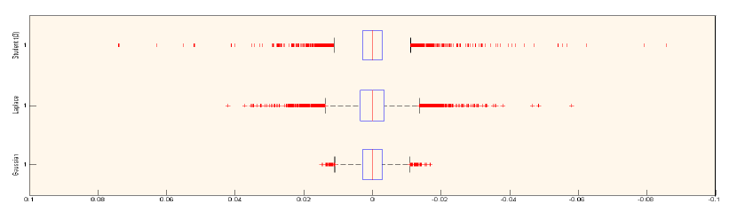
Figure 1: The boxplots of a sample of size $10^{4}$ drawn from the scaled Gaussian, Laplace and Student $t(3)$ distributions. In all the three cases the location parameter is $0$ and the scale parameter is $10^{-2}$.

The relevance of heavy tailed priors for dealing with sparsity has been emphasized by several authors (see [37, Section 2.1] and references therein). However, most of this work focused on logarithmically concave priors, such as the multivariate Laplace distribution. Also in wavelet estimation on classes of “sparse” functions [23] and [33] invoke quasi-Cauchy and Pareto priors. Bayes estimators with heavy-tailed priors in sparse Gaussian shift models are discussed in [1].

The next theorem provides a SOI for the EWA with the sparsity prior (4).

Theorem 2.

Let Assumption N be satisfied with some function $v$ and let (2) hold. Take the prior $\pi$ defined in (4) and $\beta\geqslant\max(4\|v\|_{\infty},2L/t_{0})$. Assume that $R>2M\tau$ and $\alpha\leqslant 1/(4M\tau)$. Then for all ${{\boldsymbol{\lambda}}^{*}}$ such that $\|{{\boldsymbol{\lambda}}^{*}}\|_{1}\leqslant R-2M\tau$ we have

$$\mathbf{E}[\|\widehat{f}_{n}-f\|_{n}^{2}]\!\!\!\! \leqslant \!\!\!\!\|f_{{{\boldsymbol{\lambda}}^{*}}}-f\|_{n}^{2}+\frac{4\beta}{n}\sum_{j=1}^{M}\log\big{(}1+\hbox{$\frac{|\lambda_{\!j}^{*}|}{\tau}$}\big{)}+\,\frac{2\beta(\alpha\|{{\boldsymbol{\lambda}}^{*}}\|_{1}+1)}{n}+4eC_{g,f}\tau^{2}M$$

with $C_{g,f}=1$ if $g(x)=x$ and $C_{g,f}=\|g^{\prime}\|_{\infty}^{2}+\|g^{\prime\prime}\|_{\infty}(\|g\|_{\infty}+\|f\|_{\infty})$ for other link functions $g$.

Proof.

Let us define the probability measure $p_{0}$ by

$$\frac{dp_{0}}{d{\boldsymbol{\lambda}}}({\boldsymbol{\lambda}})\propto\left(\frac{d\pi}{d{\boldsymbol{\lambda}}}({\boldsymbol{\lambda}}-{{\boldsymbol{\lambda}}^{*}})\right){\rm 1}\mskip-4.5mu{\rm l}_{B_{1}(2M\tau)}({\boldsymbol{\lambda}}-{{\boldsymbol{\lambda}}^{*}}).$$ (5)

Since $\|{{\boldsymbol{\lambda}}^{*}}\|_{1}\leqslant R-2M\tau$, the condition ${\boldsymbol{\lambda}}-{{\boldsymbol{\lambda}}^{*}}\in B_{1}(2M\tau)$ implies that ${\boldsymbol{\lambda}}\in B_{1}(R)$ and, therefore, $p_{0}$ is absolutely continuous w.r.t. the sparsity prior $\pi$. In view of Thm. 1, we have

$$\mathbf{E}[\|\widehat{f}_{n}-f\|^{2}_{n}]\leqslant\int_{\Lambda}\|f_{{\boldsymbol{\lambda}}}-f\|_{n}^{2}\,p_{0}(d{\boldsymbol{\lambda}})+\frac{\beta\mathcal{K}(p_{0},\pi)}{n}.$$

Since $f_{{\boldsymbol{\lambda}}}(Z_{i})=g({\boldsymbol{X}}_{i}^{\top}{\boldsymbol{\lambda}})$ we have $\nabla_{\boldsymbol{\lambda}}[(f_{{\boldsymbol{\lambda}}}(Z_{i})-f(Z_{i}))^{2}]=2g^{\prime}({\boldsymbol{X}}_{i}^{\top}{\boldsymbol{\lambda}})(f_{{\boldsymbol{\lambda}}}(Z_{i})-f(Z_{i})){\boldsymbol{X}}_{i}$ and

$$\nabla^{2}_{\boldsymbol{\lambda}}[(f_{{\boldsymbol{\lambda}}}(Z_{i})-f(Z_{i}))^{2}]=2\big{\{}g^{\prime}({\boldsymbol{X}}_{i}^{\top}{\boldsymbol{\lambda}})^{2}+g^{\prime\prime}({\boldsymbol{X}}_{i}^{\top}{\boldsymbol{\lambda}})\big{(}g({\boldsymbol{X}}_{i}^{\top}{\boldsymbol{\lambda}})-f(Z_{i})\big{)}\big{\}}{\boldsymbol{X}}_{i}{\boldsymbol{X}}_{i}^{\top}.$$

One can remark that the factor of ${\boldsymbol{X}}_{i}{\boldsymbol{X}}_{i}^{\top}$ in the last display is bounded by $C_{g,f}$. Therefore, in view of the Taylor formula,

$$(f_{{\boldsymbol{\lambda}}}(Z_{i})-f(Z_{i}))^{2}\!\!\!\! \leqslant \!\!\!\!(f_{{\boldsymbol{\lambda}}^{*}}(Z_{i})-f(Z_{i}))^{2}+2(f_{{\boldsymbol{\lambda}}^{*}}(Z_{i})-f(Z_{i}))g^{\prime}({\boldsymbol{X}}_{i}^{\top}{{\boldsymbol{\lambda}}^{*}}){\boldsymbol{X}}_{i}^{\top}({\boldsymbol{\lambda}}-{{\boldsymbol{\lambda}}^{*}})$$

$$\qquad+C_{g,f}[{\boldsymbol{X}}_{i}^{\top}({\boldsymbol{\lambda}}-{{\boldsymbol{\lambda}}^{*}})]^{2}.$$

By the symmetry of $p_{0}$ with respect to ${{\boldsymbol{\lambda}}^{*}}$, the integral $\int({\boldsymbol{\lambda}}-{{\boldsymbol{\lambda}}^{*}})p_{0}(d{\boldsymbol{\lambda}})$ vanishes. Combining this with the fact that the diagonal entries of the matrix $\frac{1}{n}\sum_{i}{\boldsymbol{X}}_{i}{\boldsymbol{X}}_{i}^{\top}$ are equal to one, we obtain

$$\int_{\Lambda}\|f_{{\boldsymbol{\lambda}}}-f\|_{n}^{2}\,p_{0}(d{\boldsymbol{\lambda}})\leqslant\|f_{{\boldsymbol{\lambda}}^{*}}-f\|_{n}^{2}+C_{g,f}\int_{{\mathbb{R}}^{M}}\|{\boldsymbol{\lambda}}-{\boldsymbol{\lambda}}^{*}\|_{2}^{2}\,p_{0}(d{\boldsymbol{\lambda}}).$$

To complete the proof, we use the following technical result.

Lemma 3.

For every integer $M$ larger than $1$, we have:

$$\int_{{\mathbb{R}}^{M}}\!\!\!(\lambda_{1}-\lambda_{1}^{*})^{2}p_{0}(d{\boldsymbol{\lambda}})\leqslant 4\tau^{2}e^{4M\alpha\tau},\quad\mathcal{K}(p_{0},\pi)\leqslant 2(\alpha\|{{\boldsymbol{\lambda}}^{*}}\|_{1}+1)+4\sum_{j=1}^{M}\log(1+|\lambda_{\!j}^{*}|/\tau).$$

The proof of this lemma is postponed to the appendix. It is obvious that inequality (2) follows from Lemma 3, since $\int_{{\mathbb{R}}^{M}}\|{\boldsymbol{\lambda}}-{\boldsymbol{\lambda}}^{*}\|_{2}^{2}\,p_{0}(d{\boldsymbol{\lambda}})=M\int_{{\mathbb{R}}^{M}}(\lambda_{1}-\lambda^{*}_{1})^{2}\,p_{0}(d{\boldsymbol{\lambda}})$ and, under the assumptions of the theorem, $e^{4M\alpha\tau}\leqslant e$. ∎

Theorem 2 can be used to choose the tuning parameters $\tau,\alpha,R$ when $M\gg n$. The idea is to choose them such that both terms in the second line of (2) were of the order $O(1/n)$. This can be achieved, for example, by taking $\tau^{2}\sim(Mn)^{-1}$ and $R=O(M\tau)$. Then the term $\frac{4\beta}{n}\sum_{j=1}^{M}\log(1+{|\lambda_{\!j}^{*}|}/{\tau})$ becomes dominating. It is important that the number $M^{*}$ of nonzero summands in this term is equal to the number of nonzero coordinates of ${{\boldsymbol{\lambda}}^{*}}$. Therefore, for sparse vectors ${{\boldsymbol{\lambda}}^{*}}$, this term is rather small, namely of the order $M^{*}(\log M)/n$, which is the same rate as achieved by other methods of sparse recovery, cf. [6, 9, 7, 4]. An important difference compared with these and other papers on $\ell_{1}$-based sparse recovery is that in Theorem 2, we have no assumption on the dictionary $\{\phi_{1},\dots,\phi_{M}\}$.

Note that in the case of logistic regression the link function $g$, as well as its first two derivatives, are bounded by one. Therefore, since the logistic model is mainly used for estimating functions $f$ with values in $[0,1]$, Theorem 2 holds in this case with $C_{g,f}\leqslant 3$. Similarly, for the probit model (i.e., when the link function $g$ is the cdf of the standard Gaussian distribution) and $f$ with values in $[0,1]$, one easily checks that $C_{g,f}\leqslant(\pi^{-1}+1)/2$.

4 Computation of the EW-aggregate by the Langevin Monte-Carlo

In this section we suggest Langevin Monte-Carlo (LMC) procedures to approximately compute the EWA with the sparsity prior when $M\gg n$.

4.1 Langevin Diffusion in continuous time

We start by describing a continuous-time Markov process, called the Langevin diffusion, that will play the key role in this section. Let $V:{\mathbb{R}}^{M}\to{\mathbb{R}}$ be a smooth function, which in what follows will be referred to as potential. We will assume that the gradient of $V$ is locally Lipschitz and is at most of linear growth. This ensures that the stochastic differential equation (SDE)

$$d{\boldsymbol{L}}_{t}=\nabla V({\boldsymbol{L}}_{t})\,dt+\sqrt{2}\,d{\boldsymbol{W}}_{t},\ {\boldsymbol{L}}_{0}={\boldsymbol{\lambda}}_{0},\ t\geqslant 0$$ (6)

has a unique strong solution, called the Langevin diffusion. In the last display, ${\boldsymbol{W}}$ stands for an $M$-dimensional Brownian motion and ${\boldsymbol{\lambda}}_{0}$ is an arbitrary deterministic vector from ${\mathbb{R}}^{M}$. It is well known that the process $\{{\boldsymbol{L}}_{t}\}_{t\geqslant 0}$ is a homogeneous Markov process and a semimartingale, cf. [36, Thm. 12.1].

As a Markov process, ${\boldsymbol{L}}$ may be transient, null recurrent or positively recurrent. The latter case, which is the most important for us, corresponds to the process satisfying the law of large numbers and implies the existence of a stationary distribution. In other terms, if ${\boldsymbol{L}}$ is positively recurrent, there exists a probability distribution $P_{V}$ on ${\mathbb{R}}^{M}$ such that the process ${\boldsymbol{L}}$ is stationary provided that the initial condition ${\boldsymbol{\lambda}}_{0}$ is drawn at random according $P_{V}$. A remarkable property of the Langevin diffusion—making it very attractive for computing high-dimensional integrals—is that its stationary distribution, if exists, has the density

$$p_{V}({\boldsymbol{\lambda}})\propto e^{V({\boldsymbol{\lambda}})},\qquad{\boldsymbol{\lambda}}\in{\mathbb{R}}^{M},$$

w.r.t. the Lebesgue measure [25, Thm. 10.1]. Furthermore, some simple conditions on the potential $V$ ensure the positive recurrence of ${\boldsymbol{L}}$. The following proposition gives an example of such a condition.

Proposition 1 ([34], Thm 2.1).

Assume that the function $V$ is bounded from above. If there is a twice continuously differentiable function $D:{\mathbb{R}}^{M}\to[1,\infty)$ and three positive constants $a,b$ and $r$ such that

$$\nabla V({\boldsymbol{\lambda}})^{\top}\nabla D({\boldsymbol{\lambda}})+\Delta D({\boldsymbol{\lambda}})\leqslant-aD({\boldsymbol{\lambda}})+b{\rm 1}\mskip-4.5mu{\rm l}(\|{\boldsymbol{\lambda}}\|_{2}\leqslant r),$$ (7)

for every ${\boldsymbol{\lambda}}\in{\mathbb{R}}^{M}$, then the Langevin diffusion ${\boldsymbol{L}}$ defined by (6) is $D$-geometrically ergodic, that is

$$\Big{|}\mathbf{E}[h({\boldsymbol{L}}_{t})|{\boldsymbol{L}}_{0}={\boldsymbol{\lambda}}_{0}]-\int_{{\mathbb{R}}^{M}}h({\boldsymbol{\lambda}})\,p_{V}({\boldsymbol{\lambda}})d{\boldsymbol{\lambda}}\Big{|}\leqslant R_{V}D({\boldsymbol{\lambda}}_{0})\rho^{t}_{V}$$

for every function $h$ satisfying $\|h/D\|_{\infty}\leqslant 1$ and for some constants $R_{V}>0$ and $\rho_{V}\in(0,1)$.

Function $D$ satisfying (7) is often referred to as Lyapunov function and condition (7) is called the drift condition towards the set $\{{\boldsymbol{\lambda}}:\|{\boldsymbol{\lambda}}\|_{2}\leqslant r\}$. Recall that the drift condition ensures geometrical mixing [32, Theorem 16.1.5]. Specifically, for every function $h$ such that $\|h^{2}/D\|_{\infty}\leqslant 1$ and for every $t,s>0$,

$$\big{|}\mathbf{Cov}_{{\boldsymbol{\lambda}}_{0}}[h({\boldsymbol{L}}_{t}),h({\boldsymbol{L}}_{s})]\big{|}\leqslant R_{V}D({\boldsymbol{\lambda}}_{0})\rho_{V}^{|t-s|}.$$

Combining this with the result of Proposition 1 it is not hard to check that if $\|h^{2}/D\|_{\infty}\leqslant 1$, then

$$\mathbf{E}_{{\boldsymbol{\lambda}}_{0}}\bigg{[}\Big{(}\frac{1}{T}\!\int_{0}^{T}\!\!h({\boldsymbol{L}}_{t})dt-\!\int_{{\mathbb{R}}^{M}}\!\!h({\boldsymbol{\lambda}})p_{V}({\boldsymbol{\lambda}})d{\boldsymbol{\lambda}}\Big{)}^{2}\bigg{]}\leqslant\frac{C}{T},$$ (8)

where $C$ is some positive constant depending only on $V$. Note also that, in view of Proposition 1, the squared bias term in the bias-variance decomposition of the left hand side of (8) is of order $O(T^{-2})$. Thus, the main error term comes from the stochastic part.

4.2 Langevin diffusion associated to EWA

In what follows, we focus on the particular case $g(x)=x$. Given $({\boldsymbol{X}}_{i},Y_{i})$, $i=1,\ldots,n$, with ${\boldsymbol{X}}_{i}\in{\mathbb{R}}^{M}$ and $Y_{i}\in{\mathbb{R}}$, we want to compute the expression

$$\widehat{\boldsymbol{\lambda}}=\frac{\int_{{\mathbb{R}}^{M}}{\boldsymbol{\lambda}}\exp\big{\{}-\beta^{-1}\|{\mathbf{Y}}-\mathbb{X}{\boldsymbol{\lambda}}\|_{2}^{2}\big{\}}\pi(d{\boldsymbol{\lambda}})}{\int_{{\mathbb{R}}^{M}}\exp\big{\{}-\beta^{-1}\|{\mathbf{Y}}-\mathbb{X}{\boldsymbol{\lambda}}\|_{2}^{2}\big{\}}\pi(d{\boldsymbol{\lambda}})},$$ (9)

where $\mathbb{X}=({\boldsymbol{X}}_{1},\ldots,{\boldsymbol{X}}_{n})^{\top}$. In what follows, we deal with the prior

$$\pi(d{\boldsymbol{\lambda}})\propto\prod_{j=1}^{M}\frac{e^{-\bar{\omega}(\alpha\lambda_{j})}}{(\tau^{2}+\lambda_{j}^{2})^{2}}$$

assuming that $R=+\infty$. As proved in Sections 2 and 3, this choice of the prior leads to sharp oracle inequalities for a large class of noise distributions. An equivalent form for writing (9) is

$$\widehat{\boldsymbol{\lambda}}=\int_{{\mathbb{R}}^{M}}{\boldsymbol{\lambda}}p_{V}({\boldsymbol{\lambda}})\,d{\boldsymbol{\lambda}},\quad\text{where}\ p_{V}({\boldsymbol{\lambda}})\propto e^{V({\boldsymbol{\lambda}})}$$

with

$$V({\boldsymbol{\lambda}})=-\frac{\|{\mathbf{Y}}-\mathbb{X}{\boldsymbol{\lambda}}\|_{2}^{2}}{\beta}-\sum_{j=1}^{M}\Big{\{}2\log(\tau^{2}+\lambda_{j}^{2})+\bar{\omega}(\alpha\lambda_{j})\Big{\}}.$$ (10)

A simple algebra shows that $D({\boldsymbol{\lambda}})=e^{\alpha\|{\boldsymbol{\lambda}}\|_{2}}$ satisfies the drift condition (7). A nice property of this Lyapunov function is the inequality $\|{\boldsymbol{\lambda}}\|_{\infty}^{2}\leqslant\alpha^{-1}D({\boldsymbol{\lambda}})$. It guarantees that (8) is satisfied for the functions $h({\boldsymbol{\lambda}})=\lambda_{i}$.

Let us define the Langevin diffusion ${\boldsymbol{L}}_{t}$ as solution of (6) with the potential $V$ given in (10) and the initial condition ${\boldsymbol{L}}_{0}=0$. In what follows we will consider only this particular diffusion process. We define the average value

$$\bar{\boldsymbol{L}}_{T}=\frac{1}{T}\int_{0}^{T}{\boldsymbol{L}}_{t}\,dt,\qquad T\geqslant 0.$$

According to (8) this average value converges as $T\to\infty$ to the vector $\widehat{\boldsymbol{\lambda}}$ that we want to compute. Clearly, it is much easier to compute $\bar{\boldsymbol{L}}_{T}$ than $\widehat{\boldsymbol{\lambda}}$. Indeed, $\widehat{\boldsymbol{\lambda}}$ involves integrals in $M$ dimensions, whereas $\bar{\boldsymbol{L}}_{T}$ is a one-dimensional integral over a finite interval. Of course, to compute such an integral one needs to discretize the Langevin diffusion. This is done in the next subsection.

4.3 Discretization

Since the sample paths of a diffusion process are Hölder continuous, it is easy to show that the Riemann sum approximation

$$\bar{\boldsymbol{L}}_{T}^{R}=\frac{1}{T}\sum_{i=0}^{N-1}{\boldsymbol{L}}_{T_{i}}\,(T_{i+1}-T_{i}),$$

with $0=T_{0}<T_{1}<\ldots<T_{N}=T$ converges to $\bar{\boldsymbol{L}}_{T}$ in mean square when the sampling is sufficiently dense, that is when $\max_{i}|T_{i+1}-T_{i}|$ is small. However, when simulating the diffusion sample path in practice, it is impossible to follow exactly the dynamics determined by (6). We need to discretize the SDE in order to approximate the solution.

A natural discretization for the SDE (6) is proposed by the Euler scheme with a constant step of discretization $h>0$, defined as

$${\boldsymbol{L}}_{k+1}^{E}={\boldsymbol{L}}_{k}^{E}+h\nabla V({\boldsymbol{L}}_{k}^{E})+\sqrt{2h}\,{\boldsymbol{\xi}}_{k},\ {\boldsymbol{L}}^{E}_{0}=0,$$ (11)

for $k=0,1,\ldots,[T/h]-1,$ where ${\boldsymbol{\xi}}_{1}$, ${\boldsymbol{\xi}}_{2},\ldots$ are i.i.d. standard Gaussian random vectors in ${\mathbb{R}}^{M}$ and $[x]$ stands for the integer part of $x\in{\mathbb{R}}$. Obviously, the sequence $\{{\boldsymbol{L}}_{k}^{E};k\geqslant 0\}$ defines a discrete-time Markov process. Furthermore, one can show that this Markov process can be extrapolated to a continuous-time diffusion-type process which converges in distribution to the Langevin diffusion as $h\to 0$. Here extrapolation means the construction of a process $\{\tilde{\boldsymbol{L}}_{t,h};t\in[0,T]\}$ satisfying $\tilde{\boldsymbol{L}}_{kh,h}={\boldsymbol{L}}_{k}^{E}$ for every $k=0,\ldots,[T/h]$. Such a process $\{\tilde{\boldsymbol{L}}_{t,h};t\in[0,T]\}$ can be defined as a solution of the SDE

$$d\tilde{\boldsymbol{L}}_{t,h}=\!\!\sum_{k=0}^{[T/h]-1}\!\!{\rm 1}\mskip-4.5mu{\rm l}_{[k,k+1)}(t/h)\nabla V({\boldsymbol{L}}_{k}^{E})\,dt+\sqrt{2}\,d{\boldsymbol{W}}_{t},\ t\geqslant 0.$$

This amounts to connecting the successive values of the Markov chain by independent Brownian bridges. The Girsanov formula implies that the Kullback-Leibler divergence between the distribution of the process $\{{\boldsymbol{L}}_{t};t\in[0,T]\}$ and the distribution of $\{\tilde{\boldsymbol{L}}_{t,h}\!\!\!\!\!\!\!\!{\phantom{L_{t}}}^{E};t\in[0,T]\}$ tends to zero as $h$ tends to zero. Therefore, it makes sense to approximate $\bar{\boldsymbol{L}}_{T}$ by

$$\bar{\boldsymbol{L}}_{T,h}^{E}=\frac{h}{T}\sum_{k=0}^{[T/h]-1}{\boldsymbol{L}}_{k}^{E}.$$

Proposition 2.

Consider the linear model ${\mathbf{Y}}=\mathbb{X}{\boldsymbol{\lambda}}^{*}+{\boldsymbol{\xi}}$, where $\mathbb{X}$ is the $n\times M$ deterministic matrix and ${\boldsymbol{\xi}}$ is a zero-mean noise with finite covariance matrix. Then for $\widehat{\boldsymbol{\lambda}}=\int_{{\mathbb{R}}^{M}}{\boldsymbol{\lambda}}\,p_{V}({\boldsymbol{\lambda}})\,d{\boldsymbol{\lambda}}$ with $p_{V}({\boldsymbol{\lambda}})\propto e^{V({\boldsymbol{\lambda}})}$ and $V({\boldsymbol{\lambda}})$ defined in (10) we have

$$\varlimsup_{T\to\infty}\varlimsup_{h\to 0}\mathbf{E}\Big{[}\big{\|}\bar{\boldsymbol{L}}_{T,h}^{E}-\widehat{\boldsymbol{\lambda}}\big{\|}_{2}\Big{]}=0.$$

Proof.

We present here a high-level overview of the proof deferring the details to the Appendix.

Step 1

We start by showing that

$$\lim_{h\to 0}\mathbf{E}\bigg{\|}\bar{\boldsymbol{L}}_{T,h}^{E}-\frac{1}{T}\int_{0}^{T}\tilde{\boldsymbol{L}}_{t,h}\,dt\bigg{\|}_{2}^{2}=0.$$

Step 2

We then split the expression $\frac{1}{T}\int_{0}^{T}\tilde{\boldsymbol{L}}_{t,h}\,dt$ into two terms:

$$\frac{1}{T}\int_{0}^{T}\tilde{\boldsymbol{L}}_{t,h}\,dt=\underbrace{\frac{1}{T}\int_{0}^{T}\tilde{\boldsymbol{L}}_{t,h}{\rm 1}\mskip-4.5mu{\rm l}_{[0,A]}(\|\tilde{\boldsymbol{L}}_{t,h}\|_{2})\,dt}_{\textsf{T}_{1}}+\underbrace{\frac{1}{T}\int_{0}^{T}\tilde{\boldsymbol{L}}_{t,h}{\rm 1}\mskip-4.5mu{\rm l}_{]A,+\infty]}(\|\tilde{\boldsymbol{L}}_{t,h}\|_{2})\,dt}_{\textsf{T}_{2}}.$$ (12)

and show that the expected norm $\mathbf{E}\|\textsf{T}_{2}\|_{2}$ is bounded uniformly in $h$ and $T$ by some function of $A$ that decreases to 0 as $A\to\infty$. Later $A$ will be chosen as an increasing function of $T$.

Step 3

We check that the Kullback-Leibler divergence between the distribution of $(\tilde{\boldsymbol{L}}_{t,h};0\leqslant t\leqslant T)$ and of $({\boldsymbol{L}}_{t};0\leqslant t\leqslant T)$ tends to zero as $h\to 0$. This implies the convergence in total variation and, as a consequence, we get

$$\lim_{h\to 0}\mathbf{E}\bigg{[}\bigg{(}\frac{1}{T}\int_{0}^{T}\!\!G(\tilde{\boldsymbol{L}}_{t,h})\,dt-\int_{{\mathbb{R}}^{M}}\!\!G({\boldsymbol{\lambda}})p_{V}({\boldsymbol{\lambda}})d{\boldsymbol{\lambda}}\bigg{)}^{2}\bigg{]}=\mathbf{E}\bigg{[}\bigg{(}\frac{1}{T}\int_{0}^{T}\!\!G({\boldsymbol{L}}_{t})\,dt-\int_{{\mathbb{R}}^{M}}\!\!G({\boldsymbol{\lambda}})p_{V}({\boldsymbol{\lambda}})d{\boldsymbol{\lambda}}\bigg{)}^{2}\bigg{]}$$ (13)

for any bounded measurable function $G:{\mathbb{R}}^{M}\to{\mathbb{R}}$. We use this result with $G({\boldsymbol{\lambda}})=\lambda_{i}{\rm 1}\mskip-4.5mu{\rm l}_{[0,A]}(\|{\boldsymbol{\lambda}}\|_{2})$, $i=1,\ldots,M$.

Step 4

To conclude the proof we use the fact that $\int_{\|{\boldsymbol{\lambda}}\|_{2}>A}{\boldsymbol{\lambda}}p_{V}({\boldsymbol{\lambda}})\,d{\boldsymbol{\lambda}}$ tends to zero as $A\to\infty$, and that by the ergodic theorem (cf. Proposition 1) the right hand side of (13) tends to 0 as $T\to\infty$.

∎

This discretization algorithm is easily implementable and, for small values of $h$, $\bar{\boldsymbol{L}}_{T,h}^{E}$ is very close to the integral $\widehat{\boldsymbol{\lambda}}=\int{\boldsymbol{\lambda}}\,p_{V}({\boldsymbol{\lambda}})\,d{\boldsymbol{\lambda}}$ of interest. However, for some values of $h$, which may eventually be small but not enough, the Markov process $\{{\boldsymbol{L}}_{k}^{E};k\geqslant 0\}$ is transient. Therefore, if $h$ is not small enough the sum in the definition of $\bar{\boldsymbol{L}}_{T,h}^{E}$ explodes [35]. To circumvent this problem, one can either modify the Markov chain ${\boldsymbol{L}}_{k}^{E}$ by incorporating a Metropolis-Hastings correction, or take a smaller $h$ and restart the computations. The Metropolis-Hastings approach guarantees the convergence to the desired distribution. However, it considerably slows down the algorithm because of a significant probability of rejection at each step of discretization. The second approach, where we just take a smaller $h$, also slows down the algorithm but we keep some control on its time of execution.

5 Implementation and experimental results

In this section we give more details on the implementation of the LMC for computing the EW-aggregate in the linear regression model.

5.1 Implementation

The input of the algorithm we are going to describe is the triplet $({\mathbf{Y}},\mathbb{X},\sigma)$ and the tuning parameters $(\alpha,\beta,\tau,h,T)$, where - ${\mathbf{Y}}$ is the $n$-vector of values of the response variable,
- $\mathbb{X}$ is the $n\times M$ matrix of predictor variables,
- $\sigma$ is the noise level,
- $\beta$ is the temperature parameter of the EW-aggregate,
- $\alpha$ and $\tau$ are the parameters of the sparsity prior,
- $h$ and $T$ are the parameters of the LMC algorithm. The output of the proposed algorithm is a vector $\widehat{\boldsymbol{\lambda}}\in{\mathbb{R}}^{M}$ such that, for every ${\boldsymbol{x}}\in{\mathbb{R}}^{M}$, ${\boldsymbol{x}}^{\top}\widehat{\boldsymbol{\lambda}}$ provides a prediction for the unobservable value of the response variable corresponding to ${\boldsymbol{x}}$. The pseudo-code of the algorithm is given below.

$$ Input: Observations (Y,X,σ) and parameters (α,β,τ,h,T) Input: Observations (Y,X,σ) and parameters (α,β,τ,h,T) $$

Output: The vector $\widehat{\boldsymbol{\lambda}}$

Set
        [n,M]=size(X);

        L=zeros(M,1);

        lambda=zeros(M,1);

        H=0;

Calculate
        XX=X’*X;

        Xy=X’*y;

while H is less than T do  nablaV=(2/$\beta$)*(Xy-XX*L)-$\alpha$*$\bar{\omega}^{\prime}(\alpha$L$)$;

nablaV=nablaV-4*L./($\tau$^2+L.​^2);

L=L+h*nablaV+sqrt(2*h)*randn(M,1);

H=H+h;

lambda=lambda+h*L/T;

end return lambda

Algorithm 1 The algorithm for computing the EW-aggregate by LMC.

Choice of $T$:

Since the convergence rate of $\bar{\boldsymbol{L}}_{T}$ to $\widehat{\boldsymbol{\lambda}}$ is of the order $T^{-1/2}$ and the best rate of convergence an estimator can achieve is $n^{-1/2}$, it is natural to set $T=n$. This choice of $T$ has the advantage of being simple for implementation, but it has the drawback of being not scale invariant. A better strategy for choosing $T$ is to continue the procedure until the convergence is observed.

Choice of $h$:

We choose the step of discretization in the form: $h=\beta/({Mn})=\beta/{{\rm Tr}(\mathbb{X}^{\top}\mathbb{X})}$. More details on the choice of $h$ and $T$ will be given in a future work.

Choice of  $\beta$, $\tau$ and $\alpha$:

In our simulations we use the parameter values

$$\alpha=0,\qquad\beta=4\sigma^{2},\qquad\tau={4\sigma}/{({{\rm Tr}(\mathbb{X}^{\top}\mathbb{X})})^{1/2}}\ .$$

These values of $\beta$ and $\tau$ are derived from the theory developed above. However, we take here $\alpha=0$ and not $\alpha>0$ as suggested in Section 3. We introduced there $\alpha>0$ for theoretical convenience, in order to guarantee the geometric mixing of the Langevin diffusion. Numerous simulations show that mixing properties of the Langevin diffusion are preserved with $\alpha=0$ as well.

5.2 Numerical experiments

We present below two examples of application of the EWA with LMC for simulated data sets. In both examples we give also the results obtained by the Lasso procedure (rather as a benchmark, than for comparing the two procedures). The main goal of this section is to illustrate the predictive ability of the EWA and to show that it can be easily computed for relatively large dimensions of the problem. In all examples the Lasso estimators are computed with the theoretically justified value of the regularaization parameter $\sigma\sqrt{8\log M/n}$ (cf. [4]).

5.2.1 Example 1

This is a standard numerical example where the Lasso and Dantzig selector are known to behave well (cf. [9]). Consider the model ${\mathbf{Y}}=\mathbb{X}{\boldsymbol{\lambda}}^{*}+\sigma{\boldsymbol{\xi}}$, where $\mathbb{X}$ is a $M\times n$ matrix with independent entries, such that each entry is a Rademacher random variable. Such matrices are particularly well suited for applications in compressed sensing. The noise ${\boldsymbol{\xi}}\in{\mathbb{R}}^{n}$ is a vector of independent standard Gaussian random variables. The vector ${\boldsymbol{\lambda}}^{*}$ is chosen to be $S$-sparse, where $S$ is much smaller than $M$. W. l. o. g. we consider vectors ${\boldsymbol{\lambda}}^{*}$ such that only first $S$ coordinates are different from $0$; more precisely, $\lambda_{j}^{*}={\rm 1}\mskip-4.5mu{\rm l}(j\leqslant S)$. Following [9], we choose $\sigma^{2}={S}/9$. We run our procedure for several values of $S$ and $M$. The results of 500 replications are summarized in Table 1. We see that EWA outperforms Lasso in all the considered cases.

A typical scatterplot of estimated coefficients for $M=500$, $n=200$ and $S=20$ is presented in Fig. 2. The left panel shows the estimated coefficients obtained by EWA, while the right panel shows the estimated coefficients obtained by Lasso. One can clearly see that the estimated values provided by EWA are much more accurate than those provided by Lasso.

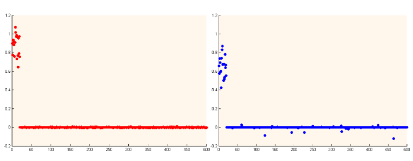
Figure 2: A typical result of the EWA (left panel) and the Lasso (right panel) in the setup of Example 1 with $n=200$, $M=500$ and $S=20$.

An interesting observation is that the EWA selects the set of nonzero coordinates of ${\boldsymbol{\lambda}}^{*}$ even better than the Lasso does. In fact, the approximate sparsity of the EWA is not very surprising, since in the noise-free linear models with orthogonal matrix $\mathbb{X}$, the symmetry of the prior implies that the EWA recovers the zero coordinates without error.

We note that the numerical results on the Lasso in Table 1 are substantially different from those reported in the short version of this paper published in the Proceeding of COLT 2009 [17]. This is because in [17] we used the R packages lars and glmnet, whereas here we use the MATLAB package l1_ls. It turns out that in the present example the latter provides more accurate approximation of the Lasso than the aforementioned R packages.

The running times of our algorithm are reasonable. For instance, in the case $n=m=100$ and $S=10$ the execution of our algorithm is only three times longer than the l1-ls implementation of the Lasso. On the other hand, the prediction error of our algorithm is more than twice smaller than that of the Lasso.

		$M=100$		$M=200$		$M=500$
	EWA	Lasso	EWA	Lasso	EWA	Lasso
$n=100$ $S=5$	0.063	0.344	0.064	0.385	0.087	0.453
	(0.039)	(0.132)	(0.043)	(0.151)	(0.054)	(0.161)
$n=100$ $S=10$	0.73725	1.680	1.153	1.918	1.891	2.413
	(0.699)	(0.621)	(1.091)	(0.677)	(1.522)	(0.843)
$n=100$ $S=15$	5.021	4.330	6.495	5.366	8.917	7.1828
	(1.593)	(1.262)	(1.794)	(1.643)	(2.186)	(2.069)
$n=200$ $S=5$	0.021	0.151	0.022	0.171	0.019	0.202
	(0.011)	(0.048)	(0.013)	(0.055)	(0.012)	(0.057)
$n=200$ $S=10$	0.106	0.658	0.108	0.753	0.117	0.887
	(0.047)	(0.169)	(0.048)	(0.198)	(0.051)	(0.239)
$n=200$ $S=20$	1.119	3.124	1.6015	3.734	2.728	4.502
	(0.696)	(0.806)	(1.098)	(0.907)	(1.791)	(1.063)

Table 1: Average loss $\|\widehat{\boldsymbol{\lambda}}-{\boldsymbol{\lambda}}^{*}\|^{2}$ of the estimators obtained by the EW-aggregate and the Lasso in Example 1. The standard deviation is given in parentheses.

5.2.2 Example 2

Consider model (1) where $Z_{i}$ are independent random variables uniformly distributed in the unit square $[0,1]^{2}$ and $\xi_{i}$ are iid ${\mathcal{N}}(0,\sigma^{2})$ random variables. For an integer $k>0$, we consider the indicator functions of rectangles with sides parallel to the axes and having as left-bottom vertex the origin and as right-top vertex a point of the form $(i/k,j/k)$, $(i,j)\in\mathbb{N}^{2}$. Formally, we define $\phi_{j}$ by

$$\phi_{(i-1)k+j}(x)={\rm 1}\mskip-4.5mu{\rm l}_{[0,i]\times[0,j]}(kx),\qquad\forall\,x\in[0,1]^{2}.$$

The underlying image $f$ we are trying to recover is taken as a superposition of a small number of rectangles of this form, that is $f(x)=\sum_{\ell=1}^{k^{2}}\lambda_{\ell}^{*}\phi_{\ell}(x)$, for all $x\in[0,1]^{2}$ with some ${{\boldsymbol{\lambda}}^{*}}$ having a small $\ell_{0}$-norm. We set $k=15$, $\|{{\boldsymbol{\lambda}}^{*}}\|_{0}=3$, $\lambda_{10}^{*}=\lambda_{100}^{*}=\lambda_{200}^{*}=1$. Thus, the cardinality of the dictionary is $M=k^{2}=225$.

In this example the functions $\phi_{j}$ are strongly correlated and therefore the assumptions like restricted isometry or low coherence are not fulfilled. Nevertheless, the Lasso succeeds in providing an accurate prediction (cf. Table 2). Furthermore, the Lasso with the theoretically justified choice of the regularization parameter $\sigma\sqrt{8\log M/n}$ is not much worse than the ideal Lasso-Gauss (LG) estimator. We call the LG estimator the ordinary least squares estimator in the reduced model where only the predictor variables selected at a preliminary Lasso step are kept. Of course, the performance of the LG procedure depends on the initial choice of the tuning parameter for the Lasso step. In our simulations, we use its ideal (oracle) value minimizing the prediction error and, therefore, we call the resulting procedure the ideal LG estimator.

	EWA	Lasso	Ideal LG
$\sigma=1,$ $n=100$	0.160	0.273	0.128
	(0.035)	(0.195)	(0.053)
$\sigma=2,$ $n=100$	0.210	0.759	0.330
	(0.072)	(0.562)	(0.145)
$\sigma=4,$ $n=100$	0.420	2.323	0.938
	(0.222)	(1.257)	(0.631)
$\sigma=1,$ $n=200$	0.130	0.187	0.069
	(0.030)	(0.124)	(0.031)
$\sigma=2,$ $n=200$	0.187	0.661	0.203
	(0.048)	(0.503)	(0.086)
$\sigma=4,$ $n=200$	0.278	2.230	0.571
	(0.132)	(1.137)	(0.324)

Table 2: Average loss $\int_{[0,1]^{2}}\big{(}\sum_{j}(\widehat{\lambda}_{j}-\lambda_{j}^{*})\phi_{j}(x)\big{)}^{2}\,dx$ of the the EWA, the Lasso and the ideal LG procedures in Example 2. The standard deviation is given in parentheses.

As expected, the EWA has a smaller predictive risk than the Lasso estimator. However, a surprising outcome of this experiment is the supremacy of the EWA over the ideal LG in the case of large noise variance. Of course, the LG procedure is faster. However, even from this point of view the EWA is rather attractive, since it takes less than two seconds to compute it in the present example.

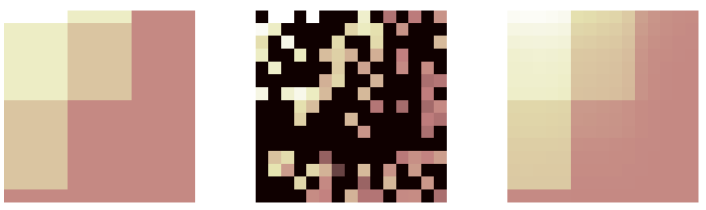
Figure 3: This figure shows a typical outcome in the setup of example 2 when $n=200$ and $k=15$. Left: the original image. Center: the observed noisy sample with $\sigma=0.5$. Pixels for which no observation is available are in black. Right: the image estimated by the EWA.

6 Conclusion and outlook

This paper contains two contributions: New oracle inequalities for EWA, and the LMC method for approximate computation of the EWA. The first oracle inequality presented in this work is in the line of the PAC-Bayesian bounds initiated by McAllester [30]. It is valid for any prior distribution and gives a bound on the risk of the EWA with an arbitrary family of functions. Next, we derive another inequality, which is adapted to the sparsity scenario and called the sparsity oracle inequality (SOI). In order to obtain it, we propose a prior distribution favoring sparse representations. The resulting EWA is shown to behave almost as well as the best possible linear combination within a residual term proportional to $M^{*}(\log M)/n$, where $M$ is the true dimension, $M^{*}$ is the number of atoms entering in the best linear combination and $n$ is the sample size. A remarkable fact is that this inequality is obtained under no condition on the relationship between different atoms.

Sparsity oracle inequalities similar to that of Theorem 2 are valid for the penalized empirical risk minimizers (ERM) with a $\ell_{0}$-penalty (proportional to the number of atoms involved in the representation). It is also well known that the problem of computing the $\ell_{0}$-penalized ERM is NP-hard. In contrast with this, we have shown that the numerical evaluation of the suggested EWA is a computationally tractable problem. We demonstrated that it can be efficiently solved by the LMC algorithm. Numerous simulations we did (some of which are included in this work) confirm our theoretical findings and, furthermore, suggest that the EWA is able to efficiently select the sparsity pattern. Theoretical justification of this fact, as well as more thorough investigation of the choice of parameters involved in the LMC algorithm, are interesting topics for future research.

Appendix: proofs of technical results

6.1 Proof of Proposition 2

For brevity, in this proof we denote by $\|\cdot\|$ the Euclidean norm in ${\mathbb{R}}^{M}$ and we set $\alpha=1$ in (10). The case of general $\alpha>0$ is treated analogously. Recall that for some small $h>0$ we have defined the $M$-dimensional Markov chain $({\boldsymbol{L}}^{E}_{k};k=0,1,2,\ldots)$ by (cf. (10) and (11)):

$${\boldsymbol{L}}^{E}_{k+1}={\boldsymbol{L}}^{E}_{k}+2h\beta^{-1}{\mathbb{X}}^{\top}({\mathbf{Y}}-{\mathbb{X}}{\boldsymbol{L}}^{E}_{k})-hg({\boldsymbol{L}}^{E}_{k})+\sqrt{2h}\,{\boldsymbol{\xi}}_{k+1},\quad{\boldsymbol{L}}^{E}_{0}=0,$$

where $({\boldsymbol{\xi}}_{k};k=1,2,\ldots)$ is a sequence of iid standard Gaussian vectors in ${\mathbb{R}}^{M}$, and

$$g:{\mathbb{R}}^{M}\to{\mathbb{R}}^{M}\quad\text{s.t.}\quad g({\boldsymbol{\lambda}})=\bigg{(}\frac{4\lambda_{1}}{\tau^{2}+\lambda_{1}^{2}}+\bar{\omega}^{\prime}(\lambda_{1}),\ldots,\frac{4\lambda_{M}}{\tau^{2}+\lambda_{M}^{2}}+\bar{\omega}^{\prime}(\lambda_{M})\bigg{)}^{\top}.$$

In what follows, we will use the fact that the function $g$ is bounded and satisfies ${\boldsymbol{\lambda}}^{\top}g({\boldsymbol{\lambda}})\geqslant 0$ for all ${\boldsymbol{\lambda}}\in{\mathbb{R}}^{M}$.

Let us prove some auxiliary results. Set ${\boldsymbol{v}}=2\beta^{-1}{\mathbb{X}}^{\top}{\mathbf{Y}}$, $\texttt{A}=2\beta^{-1}{\mathbb{X}}^{\top}{\mathbb{X}}$ and assume that $h\leqslant 1/\|\texttt{A}\|$. Without loss of generality we also assume that $T/h$ is an integer. In what follows, we denote by $C>0$ a constant whose value is not essential, does not depend neither on $T$ nor on $h$, and may vary from line to line. Since the function $g$ is bounded and ${\boldsymbol{\xi}}_{k+1}$ has zero mean, we have

$$\mathbf{E}[{\boldsymbol{L}}^{E}_{k+1}]=(I-h\texttt{A})\mathbf{E}[{\boldsymbol{L}}^{E}_{k}]+h\mathbf{E}[{\boldsymbol{v}}-g({\boldsymbol{L}}^{E}_{k})],\qquad\forall k\geqslant 0.$$

Therefore,

$$\|\mathbf{E}[{\boldsymbol{L}}^{E}_{k+1}]\|\leqslant\|(I-h\texttt{A})\mathbf{E}[{\boldsymbol{L}}^{E}_{k}]\|+Ch\leqslant\|\mathbf{E}[{\boldsymbol{L}}^{E}_{k}]\|+Ch,\qquad\forall k\geqslant 0.$$

By induction, we get

$$\|\mathbf{E}[{\boldsymbol{L}}^{E}_{k}]\|\leqslant Ckh\leqslant CT,\qquad\forall k\in[0,[T/h]].$$ (14)

Furthermore, since ${\boldsymbol{\xi}}_{k+1}$ is independent of ${\boldsymbol{L}}^{E}_{k}$ and $Y$, we have

$$\mathbf{E}[\|{\boldsymbol{L}}^{E}_{k+1}\|^{2}] = \mathbf{E}[\|{\boldsymbol{L}}^{E}_{k}+h{\boldsymbol{v}}-h\texttt{A}{\boldsymbol{L}}^{E}_{k}-hg({\boldsymbol{L}}^{E}_{k})\|^{2}]+2hM$$

$$\leqslant \mathbf{E}[\|{\boldsymbol{L}}^{E}_{k}\|^{2}+2h({\boldsymbol{L}}^{E}_{k})^{\top}({\boldsymbol{v}}-\texttt{A}{\boldsymbol{L}}^{E}_{k})-2h({\boldsymbol{L}}^{E}_{k})^{\top}g({\boldsymbol{L}}^{E}_{k})+h^{2}\|{\boldsymbol{v}}-\texttt{A}{\boldsymbol{L}}^{E}_{k}-g({\boldsymbol{L}}^{E}_{k})\|^{2}]+2hM$$

$$\leqslant \mathbf{E}[\|{\boldsymbol{L}}^{E}_{k}\|^{2}+2h({\boldsymbol{L}}^{E}_{k})^{\top}({\boldsymbol{v}}-\texttt{A}{\boldsymbol{L}}^{E}_{k})+2h^{2}\|\texttt{A}{\boldsymbol{L}}^{E}_{k}\|^{2}+2h^{2}\|{\boldsymbol{v}}-g({\boldsymbol{L}}^{E}_{k})\|^{2}]+2hM$$

$$\leqslant \mathbf{E}[\|{\boldsymbol{L}}^{E}_{k}\|^{2}+2h({\boldsymbol{L}}^{E}_{k})^{\top}{\boldsymbol{v}}-2h({\boldsymbol{L}}^{E}_{k})^{\top}(\texttt{A}-h\texttt{A}^{2}){\boldsymbol{L}}^{E}_{k}+2h^{2}\|{\boldsymbol{v}}-g({\boldsymbol{L}}^{E}_{k})\|^{2}]+2hM$$

$$\leqslant \mathbf{E}[\|{\boldsymbol{L}}^{E}_{k}\|^{2}]+2h\mathbf{E}[({\boldsymbol{L}}^{E}_{k})^{\top}]{\boldsymbol{v}}+Ch$$

$$\leqslant \mathbf{E}[\|{\boldsymbol{L}}^{E}_{k}\|^{2}]+ChT,\qquad\forall k\in[0,[T/h]].$$

Once again, using induction, we get

$$\mathbf{E}[\|{\boldsymbol{L}}^{E}_{k}\|^{2}]\leqslant CkhT\leqslant CT^{2},\qquad\forall k\in[0,[T/h]].$$ (15)

This implies, in particular, that $(h/T)\mathbf{E}[\|{\boldsymbol{L}}^{E}_{[T/h]}\|^{2}]\to 0$ as $h\to 0$ for any fixed $T$.

Proof of Step 1

Denote by $\psi$ the function

$$\psi({\boldsymbol{\lambda}})={\boldsymbol{v}}-\texttt{A}{\boldsymbol{\lambda}}-g({\boldsymbol{\lambda}}),\qquad\forall{\boldsymbol{\lambda}}\in{\mathbb{R}}^{M},$$

and define the continuous-time random process $(\tilde{\boldsymbol{L}}_{t,h};0\leqslant t\leqslant[T/h]h)$ by

$$d\tilde{\boldsymbol{L}}_{t,h}=\sum_{k=0}^{[T/h]-1}\psi({\boldsymbol{L}}^{E}_{k}){\rm 1}\mskip-4.5mu{\rm l}_{[kh,(k+1)h)}(t)\,dt+\sqrt{2}d{\boldsymbol{W}}_{t},\quad\tilde{\boldsymbol{L}}_{0,h}=\boldsymbol{0},$$ (16)

where ${\boldsymbol{W}}_{t}$ is a $M$-dimensional Brownian motion satisfying ${\boldsymbol{W}}_{kh}={\boldsymbol{\xi}}_{k}$, for all $k$. The rigorous construction of ${\boldsymbol{W}}$ can be done as follows. Let $({\boldsymbol{B}}_{t};0\leqslant t\leqslant T)$ be a $M$-dimensional Brownian motion defined on the same probability space as the sequence $({\boldsymbol{\xi}}_{k};0\leqslant k\leqslant[T/h])$ and independent of $({\boldsymbol{\xi}}_{k};0\leqslant k\leqslant[T/h])$. One can check that the process defined by

$${\boldsymbol{W}}_{t}={\boldsymbol{\xi}}_{k}+{\boldsymbol{B}}_{t}-{\boldsymbol{B}}_{kh}-\Big{(}\frac{t}{h}-k\Big{)}\big{(}{\boldsymbol{B}}_{(k+1)h}-{\boldsymbol{B}}_{kh}-{\boldsymbol{\xi}}_{k+1}\big{)},\qquad t\in[kh,(k+1)h[$$

is a Brownian motion and satisfies ${\boldsymbol{W}}_{kh}={\boldsymbol{\xi}}_{k}$.

By the Cauchy-Schwarz inequality,

$$\mathbf{E}\bigg{[}\bigg{\|}\frac{h}{T}\sum_{k=0}^{[T/h]-1}{\boldsymbol{L}}^{E}_{k}-\frac{1}{T}\int_{0}^{T}\tilde{\boldsymbol{L}}_{t,h}\,dt\bigg{\|}^{2}\bigg{]} = \mathbf{E}\bigg{[}\bigg{\|}\frac{1}{T}\int_{0}^{T}\big{(}\sum_{k=0}^{[T/h]-1}\tilde{\boldsymbol{L}}_{kh,h}{\rm 1}\mskip-4.5mu{\rm l}_{[kh,(k+1)h)}(t)-\tilde{\boldsymbol{L}}_{t,h}\big{)}\,dt\bigg{\|}^{2}\bigg{]}$$

$$\leqslant \frac{1}{T}\sum_{k=0}^{[T/h]-1}\int_{kh}^{(k+1)h}\mathbf{E}\big{[}\|\tilde{\boldsymbol{L}}_{t,h}-\tilde{\boldsymbol{L}}_{kh,h}\|^{2}\big{]}\,dt$$

$$\leqslant \frac{2}{T}\sum_{k=0}^{[T/h]-1}\int_{kh}^{(k+1)h}\limits\mathbf{E}\big{[}h^{2}\|\psi({\boldsymbol{L}}^{E}_{k})\|^{2}+2\|{\boldsymbol{W}}_{t}-{\boldsymbol{W}}_{kh}\|^{2}\big{]}\,dt$$

$$\leqslant \frac{2h^{3}}{T}\sum_{k=0}^{[T/h]-1}\mathbf{E}\big{[}\|\psi({\boldsymbol{L}}^{E}_{k})\|^{2}\big{]}+4Mh.$$

Using the inequality $\|\psi({\boldsymbol{\lambda}})\|\leqslant C(1+\|{\boldsymbol{\lambda}}\|)$ and (15), we get

$$\mathbf{E}\bigg{[}\bigg{\|}\frac{h}{T}\sum_{k=0}^{[T/h]-1}{\boldsymbol{L}}^{E}_{k}-\frac{1}{T}\int_{0}^{T}\tilde{\boldsymbol{L}}_{t,h}\,dt\bigg{\|}^{2}\bigg{]} \leqslant Ch^{2}+\frac{Ch^{3}}{T}\sum_{k=0}^{[T/h]-1}\mathbf{E}\big{[}\|{\boldsymbol{L}}^{E}_{k}\|^{2}\big{]}+4Mh$$

$$\leqslant Ch(1+hT^{2}).$$

This completes the proof of the Step 1.

Proof of Step 2

Using (15) we obtain

$$\mathbf{E}[\|\textsf{T}_{2}\|] \leqslant \frac{1}{T}\int_{0}^{T}\mathbf{E}[\|\tilde{\boldsymbol{L}}_{t,h}\|{\rm 1}\mskip-4.5mu{\rm l}_{[A,+\infty]}(\|\tilde{\boldsymbol{L}}_{t,h}\|)]\leqslant\frac{1}{TA}\int_{0}^{T}\mathbf{E}[\|\tilde{\boldsymbol{L}}_{t,h}\|^{2}]\,dt$$ (17)

$$\leqslant \frac{C}{TA}\sum_{k=0}^{[T/h]-1}\int_{kh}^{(k+1)h}\big{(}\mathbf{E}[\|{\boldsymbol{L}}^{E}_{k}\|^{2}]+h^{2}\mathbf{E}[\|\psi({\boldsymbol{L}}^{E}_{k})+\texttt{A}{\boldsymbol{L}}^{E}_{k}\|^{2}]+\mathbf{E}[\|{\boldsymbol{W}}_{t}-{\boldsymbol{W}}_{kh}\|^{2}]\big{)}\,dt$$

$$\leqslant \frac{C}{TA}\sum_{k=0}^{[T/h-1]}h\big{(}\mathbf{E}[\|{\boldsymbol{L}}^{E}_{k}\|^{2}]+Ch^{2}+Mh\big{)}\leqslant\frac{CT^{2}}{A}.$$

Thus, choosing, for example, $A=T^{3}$ we guarantee that $\lim_{T\to\infty}\varlimsup_{h\to 0}\mathbf{E}[\|\textsf{T}_{2}\|]=0$.

Proof of Step 3

First, note that (16) can be written in the form

$$d\tilde{\boldsymbol{L}}_{t,h}=\tilde{\psi}(\tilde{\boldsymbol{L}}_{h},t)\,dt+\sqrt{2}d{\boldsymbol{W}}_{t},\quad\tilde{\boldsymbol{L}}_{0,h}=\boldsymbol{0},$$

where $\tilde{\psi}(\tilde{\boldsymbol{L}}_{h},t)$ is a non-anticipative process that equals $\psi(\tilde{\boldsymbol{L}}_{kh,h})$ when $t\in[kh,(k+1)h)$. Recall that the Langevin diffusion is defined by the stochastic differential equation

$$d{\boldsymbol{L}}_{t}=\psi({\boldsymbol{L}}_{t})\,dt+\sqrt{2}d{\boldsymbol{W}}_{t},\quad{\boldsymbol{L}}_{0}=\boldsymbol{0}.$$

Therefore, the probability distributions ${\mathbf{P}}_{{\boldsymbol{L}},T}$ and ${\mathbf{P}}_{\tilde{\boldsymbol{L}}_{h},T}$ induced by, respectively, $({\boldsymbol{L}}_{t};0\leqslant t\leqslant T)$ and $(\tilde{\boldsymbol{L}}_{t,h};0\leqslant t\leqslant T)$ are mutually absolutely continuous and the corresponding Radon-Nykodim derivatives are given by Girsanov formula:

$$\frac{d{\mathbf{P}}_{\tilde{\boldsymbol{L}}_{h},T}}{d{\mathbf{P}}_{{\boldsymbol{L}},T}}({\boldsymbol{L}})=\exp\Big{\{}\frac{1}{\sqrt{2}}\int_{0}^{T}(\tilde{\psi}({\boldsymbol{L}},t)-\psi({\boldsymbol{L}}_{t}))^{\top}\big{(}d{\boldsymbol{L}}_{t}-\psi({\boldsymbol{L}}_{t})\,dt\big{)}-\frac{1}{4}\int_{0}^{T}\|\tilde{\psi}({\boldsymbol{L}},t)-\psi({\boldsymbol{L}}_{t})\|^{2}\,dt\Big{\}}.$$

This implies that the Kullback-Leibler divergence between ${\mathbf{P}}_{\tilde{\boldsymbol{L}}_{h},T}$ and ${\mathbf{P}}_{{\boldsymbol{L}},T}$ is given by

$$\mathcal{K}\big{(}{\mathbf{P}}_{{\boldsymbol{L}},T}|\!|{\mathbf{P}}_{\tilde{\boldsymbol{L}}_{h},T}\big{)}=-\mathbf{E}\Big{[}\log\Big{(}\frac{d{\mathbf{P}}_{\tilde{\boldsymbol{L}}_{h},T}}{d{\mathbf{P}}_{{\boldsymbol{L}},T}}({\boldsymbol{L}})\Big{)}\Big{]}=\frac{1}{4}\int_{0}^{T}\mathbf{E}\big{[}\|\tilde{\psi}({\boldsymbol{L}},t)-\psi({\boldsymbol{L}}_{t})\|^{2}\big{]}\,dt.$$

Using the expressions of $\psi$ and $\tilde{\psi}$, as well as the fact that the function $\psi$ is Lipschitz continuous, we can bound the divergence above as follows:

$$\mathcal{K}\big{(}{\mathbf{P}}_{{\boldsymbol{L}},T}|\!|{\mathbf{P}}_{\tilde{\boldsymbol{L}}_{h},T}\big{)} = \frac{1}{4}\sum_{k=0}^{[T/h]-1}\int_{kh}^{(k+1)h}\mathbf{E}\big{[}\|\psi({\boldsymbol{L}}_{kh})-\psi({\boldsymbol{L}}_{t})\|^{2}\big{]}\,dt$$

$$\leqslant C\sum_{k=0}^{[T/h]-1}\int_{kh}^{(k+1)h}\mathbf{E}\big{[}\|{\boldsymbol{L}}_{kh}-{\boldsymbol{L}}_{t}\|^{2}\big{]}\,dt$$

$$= C\sum_{k=0}^{[T/h]-1}\int_{kh}^{(k+1)h}\mathbf{E}\Big{[}\Big{\|}\int_{kh}^{t}\psi({\boldsymbol{L}}_{s})\,ds+\sqrt{2}({\boldsymbol{W}}_{t}-{\boldsymbol{W}}_{kh})\Big{\|}^{2}\Big{]}\,dt.$$

From the Cauchy-Schwarz inequality and the fact that $\|\psi({\boldsymbol{\lambda}})\|\leqslant C(1+\|{\boldsymbol{\lambda}}\|)$ we obtain

$$\mathcal{K}\big{(}{\mathbf{P}}_{{\boldsymbol{L}},T}|\!|{\mathbf{P}}_{\tilde{\boldsymbol{L}}_{h},T}\big{)} \leqslant C\sum_{k=0}^{[T/h]-1}\int_{kh}^{(k+1)h}h\int_{kh}^{t}\mathbf{E}\big{[}\|\psi({\boldsymbol{L}}_{s})\|^{2}\big{]}\,ds\,dt+ChT$$

$$\leqslant Ch^{2}\sum_{k=0}^{[T/h]-1}\int_{kh}^{(k+1)h}\mathbf{E}\big{[}\|\psi({\boldsymbol{L}}_{s})\|^{2}\big{]}\,ds+ChT$$

$$\leqslant Ch^{2}\int_{0}^{T}\mathbf{E}\big{[}\|\psi({\boldsymbol{L}}_{s})\|^{2}\big{]}\,ds+ChT$$

$$\leqslant Ch^{2}\int_{0}^{T}\mathbf{E}\big{[}\|{\boldsymbol{L}}_{s}\|^{2}\big{]}\,ds+ChT.$$

Since by Proposition 1 the expectation of $\|{\boldsymbol{L}}_{s}\|^{2}$ is bounded uniformly in $s$, we get $\mathcal{K}\big{(}{\mathbf{P}}_{{\boldsymbol{L}},T}|\!|{\mathbf{P}}_{\tilde{\boldsymbol{L}}_{h},T}\big{)}\to 0$ as $h\to 0$. In view of Pinsker’s inequality, cf, e.g., [38], this implies that the distribution ${\mathbf{P}}_{\tilde{\boldsymbol{L}}_{h},T}$ converges to ${\mathbf{P}}_{{\boldsymbol{L}},T}$ in total variation as $h\to 0$. Thus, (13) follows.

Proof of Step 4

To prove that the right hand side of (13) tends to zero as $T\to+\infty$, we use the fact that the process ${\boldsymbol{L}}_{t}$ has the geometrical mixing property with $D({\boldsymbol{\lambda}})=e^{\alpha\|{\boldsymbol{\lambda}}\|_{2}}$. Bias-variance decomposition yields:

$$\mathbf{E}\bigg{[}\bigg{(}\frac{1}{T}\int_{0}^{T}\!\!G({\boldsymbol{L}}_{t})\,dt-\int G({\boldsymbol{\lambda}})p_{V}({\boldsymbol{\lambda}})d{\boldsymbol{\lambda}}\bigg{)}^{2}\bigg{]}=\frac{1}{T^{2}}\textbf{Var}\Big{[}\int_{0}^{T}\!\!G({\boldsymbol{L}}_{t})\,dt\Big{]}+\bigg{(}\frac{1}{T}\int_{0}^{T}\mathbf{E}_{0}[G({\boldsymbol{L}}_{t})]\,dt-\int G({\boldsymbol{\lambda}})p_{V}({\boldsymbol{\lambda}})d{\boldsymbol{\lambda}}\bigg{)}^{2}\!\!.$$

The second term on the right hand side of the last display tends to zero as $T\to\infty$ in view of Proposition 1, while the first term can be evaluated as follows:

$$\frac{1}{T^{2}}\textbf{Var}\Big{[}\int_{0}^{T}G({\boldsymbol{L}}_{t})\,dt\Big{]} = \frac{1}{T^{2}}\int_{0}^{T}\int_{0}^{T}\textbf{Cov}_{0}\big{[}G({\boldsymbol{L}}_{t}),G({\boldsymbol{L}}_{s})\big{]}\,dt\,ds$$

$$\leqslant \frac{C}{T^{2}}\int_{0}^{T}\int_{0}^{T}\rho_{V}^{-|t-s|}\,dt\,ds\leqslant CT^{-1}.$$

This completes the proof of Proposition 2.

6.2 Proof of Lemma 3

We first prove a simple auxiliary result, cf. Lemma 4 below. Then, the two claims of Lemma 3 are proved in Lemmas 5 and 6, respectively.

Lemma 4.

For every $M\in\mathbb{N}$ and every $s>M$, the following inequality holds:

$$\frac{1}{(\pi/2)^{M}}\int_{\big{\{}u:\|u\|_{1}>s\big{\}}}\prod_{j=1}^{M}\frac{du_{j}}{(1+u_{j}^{2})^{2}}\leqslant\frac{M}{(s-M)^{2}}.$$

Proof.

Let $U_{1},\ldots,U_{M}$ be iid random variables drawn from the scaled Student $t(3)$ distribution having as density the function $u\mapsto 2/\big{[}\pi(1+u^{2})^{2}\big{]}$. One easily checks that $\mathbf{E}[U_{1}^{2}]=1$. Furthermore, with this notation, we have

$$\frac{1}{(\pi/2)^{M}}\int_{\big{\{}u:\|u\|_{1}>s\big{\}}}\prod_{j=1}^{M}\frac{du_{j}}{(1+u_{j}^{2})^{2}}={\mathbf{P}}\Big{(}\sum_{j=1}^{M}|U_{j}|\geqslant s\Big{)}.$$

In view of Chebyshev’s inequality the last probability can be bounded as follows:

$${\mathbf{P}}\Big{(}\sum_{j=1}^{M}|U_{j}|\geqslant s\Big{)}\leqslant\frac{M\mathbf{E}[U_{1}^{2}]}{(s-M\mathbf{E}[|U_{1}|])^{2}}\leqslant\frac{M}{(s-M)^{2}}$$

and the desired inequality follows. ∎

Lemma 5.

Let the assumptions of Theorem 2 be satisfied and let $p_{0}$ be the probability measure defined by (5). If $M\geqslant 2$ then

$$\int_{\Lambda}(\lambda_{1}-\lambda_{1}^{*})^{2}p_{0}(d{\boldsymbol{\lambda}})\leqslant 4\tau^{2}e^{4M\alpha\tau}.$$

Proof.

Using the change of variables $u=({\boldsymbol{\lambda}}-{{\boldsymbol{\lambda}}^{*}})/\tau$ we write

$$\int_{\Lambda}(\lambda_{1}-\lambda_{1}^{*})^{2}p_{0}(d{\boldsymbol{\lambda}})=C_{M}\tau^{2}\int_{B_{1}(2M)}u_{1}^{2}\Big{(}\prod_{j=1}^{M}(1+u_{j}^{2})^{-2}e^{-\bar{\omega}(\alpha\tau u_{j})}\Big{)}\,du$$

with

$$C_{M}=\Big{(}\int_{B_{1}(2M)}\Big{(}\prod_{j=1}^{M}(1+u_{j}^{2})^{-2}e^{-\bar{\omega}(\tau\alpha u_{j})}\Big{)}\,du\Big{)}^{-1}$$ (18)

where $u_{j}$ are the components of $u$. Bounding the functions $e^{-\bar{\omega}(\tau\alpha u_{j})}$ by one, extending the integration from $B_{1}(2M)$ to ${\mathbb{R}}^{M}$ and using the inequality $\int_{\mathbb{R}}u_{1}^{2}(1+u_{1}^{2})^{-2}du_{1}\leqslant\pi$, we get

$$\int_{\Lambda}(\lambda_{1}-\lambda_{1}^{*})^{2}p_{0}(d{\boldsymbol{\lambda}})\leqslant C_{M}\tau^{2}\pi\Big{(}\int_{{\mathbb{R}}}(1+t^{2})^{-2}\,dt\Big{)}^{M-1}=2C_{M}\tau^{2}(\pi/2)^{M},$$

where we used that the primitive of the function $(1+x^{2})^{-2}$ is $\frac{1}{2}\arctan(x)+\frac{x}{2(1+x^{2})}$. To bound $C_{M}$ we first use the inequality $\bar{\omega}(x)\leqslant 2|x|$ which yields:

$$C_{M}\leqslant\Big{(}\int_{B_{1}(2M)}e^{-2\alpha\tau\|u\|_{1}}\,\prod_{j=1}^{M}\frac{du_{j}}{(1+u_{j}^{2})^{2}}\Big{)}^{-1}\\ \leqslant e^{4\alpha\tau M}\Big{(}\int_{B_{1}(2M)}\prod_{j=1}^{M}\frac{du_{j}}{(1+u_{j}^{2})^{2}}\Big{)}^{-1}.$$ (19)

In view of (19) and Lemma 3 we have

$$C_{M}\leqslant e^{4\alpha\tau M}(2/\pi)^{M}\big{(}1-1/M\big{)}^{-1}\leqslant 2e^{4\alpha\tau M}(2/\pi)^{M}$$ (20)

for $M\geqslant 2$. Combining these estimates we get

$$\int_{\Lambda}(\lambda_{1}-\lambda_{1}^{*})^{2}p_{0}(d{\boldsymbol{\lambda}})\leqslant 4\tau^{2}e^{4\alpha\tau M}$$

and the desired inequality follows. ∎

Lemma 6.

Let the assumptions of Theorem 2 be satisfied and let $p_{0}$ be the probability measure defined by (5). Then

$$\mathcal{K}(p_{0},\pi)\leqslant 2\Big{(}\alpha\|{{\boldsymbol{\lambda}}^{*}}\|_{1}+\sum_{j=1}^{M}2\log(1+|\lambda_{\!j}^{*}|/\tau)\Big{)}+(1+4M\alpha\tau).$$

Proof.

The definition of $\pi$, $p_{0}$ and of the Kullback-Leibler divergence imply that

$$\mathcal{K}(p_{0},\pi) =\int_{B_{1}(2M\tau)}\log\Bigg{\{}C_{M}C_{\alpha,\tau,R}\prod_{j=1}^{M}\frac{(\tau^{2}+\lambda_{\!j}^{2})^{2}e^{\bar{\omega}(\alpha\lambda_{\!j})}}{(\tau^{2}+(\lambda_{\!j}-\lambda_{\!j}^{*})^{2})^{2}e^{\bar{\omega}(\alpha(\lambda_{\!j}-\lambda_{\!j}^{*}))}}\Bigg{\}}p_{0}(d{\boldsymbol{\lambda}})$$ (21)

$$=\log(C_{M}C_{\alpha,\tau,R})+2\sum_{j=1}^{M}\int_{B_{1}(2M\tau)}\log\Bigg{\{}\frac{\tau^{2}+\lambda_{\!j}^{2}}{\tau^{2}+(\lambda_{\!j}-\lambda_{\!j}^{*})^{2}}\Bigg{\}}p_{0}(d{\boldsymbol{\lambda}})$$

$$\qquad+\sum_{j=1}^{M}\int_{B_{1}(2M\tau)}\big{(}\bar{\omega}(\alpha\lambda_{\!j})-\bar{\omega}(\alpha(\lambda_{\!j}-\lambda_{\!j}^{*}))\big{)}p_{0}(d{\boldsymbol{\lambda}}).$$

We now successively evaluate the three terms on the RHS of (21). First, in view of (4), we have

$$C_{\alpha,\tau,R}=\int_{B_{1}(R)}\prod_{j=1}^{M}\frac{e^{-\bar{\omega}(\alpha u_{j}\tau)}}{(1+u_{j}^{2})^{2}}\,du_{j}\leqslant\Big{(}\int_{\mathbb{R}}(1+u_{j}^{2})^{-2}\,du_{j}\Big{)}^{M}=(\pi/2)^{M}.$$

This and (20) imply $\log(C_{M}C_{\alpha,\tau,R})\leqslant 1+4M\alpha\tau$.

To evaluate the second term on the RHS of (21) we use that

$$\frac{\tau^{2}+\lambda^{2}_{j}}{\tau^{2}+(\lambda_{\!j}-\lambda_{\!j}^{*})^{2}} = 1+\frac{2\tau(\lambda_{\!j}-\lambda_{\!j}^{*})}{\tau^{2}+(\lambda_{\!j}-\lambda_{\!j}^{*})^{2}}(\lambda_{\!j}^{*}/\tau)+\frac{{\lambda_{\!j}^{*}}^{2}}{\tau^{2}+(\lambda_{\!j}-\lambda_{\!j}^{*})^{2}}$$

$$\leqslant 1+|\lambda_{\!j}^{*}/\tau|+(\lambda_{\!j}^{*}/\tau)^{2}\leqslant(1+|\lambda_{\!j}^{*}/\tau|)^{2}.$$

This entails that the second term on the RHS of (21) is bounded from above by $\sum_{j=1}^{M}2\log(1+|\lambda_{\!j}^{*}|/\tau)$. Finally, since the derivative of $\bar{\omega}(\cdot)$ is bounded in absolute value by $2$, we have $\bar{\omega}(\alpha\lambda_{\!j})-\bar{\omega}(\alpha(\lambda_{\!j}-\lambda_{\!j}^{*}))\leqslant 2\alpha|\lambda_{\!j}^{*}|$ which implies:

$$\sum_{j=1}^{M}\int_{B_{1}(2M\tau)}\big{(}\bar{\omega}(\alpha\lambda_{\!j})-\bar{\omega}\big{(}\alpha(\lambda_{\!j}-\lambda_{\!j}^{*})\big{)}\big{)}p_{0}(d{\boldsymbol{\lambda}})\leqslant 2\alpha\|{{\boldsymbol{\lambda}}^{*}}\|_{1}.$$

Combining these inequalities we get the lemma. ∎

6.3 Proofs of remarks 1-6

We only prove Remarks 2 and 6, since the proofs of the remaining remarks are straghtforward.

6.3.1 Proof of Remark 2

Let $\xi$ be a random variable satisfying ${\mathbf{P}}(\xi=\pm\sigma)=1/2$ and let $U$ be another random variable, independent of $\xi$ and drawn from the uniform distribution on $[-1,1]$. Recall that $\zeta=(1+\gamma)\sigma\mathop{\rm sgn}[\sigma^{-1}\xi-(1+\gamma)U]-\xi$.

We start by proving that $\xi+\zeta$ has the same distribution as $(1+\gamma)\xi$. Clearly, $|\xi+\zeta|$ equals $(1+\gamma)\sigma$ almost surely. Furthermore,

$${\mathbf{P}}\big{(}\xi+\zeta=(1+\gamma)\sigma\big{)}\!\!\!\!\! = \!\!\!\!{\mathbf{P}}\big{(}\sigma^{-1}\xi\geqslant(1+\gamma)U\big{)}$$

$$= \!\!\!\!\frac{1}{2}\Big{(}{\mathbf{P}}\big{(}1\geqslant(1+\gamma)U\big{)}+{\mathbf{P}}\big{(}-1\geqslant(1+\gamma)U\big{)}\Big{)}$$

$$= \!\!\!\!\frac{1}{4}\Bigg{(}\Big{(}\frac{1}{1+\gamma}+1\Big{)}+\Big{(}-\frac{1}{1+\gamma}+1\Big{)}\Bigg{)}=\frac{1}{2}.$$

This entails that ${\mathbf{P}}\big{(}\xi+\zeta=-(1+\gamma)\sigma\big{)}=1/2$ and, therefore, the distributions of $\xi+\zeta$ and $(1+\gamma)\xi$ coincide.

We compute now the conditional expectation $\mathbf{E}[\zeta|\xi]$. Since $U$ and $\xi$ are independent, we have

$$\mathbf{E}[\zeta\,|\,\xi=\sigma]\!\!\!\!\! = \!\!\!\!(1+\gamma)\sigma\mathbf{E}\big{(}\mathop{\rm sgn}[1-(1+\gamma)U]\big{)}-\sigma=0.$$

Similarly, $\mathbf{E}[\zeta\,|\,\xi=-\sigma]=0$.

To complete the proof of Remark 2, it remains to show that part iii) of Assumption N is fulfilled. Indeed,

$$\frac{\log\mathbf{E}[e^{t\zeta}\,|\,\xi=\sigma]}{t^{2}\gamma\sigma^{2}}\!\!\!\!\! = \!\!\!\!\frac{1}{t^{2}\gamma\sigma^{2}}\log\Bigg{(}e^{t\gamma\sigma}\frac{2+\gamma}{2(1+\gamma)}+e^{-t(2+\gamma)\sigma}\frac{\gamma}{2(1+\gamma)}\Bigg{)}$$

$$= \!\!\!\!\frac{1}{t^{2}\gamma\sigma^{2}}\Bigg{[}t\gamma\sigma+\log\Bigg{(}1+\Bigg{\{}e^{-2t(1+\gamma)\sigma}-1\Bigg{\}}\frac{\gamma}{2(1+\gamma)}\Bigg{)}\Bigg{]}.$$

Applying the inequality of [16, Lemma 3] with $\alpha_{0}=2(1+\gamma)/\gamma$ and $x=t\gamma\sigma$, we get

$$\frac{\log\mathbf{E}[e^{t\zeta}\,|\,\xi=\sigma]}{t^{2}\gamma\sigma^{2}}\!\!\!\! \leqslant \!\!\!\!\frac{1}{t^{2}\gamma\sigma^{2}}(t\gamma\sigma)^{2}\frac{(1+\gamma)}{\gamma}=1+\gamma$$

and the desired result follows.

6.3.2 Proof of Remark 6

We start by computing the conditional moment generating function (Laplace transform) of $\zeta$ given $\xi$:

$$\mathbf{E}\big{[}e^{t\zeta}\,\big{|}\,\xi=a\big{]}\!\!\!\!\! = \!\!\!\!e^{-ta}\mathbf{E}\big{[}e^{t(\zeta+\xi)}\,\big{|}\,\xi=a\big{]}$$ (22)

$$= \!\!\!\!e^{-ta}\Bigg{(}e^{t(1+\gamma)|a|}{\mathbf{P}}\big{(}\mathop{\rm sgn}(a)>(1+\gamma)U\big{)}+e^{-t(1+\gamma)|a|}{\mathbf{P}}\big{(}\mathop{\rm sgn}(a)<(1+\gamma)U\big{)}\Bigg{)}$$

$$= \!\!\!\!e^{-ta}\Bigg{(}e^{t(1+\gamma)a}\frac{2+\gamma}{2+2\gamma}+e^{-t(1+\gamma)a}\frac{\gamma}{2+2\gamma}\Bigg{)}.$$

Using (22) we obtain

$$\mathbf{E}\big{[}e^{t(\zeta+\xi)}\big{]}\!\!\!\!\! = \!\!\!\!\mathbf{E}\Big{[}\mathbf{E}\big{[}e^{t(\zeta+\xi)}\,\big{|}\,\xi\big{]}\Big{]}=\frac{2+\gamma}{2+2\gamma}\mathbf{E}\big{[}e^{-t(1+\gamma)\xi}\big{]}+\frac{\gamma}{2+2\gamma}\mathbf{E}\big{[}e^{t(1+\gamma)\xi}\big{]}=\mathbf{E}\big{[}e^{t(1+\gamma)\xi}\big{]},$$

since the symmetry of $\xi$ implies that $\mathbf{E}\big{[}e^{-t(1+\gamma)\xi}\big{]}=\mathbf{E}\big{[}e^{t(1+\gamma)\xi}\big{]}$ for every $t$. Thus, $\zeta+\xi$ has the same distribution as $(1+\gamma)\xi$.

On the other hand, taking the derivatives of both sides of (22) and using the fact that $\mathbf{E}[\zeta\,|\,\xi=a]$ equals to the derivative of the moment generating function $\mathbf{E}[e^{t\zeta}\,|\,\xi=a]$ at $t=0$, we obtain that $\mathbf{E}[\zeta\,|\,\xi=a]=0$ for every $a\in[-B,B]$. To complete the proof of Remark 6 we apply [16, Lemma 3] to the right hand side of (22). This yields

$$\log\Big{(}\mathbf{E}\big{[}e^{t\zeta}\,\big{|}\,\xi=a\big{]}\Big{)}\!\!\!\! \leqslant \!\!\!\!(t\gamma a)^{2}\frac{1+\gamma}{\gamma}\leqslant(tB)^{2}\gamma(1+\gamma).$$

Therefore, part iii) of Assumption N is satisfied with $v(a)\leqslant B^{2}$. This completes the proof of Remark 6.

References

References

- Abramovich et al. [2007] Abramovich, F., Grinshtein, V., Pensky, M., 2007. On optimality of Bayesian testimation in the normal means problem. Ann. Statist. 35, 2261–2286.
- Alquier [2008] Alquier, P., 2008. Pac-Bayesian bounds for randomized empirical risk minimizers. Math. Methods Statist. 17 (4), 1–26.
- Audibert [2009] Audibert, J.-Y., 2009. Fast learning rates in statistical inference through aggregation. Ann. Statist. 37 (4), 1591–1646.
- Bickel et al. [2009] Bickel, P. J., Ritov, Y., Tsybakov, A. B., 2009. Simultaneous analysis of lasso and Dantzig selector. Ann. Statist. 37 (4), 1705–1732.
- Bunea et al. [2007a] Bunea, F., Tsybakov, A., Wegkamp, M., 2007a. Sparsity oracle inequalities for the Lasso. Electronic J. of Statist. 1, 169–194.
- Bunea et al. [2006] Bunea, F., Tsybakov, A. B., Wegkamp, M., 2006. Aggregation and sparsity via penalized least squares. In: Learning theory. Vol. 4005 of Lecture Notes in Comput. Sci. Springer, Berlin, pp. 379–391.
- Bunea et al. [2007b] Bunea, F., Tsybakov, A. B., Wegkamp, M., 2007b. Aggregation for Gaussian regression. Ann. Statist. 35 (4), 1674–1697.
- Candès and Tao [2006] Candès, E., Tao, T., 2006. Near-optimal signal recovery from random projections: universal encoding strategies? IEEE Trans. Inform. Theory 52 (12), 5406–5425.
- Candès and Tao [2007] Candès, E., Tao, T., 2007. The Dantzig selector: statistical estimation when is much larger than . Ann. Statist. 35 (6), 2313–2351.
- Catoni [2004] Catoni, O., 2004. Statistical learning theory and stochastic optimization. Lecture Notes in Mathematics. Springer-Verlag, Berlin.
- Catoni [2007] Catoni, O., 2007. Pac-Bayesian Supervised Classification: The Thermodynamics of Statistical Learning. Vol. 56. IMS Lecture Notes Monograph Series.
- Cesa-Bianchi et al. [2004] Cesa-Bianchi, N., Conconi, A., Gentile, C., 2004. On the generalization ability of on-line learning algorithms. IEEE Trans. Inform. Theory 50 (9), 2050–2057.
- Cesa-Bianchi et al. [1997] Cesa-Bianchi, N., Freund, Y., Haussler, D., Helmbold, D. P., Schapire, R. E., Warmuth, M. K., 1997. How to use expert advice. J. ACM 44 (3), 427–485.
- Cesa-Bianchi and Lugosi [2006] Cesa-Bianchi, N., Lugosi, G., 2006. Prediction, learning, and games. Cambridge University Press, Cambridge.
- Dalalyan and Tsybakov [2007] Dalalyan, A. S., Tsybakov, A. B., 2007. Aggregation by exponential weighting and sharp oracle inequalities. In: Learning theory. Vol. 4539 of Lecture Notes in Comput. Sci. Springer, Berlin, pp. 97–111.
- Dalalyan and Tsybakov [2008] Dalalyan, A. S., Tsybakov, A. B., 2008. Aggregation by exponential weighting, sharp PAC-Bayesian bounds and sparsity. Mach. Learn. 72 (1-2), 39–61.
- Dalalyan and Tsybakov [2009] Dalalyan, A. S., Tsybakov, A. B., 2009. Sparse regression learning by aggregation and Langevin Monte-Carlo. In: COLT-2009.
- Donoho et al. [2006] Donoho, D., Elad, M., Temlyakov, V., 2006. Stable recovery of sparse overcomplete representations in the presence of noise. IEEE Trans. Inform. Theory 52 (1), 6–18.
- Efron et al. [2004] Efron, B., Hastie, T., Johnstone, I., Tibshirani, R., 2004. Least angle regression. Ann. Statist. 32 (2), 407–499.
- Gaïffas and Lecué [2007] Gaïffas, S., Lecué, G., 2007. Optimal rates and adaptation in the single-index model using aggregation. Electron. J. Stat. 1, 538–573.
- Giraud et al. [2009] Giraud, C., Huet, S., Verzelen, N., 2009. Graph selection with GGMselect. preprint, available on arXiv:0907.0619v1.
- Haussler et al. [1998] Haussler, D., Kivinen, J., Warmuth, M., 1998. Sequential prediction of individual sequences under general loss functions. IEEE Trans. Inform. Theory 44 (5), 1906–1925.
- Johnstone and Silverman [2005] Johnstone, I., Silverman, B., 2005. Empirical Bayes selection of wavelet thresholds. Ann. Statist 33, 1700–1752.
- Juditsky et al. [2008] Juditsky, A., Rigollet, P., Tsybakov, A., 2008. Learning by mirror averaging. Ann. Statist. 36, 2183–2206.
- Kent [1978] Kent, J., 1978. Time-reversible diffusions. Adv. in Appl. Probab. 10 (4), 819–835.
- Kivinen and Warmuth [1999] Kivinen, J., Warmuth, M. K., 1999. Averaging expert predictions. In: Computational learning theory (Nordkirchen, 1999). Vol. 1572 of Lecture Notes in Comput. Sci. Springer, Berlin, pp. 153–167.
- Koltchinskii [2009] Koltchinskii, V., 2009. Sparse recovery in convex hulls via entropy penalization. Ann. Statist. 37 (3), 1332–1359.
- Leung and Barron [2006] Leung, G., Barron, A., 2006. Information theory and mixing least-squares regressions. IEEE Trans. Inform. Theory 52 (8), 3396–3410.
- Littlestone and Warmuth [1994] Littlestone, N., Warmuth, M. K., 1994. The weighted majority algorithm. Inform. and Comput. 108 (2), 212–261.
- McAllester [2003] McAllester, D., 2003. Pac-Bayesian stochastic model selection. Machine Learning 51 (1), 5–21.
- Meinshausen and Bühlmann [2006] Meinshausen, N., Bühlmann, P., 2006. High-dimensional graphs and variable selection with the Lasso. Ann. Statist. 34 (3), 1436–1462.
- Meyn and Tweedie [1993] Meyn, S. P., Tweedie, R. L., 1993. Markov chains and stochastic stability. Communications and Control Engineering Series. Springer-Verlag London Ltd., London.
- Rivoirard [2006] Rivoirard, V., 2006. Non linear estimation over weak Besov spaces and minimax Bayes method. Bernoulli 12 (4), 609–632.
- Roberts and Stramer [2002a] Roberts, G., Stramer, O., 2002a. Langevin diffusions and Metropolis-Hastings algorithms. Methodol. Comput. Appl. Probab. 4 (4), 337–357.
- Roberts and Stramer [2002b] Roberts, G. O., Stramer, O., 2002b. Langevin diffusions and Metropolis-Hastings algorithms. Methodol. Comput. Appl. Probab. 4 (4), 337–357 (2003), international Workshop in Applied Probability (Caracas, 2002).
- Rogers and Williams [1987] Rogers, L., Williams, D., 1987. Diffusions, Markov processes, and martingales. Vol. 2. Probability and Mathematical Statistics. John Wiley & Sons Inc., New York.
- Seeger [2008] Seeger, M. W., 2008. Bayesian inference and optimal design for the sparse linear model. J. Mach. Learn. Res. 9, 759–813.
- Tsybakov [2008] Tsybakov, A. B., 2008. Introduction to Nonparametric Estimation. Springer Publishing Company, Incorporated.
- van de Geer [2008] van de Geer, S., 2008. High-dimensional generalized linear models and the Lasso. Ann. Statist. 36 (2), 614–645.
- Vovk [1990] Vovk, V., 1990. Aggregating strategies. In: COLT: Proceedings of the Workshop on Computational Learning Theory, Morgan Kaufmann Publishers. pp. 371–386.
- Vovk [1989] Vovk, V. G., 1989. Prediction of stochastic sequences. Problemy Peredachi Informatsii 25 (4), 35–49.
- Wipf and Rao [2007] Wipf, D. P., Rao, B. D., 2007. An empirical Bayesian strategy for solving the simultaneous sparse approximation problem. IEEE Trans. Signal Process. 55 (7, part 2), 3704–3716.
- Yang [2004] Yang, Y., 2004. Aggregating regression procedures to improve performance. Bernoulli 10 (1), 25–47.
- Yu [2007] Yu, B., 2007. Embracing statistical challenges in the information technology age. Technometrics 49 (3), 237–248.
- Zhang and Huang [2008] Zhang, C., Huang, J., 2008. The sparsity and biais of the Lasso selection in high-dimensional linear regression. Ann. Statist. 36, 1567–1594.
- Zhao and Yu [2006] Zhao, P., Yu, B., 2006. On model selection consistency of Lasso. J. Mach. Learn. Res. 7, 2541–2563.
- Zou and Hastie [2005] Zou, H., Hastie, T., 2005. Regularization and variable selection via the elastic net. J. R. Stat. Soc. Ser. B 67 (2), 301–320.