Testing Local Realism in $P\to VV$ Decays

Abstract

It was found that the vector meson pair from the pseudoscalar decays can form an entangled state. In this work we give out detailed explanations on the polarization correlation of the two entangled vector mesons. It is demonstrated that an experimental test of the Clauser-Horne inequality can be carried out through measuring the azimuthal distribution of four pseudoscalars in the cascade decay $\eta_{c}\to VV\to(PP)(PP)$, and the measurement of this process is feasible with the current running experiments in tau-charm factory. Moreover, a brief discussion on the polarization correlation of the two vector mesons from $B\to VV$ decays is also presented.

I Introduction

Although quantum mechanics (QM) represents one of the pillars of modern physics, the philosophic and physical debates on this fundamental theory continues ever since its establishment. In the seminal work EPR , Einstein, Podolsky, and Rosen (EPR) demonstrated that the QM can not provide a complete description of the “physical reality” for a two spatially separated but quantum mechanically correlated particle state which is now known as entangled state. The premises that were adopted in the EPR’s reasoning can be stated as local realism (LR), where ‘local’ means the non-existence of action at a distance, and ‘realism’ means that if, without in any way disturbing a system, we can predict with certainty (i.e., with probability equal to unity) the value of a physical quantity, then there exists an element of physical reality corresponding to this physical quantity. To avoid the EPR paradox, it might be a reasonable choice to postulate some additional ‘hidden variables’ which will restore the completeness and causality to the theory. This is called the local hidden variable theory (LHVT) that meets both of the premises of EPR (i.e., LR).

Since it was assumed that the LHVT and QM will lead to the same observable phenomenology, in the subsequent 30 years, debates triggered by EPR stay mainly as a matter of philosophical attitude towards QM. However in 1964, J.S. Bell Bell1964 showed that there exist a set of Bell inequalities (BI) which are the constraints imposed by LHVT and the corresponding QM predictions may violate these inequalities in some region of parameter space. From that time on, various forms of Bell’s inequalities CHSH ; CH-inequality have provided the tool for an experimental discrimination between QM and LHVT. Many experiments have been performed mainly using the entangled photon pairs aspect1 ; aspect2 ; pdc1 ; pdc2 . All these experiments are substantially in consistent with the predictions of the standard QM though none of them can be regard as loophole free santos-a ; santos-la . Aiming to get a more conclusive result, and explore the entanglement with other fundamental interactions abel-lb than electromagnetism, there is an ongoing effort to carry out the experiment of testing Bell inequality with various physical systems ions ; B-exp .

The early attempts of testing LHVT with particle physics concerns mainly with two 2-dimensional Hilbert space particles. The EPR-like features of the $K^{0}\bar{K}^{0}$ decayed from $J^{\mathrm{PC}}=1^{--}$ vector mesons had already been noticed in 1960s lipkin . In this case, $K^{0}\bar{K}^{0}$ can been considered as $SU(2)$ doublet, which is called quasi-spins. The entangled state formed by $K^{0}\bar{K}^{0}$ and many other similar neutral meson systems have been studied since then bertlmann-rev ; KK-06 . Interesting roles of neutral kaons played in quantum information theory was studied in Yu-Shi-1 ; Shi-Wu . An experimental test of Clauser-Horne-Shimony-Holt (CHSH) inequality CHSH with $B^{0}\bar{B}^{0}$ pair has been carried out in the $B$ factory B-exp . Based on the data sample of $80\times 10^{6}$ $\Upsilon(4S)\to B^{0}\bar{B}^{0}$ decays at Belle detector at the KEKB asymmetric collider in Japan, a violation of Bell inequality was observed, though debate on whether it was genuine test of LHVTs or not still going on.

On the other hand, Törnquist tor-foud suggests using the reaction $e^{+}e^{-}\to\Lambda\bar{\Lambda}\to\pi^{-}p\pi^{+}\bar{p}$ to test the quantum correlations of the polarizations between the baryon pair $\Lambda\bar{\Lambda}$. Similar process $e^{+}e^{-}\to\tau^{+}\tau^{-}\to\pi^{+}\bar{\nu}_{\tau}\pi^{-}\nu_{\tau}$ was suggested in abel-lb ; ee-tau . Two typical processes $\eta_{c}\to\Lambda\bar{\Lambda}$, $J/\Psi\to\Lambda\bar{\Lambda}$ were considered in tor-foud . Taking $\eta_{c}$ as an example, the decay distribution of the two pions from $\Lambda$ decay reads

$$I(\vec{A},\vec{B}) = (\frac{|\rm{S}|^{2}+|\rm{P}|^{2}}{4\pi})^{2}(1-\alpha^{2}\langle S|\sigma_{A}\cdot\vec{A}\sigma_{B}\cdot\vec{B}|S\rangle)$$ (1)

$$= (\frac{|\rm{S}|^{2}+|\rm{P}|^{2}}{4\pi})^{2}(1+\alpha^{2}\vec{A}\cdot\vec{B})\;,$$

where $\vec{A}$ is the unit vector $\vec{p}_{\pi}^{\text{\,cm}}/|\vec{p}_{\pi}^{\rm{\,cm}}|$ in the direction of the $\pi^{-}$ momentum in the $\Lambda$ center of mass frame, $\vec{B}$ corresponds to that of $\pi^{+}$ ; S, P represent the S and P wave amplitudes; $|S\rangle$ is the spin wave functions of $\eta_{c}\to\Lambda\bar{\Lambda}$. Törnqvist argued that apart from the constant $\alpha^{2}$ and the sign before $\vec{A}\cdot\vec{B}$, the angular distribution $I(\vec{A},\vec{B})$ represents the correlation $\langle S|\sigma_{A}\cdot\vec{A}\sigma_{B}\cdot\vec{B}|S\rangle$, and $\vec{A},\vec{B}$ tag the directions of polarization of $\Lambda,\bar{\Lambda}$. Here the weak decay of $\Lambda\to\pi^{-}P(\bar{\Lambda}\to\pi^{+}\bar{P})$ works as its own polarimeter. Similar argument exists for $J/\Psi\to\Lambda\bar{\Lambda}$ and $Z^{0}\to\tau^{-}\tau^{+}$ cases.

On the experimental side, the DM2 Collaboration dm2 observed $7.7\times 10^{6}J/\Psi$ events with about $10^{3}$ being identified as from process $J/\Psi\to\Lambda\bar{\Lambda}\to\pi^{-}P\pi^{+}\bar{P}$. Due to the insufficient statistics the experimental measurement does not give a very significant result. Moreover as already pointed out by Törnqvist, the decay processes, which are used as the spin analyzer in particle physics, happen spontaneously. Thus the observer’s choice is different from that of the spin analyzer which can be chosen at will with external polarimeters. A recent work Baranov discussed this issue and expressed the spin-spin correlations in terms of momentum-momentum correlations which are experimental measurable quantities, and stated that in the experimental test, the observer’s choice would come in with the choice of the coordinate system. For more information on the study of the completeness of QM in high energy physics, readers are recommended to refer to dql . In this work, we plan to give out more detailed explanation on the measurement of vector meson entanglement, proposed recently in Ref.etac-spin-1 .

The structure of the paper goes as follows. In Section 2, using the method of quantum field theory, we show that the transverse polarization of the two vectors from $\eta_{c}$ exclusive decay forms an entangled state. We focus on our new proposal of testing local realism with the vector meson pair intermediate state and demonstrated that this state allows for an experimental test of the Clauser Horne (CH) inequality CH-inequality . In section 3 we briefly discuss the case of $B$ meson weak decays, i.e., $B\to VV$. The last section is assigned for summary and conclusions.

II Strong decays of $\eta_{c}\to VV$

II.1 The correlation described in quantum theory

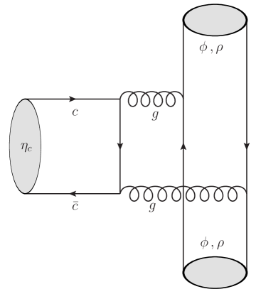
Figure 1: The schematic Feynman diagram of processes $\eta_{c}\to VV$. Here V stands for vector meson $\phi$, $\rho$, etc.

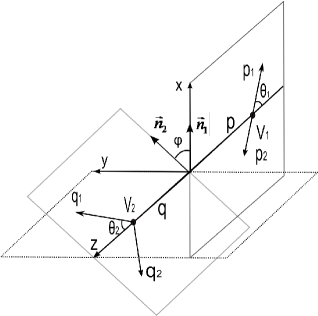
Figure 2: Relative angles and decay kinematics in the rest frame of $V_{1}$.

In quantum field theory, under the constraints of Parity conservation and Lorentz invariance the decay amplitude of $\eta_{c}\to V_{1}(p,\epsilon^{*})V_{2}(q,\epsilon^{\prime*})$, see Fig.(1,2), takes the following form

$$\mathcal{A}_{\eta_{c}\to V_{1}V_{2}}=iS\epsilon^{*\mu}\epsilon^{\prime*\nu}\varepsilon_{\mu\nu\rho\sigma}\frac{p^{\rho}q^{\sigma}}{p\cdot q}\;,$$ (2)

where $S$ is a scalar amplitude and we do not really mind its details in the aim of entanglement analysis. The above amplitude can be decomposed of the helicity amplitudes of the final states, like

$$\mathcal{A}_{\pm}=\mathcal{A}(\eta_{c}\to V_{1}(p,\epsilon^{*}_{\pm})V_{2}(q,\epsilon^{\prime*}_{\pm}))=\pm iS\;.$$ (3)

Here, we choose $q$ to be directed in positive $z$-direction in the $\eta_{c}$ rest frame, and the polarization four-vector of the light vector mesons such that in a frame where both light mesons have momentum along the $z$-axis, they are

$$\epsilon^{\prime\mu}_{\pm}=\epsilon^{\mu}_{\mp}=\frac{1}{\sqrt{2}}(0,\pm 1,i,0)\;.$$ (4)

The decay amplitude of $\eta_{c}\to V_{1}(p,\epsilon^{*})V_{2}(q,\epsilon^{\prime*})\to[P(p_{1})P(p_{2})],[P(q_{1})P(q_{2})]$ can now be expressed as

$$\frac{\mathrm{d}\Gamma_{\eta_{c}\rightarrow V_{1}V_{2}\rightarrow\ldots}}{\mathrm{d}\cos\theta_{1}\mathrm{d}\cos\theta_{2}\mathrm{d}\varphi} \propto |\sum_{\lambda=\pm 1}A_{\lambda}\epsilon_{\lambda}^{\mu}\epsilon_{\lambda}^{\prime\nu}p_{1\mu}q_{1\nu}|^{2}$$ (5)

$$= |(A_{+}\epsilon_{+}^{\mu}\epsilon_{+}^{\prime\nu}+A_{-}\epsilon_{-}^{\mu}\epsilon_{-}^{\prime\nu})p_{1\mu}q_{1\nu}|^{2}$$

$$\propto |(\epsilon_{+}^{\mu}\epsilon_{+}^{\prime\nu}-\epsilon_{-}^{\mu}\epsilon_{-}^{\prime\nu})p_{1\mu}q_{1\nu}|^{2}$$

$$\propto |\langle\vec{r}_{p_{1}}|\langle\vec{r}_{q_{1}}|\Psi\rangle|^{2}\;,$$

with

$$|\Psi\rangle = \frac{1}{\sqrt{2}}(|\epsilon_{1}^{\mu}\rangle|{\epsilon^{\prime}}_{2}^{\nu}\rangle-|\epsilon_{2}^{\mu}\rangle|{\epsilon^{\prime}}_{1}^{\nu}\rangle)\;,$$ (6)

$$\vec{r}_{p_{1}} = (\sin\theta_{1},0,-\cos\theta_{1})=(\sin\theta_{1}\vec{n}_{1},-\cos\theta_{1})\;,$$ (7)

$$\vec{r}_{q_{1}} = (\sin\theta_{2}\cos\varphi,\sin\theta_{2}\sin\varphi,\cos\theta_{2})$$ (8)

$$= (\sin\theta_{2}\vec{n}_{2},\cos\theta_{2})\;.$$

Here, $\epsilon_{1}^{\mu}=(0,1,0,0)\;,\;\epsilon_{2}^{\nu}=(0,0,1,0)$; $\vec{n}_{1,2}$ are unit vectors in the $x$-$y$ plane projected by $\vec{r}_{1,2}$; $\theta_{1,2}$ both range from $0$ to $\pi$; $\varphi$ ranges from $0$ to $2\pi$, as shown in Fig.(2). Obviously, the wave function $|\Psi\rangle$ composed of two transverse polarization vectors is an entangled state.

Integrating over $\theta_{1,2}$ we have

$$\frac{\mathrm{d}\Gamma_{\eta_{c}\rightarrow V_{1}V_{2}\rightarrow\ldots}}{\mathrm{d}\varphi} \propto |\langle\vec{n}_{1}|\langle\vec{n}_{2}|\Psi\rangle|^{2}\;,$$ (9)

$$P(\vec{n}_{1},\vec{n}_{2}) \equiv |\langle\vec{n}_{1}|\langle\vec{n}_{2}|\Psi\rangle|^{2}\;,$$ (10)

where (10) is the QM definition of the probability of one particle polarized in direction $\vec{n}_{1}$ and the other in direction $\vec{n}_{2}$.

II.2 The test of Bell inequality

We have got the QM prediction for the probability $P(\vec{n}_{1},\vec{n}_{2})$ (i.e., Eq.(10)). In the following we show that these predictions violate the Bell inequality imposed by LHVTs. To proceed the analysis, we first reformulate the entangled state of (6) in a more compact form. Further observations of Eq.(6) indicate that it describes the wave function similar to that of entangled photon pairs in Bohm .

Because of the rotation invariance about $z$-axis, we can write Eq.(6) in the following form

$$|\Psi\rangle=\frac{1}{\sqrt{2}}(\,|\epsilon(\varphi)\rangle_{V_{1}}|\epsilon(\varphi_{\perp})\rangle_{V_{2}}-|\epsilon(\varphi_{\perp})\rangle_{V_{1}}|\epsilon(\varphi)\rangle_{V_{2}})\;,$$ (11)

where $\epsilon(\varphi)$ is polarization vector in direction $\varphi$ (see Fig.(2)), and $\varphi_{\perp}=\varphi+\frac{\pi}{2}$. Since the transverse polarization of vector meson has two degrees of freedom, from (11) we can infer that if $V_{1}$ is polarized along the direction $\varphi$, the polarization of $V_{2}$ is then determined simultaneously: it must be polarized perpendicular to that of $V_{1}$.

Suppose that the transverse polarization of the state (11) is completely specified by a set of parameters $\lambda$, and the probabilities of a count being triggered by the decays of $V_{1},V_{2}$ polarizing along $\vec{n}_{1}$ and $\vec{n}_{2}$ are $p(\vec{n}_{1},\lambda)$ and $q(\vec{n}_{2},\lambda)$, respectively. According to LR, the joint probability of particle $V_{1}$ polarizing along $\vec{n}_{1}$ and particle $V_{2}$ in $\vec{n}_{2}$ is given by

$$P(\vec{n}_{1},\vec{n}_{2})=\int p(\vec{n}_{1},\lambda)q(\vec{n}_{2},\lambda)\rho(\lambda)\,\mathrm{d}\lambda\;,$$ (12)

and the single side probabilities are

$$P(\vec{n}_{1})=\int p(\vec{n}_{1},\lambda)\rho(\lambda)\,\mathrm{d}\lambda\;,$$ (13)

$$P(\vec{n}_{2})=\int q(\vec{n}_{2},\lambda)\rho(\lambda)\,\mathrm{d}\lambda\;,$$ (14)

where $\int\rho(\lambda)\,\mathrm{d}\lambda=1$. Using the simple algebraic theorem CH-inequality

$$-XY\leq xy-xy^{\prime}+x^{\prime}y+x^{\prime}y^{\prime}-x^{\prime}Y-Xy\leq 0\;,$$ (15)

where $x,x^{\prime},y,y^{\prime},X,Y$ are real numbers, and $0\leq x,x^{\prime}\leq X,0\leq y,y^{\prime}\leq Y$, and substituting $x,y$ with $p(\vec{n}_{1},\lambda),q(\vec{n}_{2},\lambda)$, setting $X,Y=1$, one can readily get the CH inequality

$$P(\vec{n}_{1},\vec{n}_{2})-P(\vec{n}_{1},\vec{n}^{\prime}_{2})+P(\vec{n}^{\prime}_{1},\vec{n}_{2})$$

$$+P(\vec{n}^{\prime}_{1},\vec{n}^{\prime}_{2})-P(\vec{n}^{\prime}_{1})-P(\vec{n}_{2}) \leq 0\;.$$ (16)

This stands as a constraint on $P(\vec{n}_{1},\vec{n}_{2})$s imposed by LR. Substituting the quantum mechanical predictions (10) into the inequality (16), we arrive at

$$\frac{1}{2}[\,\sin^{2}(\varphi_{1}-\varphi_{2})-\sin^{2}(\varphi_{1}-\varphi^{\prime}_{2})$$

$$+\sin^{2}(\varphi^{\prime}_{1}-\varphi_{2})+\sin^{2}(\varphi^{\prime}_{1}-\varphi^{\prime}_{2})-2\,] \leq 0\;.$$ (17)

Here, $\varphi\,$s are the azimuthal angles of the $\vec{n}\,$s. (17) is easily found to be violated while

$$\varphi^{\prime}_{1}=\varphi_{1}+\frac{\pi}{4}\;,\varphi_{2}=\varphi_{1}+\frac{5\pi}{8}\;,\varphi^{\prime}_{2}=\varphi_{1}+\frac{7\pi}{8}\;,$$ (18)

which gives $\frac{\sqrt{2}-1}{2}\leq 0$.

The inequality (16) bears no additional assumptions. However, if one adopts the no-enhancement assumption CH-inequality , the CH inequality then takes the following form

$$-P(\infty,\infty) \leq P(\vec{n}_{1},\vec{n}_{2})-P(\vec{n}_{1},\vec{n}^{\prime}_{2})$$ (19)

$$+P(\vec{n}^{\prime}_{1},\vec{n}_{2})+P(\vec{n}^{\prime}_{1},\vec{n}^{\prime}_{2})$$

$$-P(\vec{n}^{\prime}_{1},\infty)-P(\infty,\vec{n}_{2})\leq 0\;,$$

where symbol $\infty$ denotes the absence of analyzer on the corresponding side. If we further assume that $P(\vec{n}_{1},\infty)=P(\vec{n}_{1},\vec{n}_{2})+P(\vec{n}_{1},\vec{n}_{2\perp})$ torgerson ; EI-Garuccio , then (19) gives

$$P(\vec{n}^{\prime}_{1},\vec{n}_{2})\leq P(\vec{n}_{1\perp},\vec{n}_{2})+P(\vec{n}^{\prime}_{1},\vec{n}^{\prime}_{2\perp})+P(\vec{n}_{1},\vec{n}^{\prime}_{2})\;.$$ (20)

Here, $\vec{n}_{1\perp},\vec{n}^{\prime}_{2\perp}$ are the orthogonal directions to $\vec{n}_{1},\vec{n}^{\prime}_{2}$, and their azimuthal angles satisfy

$$\varphi_{1\perp}=\varphi_{1}+\frac{\pi}{2}\;;\;\varphi^{\prime}_{2\perp}=\varphi^{\prime}_{2}+\frac{\pi}{2}\;.$$ (21)

Similar as (17), inputting the quantum mechanical results into inequality (20), we have

$$\frac{1}{2}\{\sin^{2}(\varphi^{\prime}_{1}-\varphi_{2})-[\cos^{2}(\varphi_{1}-\varphi_{2})$$

$$+\cos^{2}(\varphi^{\prime}_{1}-\varphi^{\prime}_{2})+\sin^{2}(\varphi_{1}-\varphi^{\prime}_{2})]\} \leq 0\;,$$ (22)

which is numerically equivalent to inequality (17), and it is also violated by quantum mechanics while

$$\varphi^{\prime}_{1}=\varphi_{1}+\frac{\pi}{4}\;,\varphi_{2}=\varphi_{1}+\frac{5\pi}{8}\;,\varphi^{\prime}_{2}=\varphi_{1}+\frac{7\pi}{8}\;.$$ (23)

It is noteworthy that there are some differences between inequality (16) and (20). The (16) is an inhomogeneous one which contains both coincidence and single probabilities, while (20) is a homogeneous one which is merely composed of several coincidence probabilities santos-a . From a practical point of view, the homogeneous inequality allows test involving only coincidence counting rates. The inequality will be insensitive to many scale factors like detector efficiencies in this case and is extremely convenient for practical experiment. However the derivation of homogeneous inequalities requires additional assumptions besides locality and realism santos-a ; homoge , for more discussions of this issue we refer to a recent work homoge .

In the experiment, given that the four final pseudoscalars move with momenta $p_{1},p_{2},q_{1},q_{2}$, the azimuthal angle $\varphi$ between two decay planes of the entangled vector meson pair equals to the angle between $\vec{n}_{1}$ and $\vec{n}_{2}$, as shown in Fig.(2). The magnitudes of $P(\vec{n}_{1},\vec{n}_{2})$ in the CH inequality are therefore experimentally measurable, which is obviously the probability density, up to an overall normalization factor $\xi$, from the definition of $P(\vec{n}_{1},\vec{n}_{2})$. That is

$$P(\vec{n}_{1},\vec{n}_{2})/\xi_{p}=N^{\prime}(\varphi)/(\xi_{n}\cdot N)\;.$$ (24)

Here, $\xi_{p}$ and $\xi_{n}$ satisfy the following normalization condition

$$\int_{0}^{2\pi}\int_{0}^{2\pi}P(\vec{n}_{1},\vec{n}_{2})\,\frac{\mathrm{d}\vec{n}_{1}}{\sqrt{\xi_{p}}}\frac{\mathrm{d}\vec{n}_{2}}{\sqrt{\xi_{p}}} = 1\;,$$ (25)

$$\int_{0}^{2\pi}\int_{0}^{2\pi}N^{\prime}(\varphi)/N\,\frac{\mathrm{d}\vec{n}_{1}}{\sqrt{\xi_{n}}}\frac{\mathrm{d}\vec{n}_{2}}{\sqrt{\xi_{n}}} = 1\;,$$ (26)

with

$$N^{\prime}(\varphi) = \frac{N(\varphi+\Delta\varphi)-N(\varphi)}{\Delta\varphi}\;,$$ (27)

where $N(\varphi)$ is the event number within azimuthal angle $\varphi$ – the angle between $\vec{n}_{1}$ and $\vec{n}_{2}$, $N$ is the total event number. Eq.(24) can be expressed in a more simpler form

$$P(\vec{n}_{1},\vec{n}_{2}) = \kappa\cdot N^{\prime}(\varphi)/N\;.$$ (28)

where $\kappa=\xi_{p}/\xi_{n}$. It can be easily obtained that $\kappa=\frac{\pi}{2}$, because in computing an isolated probability $P(\vec{n}_{1},\vec{n}_{2})$, the LR models should give the same results as quantum mechanics. And, it can be seen from Eq.(11) that there will be two possible outcomes ($\varphi,\varphi_{\perp}$) if a polarization analyzed decay process happened, thus the single side probability $P(\vec{n}_{1,2})$ can be measured through

$$P(\vec{n}_{1,2})=\frac{N^{\prime}(\varphi_{1,2})}{N^{\prime}(\varphi_{1,2})+N^{\prime}(\varphi_{1,2}+\pi/2)}\;.$$ (29)

In the above expressions, apart from the constant $\kappa$, the right hand sides of Eqs. (28) and (29) are experimentally measurable, i.e., $N^{\prime}(\varphi)/N$ is the differential decay width of $\eta_{c}$ to four pseudoscalar mesons divided by its total width via intermediate vector mesons. Inputting the experimental results of (28) and (29) in the configuration of (18) into (16), one may in principle find the incompatibility of quantum theory with LR. However, in practice, to perform the test of incompatibility the experiment efficiency should be taken into account. The general inequality efficiency and background levels were once discussed by Eberhard Eberhard-ineq , and for the wave function (11) the violation of inequality (16) yields the threshold efficiency $\eta>82.8\%$ Brunner-Simon .

To carry out the test of Bell type inequality, the decay angles $\varphi$s should generally be chosen actively by experimenters, but this is not the case for mesons due to the passive character of their decays. Thus, here only a restricted class of LR can be tested Tsubasa-Izumi . A genuine Bell test also requires the decay events of two vector mesons $V_{1}$ and $V_{2}$ to be space-like separated. For the strongly decayed vector mesons ($\phi,\rho$, etc.), it is difficult to spatially distinguish the vertexes between them. Thus one can not guarantee for each particular event of $\eta_{c}\to VV\to(PP)(PP)$ that the decays of the two vector mesons are separated space-likely. However, one can obtain the fraction of space-like separation events over the total events. Given $x_{1}$ and $x_{2}$ the distance (in $\eta_{c}$ rest frame) from the $\eta_{c}$ decay point to the decay points of two $\phi$s (or $(\rho\rho)$, etc.), the space-like condition is tor-foud

$$\frac{1}{k}\leq\frac{x_{1}}{x_{2}}\leq k\;,$$ (30)

where $k=\frac{1+\beta_{V}}{1-\beta_{V}}$, $\beta_{V}=\frac{v_{V}}{c}=\sqrt{1-1/\gamma^{2}}$, $\gamma=E_{V}/m_{V}=E_{\eta_{c}}/2m_{V}$. The fraction of the space-like separated decay events to total events of the vector meson pairs is

$$\text{F}=\int_{0}^{\infty}e^{-x_{2}}\,\mathrm{d}x_{2}\int_{\frac{1}{k}x_{2}}^{kx_{2}}e^{-x_{1}}\,\mathrm{d}x_{1}=\frac{k-1}{k+1}\;.$$ (31)

Obviously, the fraction F equals to $\beta_{V}$ tor-foud . For the space-like events, constraint imposed on $P(\vec{n}_{1},\vec{n}_{2})$s by the restricted class of local realism is given by inequality (16), where the upper limit is zero. As for the non-space-like(time-like) events, the upper limit of the left hand side of (16) can maximally amount to $1/2$. In the mixture of space-like and non space-like events with ratios of $\beta_{V}$ and $1-\beta_{V}$, the upper limit of the left hand side of (16) is Tsubasa-Izumi

$$0\cdot\beta_{V}+\frac{1}{2}\cdot(1-\beta_{V})\;.$$ (32)

Therefore, to carry out the test of local realism the lower bound for the ratio $\beta_{V}$ is $\geq 2-\sqrt{2}$.

Specifically, the processes $\eta_{c}\to\phi\phi$ and $\eta_{c}\to\rho\rho$ are well-established, and the subsequent two body decays of them are

$$\phi\to K^{+}K^{-}(K_{L}^{0}K_{S}^{0})\;,\;\rho\to\pi\pi\;,$$ (33)

with large branching fractions: $\phi\rightarrow K^{+}K^{-}(K_{L}^{0}K^{0}_{S})$ $\sim 49.2\pm 0.6\%\,(34.0\pm 0.5\%)$ and $\rho\rightarrow\pi\pi$ $\sim 100\%$ PDG . The magnitudes of $\beta_{V}$ for $\phi(1020)$ and $\rho(770)$ in $\eta_{c}$ decay are $\beta_{\phi}=0.729$ and $\beta_{\rho}=0.856$, which are both larger than the lower bound of $2-\sqrt{2}\approx 0.586$.

III The polarization correlation emerged in $B\rightarrow V_{1}V_{2}$

Now we turn to the polarization correlation of the vector mesons in $B$ meson exclusive weak decays, that is $B\to V_{1}V_{2}$. There is special interest in the analysis of this process, because it is well-known that the parity is violated in the weak interaction.

The full angular dependence of the cascade decay where both vector mesons decay into pseudoscalar particles is given by bvv

$$\frac{\mathrm{d}\Gamma_{B\rightarrow V_{1}V_{2}\rightarrow\cdots}}{\mathrm{d}\cos\theta_{1}\mathrm{d}\cos\theta_{2}\mathrm{d}\varphi}\propto$$

$$|\mathcal{A}_{0}|^{2}\cos^{2}\theta_{1}\cos^{2}\theta_{2}+\frac{1}{4}\sin^{2}\theta_{1}\sin^{2}\theta_{2}(|\mathcal{A}_{+}|^{2}+|\mathcal{A}_{-}|^{2})$$

$$-\frac{1}{4}\sin 2\theta_{1}\sin 2\theta_{2}[\mathrm{Re}(e^{-i\varphi}\mathcal{A}_{0}\mathcal{A}^{*}_{+})+\mathrm{Re}(e^{+i\varphi}\mathcal{A}_{0}\mathcal{A}^{*}_{-})]$$

$$+\frac{1}{2}\sin^{2}\theta_{1}\sin^{2}\theta_{2}\mathrm{Re}(e^{+2i\varphi}\mathcal{A}_{+}\mathcal{A}^{*}_{-})$$ (34)

where $\mathcal{A}_{0,\pm}$ are the helicity amplitudes. Five observables corresponding to three amplitudes and two relative phases of the helicity amplitudes are well defined. The typical set of observables consists of the branching fraction, two out of the three polarization fractions $f_{L},f_{\parallel},f_{\perp}$, and two phases $\phi_{\parallel},\phi_{\perp}$, where

$$f_{L,\parallel,\perp}=\frac{|\mathcal{A}_{0,\parallel,\perp}|^{2}}{|\mathcal{A}_{0}|^{2}+|\mathcal{A}_{\parallel}|^{2}+|\mathcal{A}_{\perp}|^{2}}\;,\;\phi_{\parallel,\perp}^{B}=\mathrm{arg}\,\frac{\mathcal{A}_{\parallel,\perp}}{\mathcal{A}_{0}}\;$$ (35)

with

$$\mathcal{A}_{\parallel}=\frac{\mathcal{A}_{+}+\mathcal{A}_{-}}{\sqrt{2}}\;;\;\mathcal{A}_{\perp}=\frac{\mathcal{A}_{+}-\mathcal{A}_{-}}{\sqrt{2}}\;.$$ (36)

One can then obtain the azimuthal angle dependence from the subsequent decays of $V_{1}$ and $V_{2}$.

In $B$ decays, integrating over $\theta_{1}$ and $\theta_{2}$, the Eq.(34) becomes

$$\frac{\mathrm{d}\Gamma_{B\rightarrow V_{1}V_{2}\rightarrow\ldots}}{\mathrm{d}\varphi}\propto\frac{4}{9}(|\mathcal{A}_{0}|^{2}+|\mathcal{A}_{+}e^{i\varphi}+\mathcal{A}_{-}e^{-i\varphi}|^{2})$$ (37)

$$= \frac{4}{9}(|\mathcal{A}_{0}|^{2}+2|\mathcal{A}_{\parallel}\cos\varphi+i\mathcal{A}_{\perp}\sin\varphi|^{2})\;.$$

Substituting (35) into (37), we have

$$\frac{\mathrm{d}\Gamma_{B\rightarrow V_{1}V_{2}\rightarrow\ldots}}{\mathrm{d}\varphi}\propto(1+\cos 2\varphi\cdot(f_{\parallel}-f_{\perp})$$

$$+2\sin 2\varphi\sin(\phi_{\parallel}-\phi_{\perp})\sqrt{f_{\parallel}f_{\perp}})\;.$$ (38)

Taking the same procedure as introduced in Section 2.2, we have

$$P(\vec{n}_{1},\vec{n}_{2}) = \frac{1}{4}(\frac{2\pi\cdot\mathrm{d}\Gamma_{B\rightarrow V_{1}V_{2}\rightarrow\ldots}}{\mathrm{d}\varphi\cdot\Gamma_{B\rightarrow V_{1}V_{2}\rightarrow\ldots}}-f_{L})$$ (39)

$$= \frac{1}{4}(f_{\parallel}+f_{\perp}+\cos 2\varphi\cdot(f_{\parallel}-f_{\perp})$$

$$+2\sin 2\varphi\cdot\sin(\phi_{\parallel}-\phi_{\perp})\cdot\sqrt{f_{\parallel}f_{\perp}})\;,$$

where $\varphi$ is the azimuthal angle between $\vec{n}_{1}$ and $\vec{n}_{2}$.

The observables in (39) are obtainable in the experiment. For instance, in the experiment the process $B^{0}\rightarrow\phi K^{0*}$ tells b0-phik : $f_{L}=0.52\pm 0.05\pm 0.02$, $f_{\perp}=0.22\pm 0.05\pm 0.02$, $f_{\parallel}=1-f_{L}-f_{\perp}=0.26$, $\phi_{\parallel}=2.34$, $\phi_{\perp}=2.47$. Hence, the $P(\vec{n}_{1},\vec{n}_{2})$ in (39) reads

$$P(\varphi_{1},\varphi_{1}+\varphi) = \frac{1}{4}(0.48+0.04\cos 2\varphi$$

$$-2\cdot 0.24\cdot\sin 2\varphi\sin(0.13))\;.$$

Obviously, the polarization correlation is suppressed in this case due to the reasons of $f_{\parallel}\approx f_{\perp}$ and $\phi_{\parallel}\approx\phi_{\perp}$.

IV Summary and Concluding Remarks

In this work we have investigated the EPR-like correlations of the entangled vector meson pair in $\eta_{c}$ and $B$ decays. Contrary to the measurement of correlation function of polarization, which were suggested to perform in the processes of $e^{+}e^{-}\to\Lambda\bar{\Lambda}$ and $e^{+}e^{-}\to\tau^{-}\tau^{-}$, the CH inequality for the experimental test proposed in this work involves only the probabilities of transverse polarization states of the vector mesons. This reaps the benefit of the boost invariance of transverse polarization along the momentum direction of any one of the two vector mesons in $\eta_{c}$ rest frame. The probabilities in the CH inequality are shown to be experimentally measurable through subsequent two-body decays of the vector mesons, $\phi$, $\rho$, etc. Since the measurements on $\phi$ or $\rho$ to two-pseudoscalar decays are well established in the experiment, and all these decays possess large branching fractions, the $P\to VV$ processes therefore enable us to perform the test of local realism in current running colliders.

It should be mentioned that the passive character of the particle decays and the non-space-like decay events may induce restrictions on the LR models being tested and the so-called locality loophole to the experiment, which hinder the proposed test to refute the LR definitly. Nevertheless, the experimental realization of the proposals in this work may extend the test of nonlocality into the high energy regime with high dimensions, which will give us a more explicit conclusion in comparison with that from bipartite qubit case.

Moreover, taking into account proposals tor-foud and ee-tau , the experimental tests of the Bell inequalities involving spin or polarization in elementary particle physics can now be assorted into four classes, i.e.

$$\eta_{c}\stackrel{{\scriptstyle\text{Strong}}}{{\longrightarrow}} \Lambda\bar{\Lambda} \stackrel{{\scriptstyle\text{Weak}}}{{\longrightarrow}}\pi^{-}p\;\pi^{+}\bar{p}\;,$$ (40)

$$Z^{0}(\gamma^{*})\stackrel{{\scriptstyle\text{Weak(QED)}}}{{\longrightarrow}} \tau^{-}\tau^{+} \stackrel{{\scriptstyle\text{Weak}}}{{\longrightarrow}}\pi^{-}\nu_{\tau}\;\pi^{+}\bar{\nu}_{\tau}\;,$$ (41)

$$\eta_{c}\stackrel{{\scriptstyle\text{Strong}}}{{\longrightarrow}} \phi\phi \stackrel{{\scriptstyle\text{Strong}}}{{\longrightarrow}}K\bar{K}\;K\bar{K}\;,$$ (42)

$$B\stackrel{{\scriptstyle\text{Weak}}}{{\longrightarrow}} \phi K^{*} \stackrel{{\scriptstyle\text{Strong}}}{{\longrightarrow}}K\bar{K}\;K\pi\;.$$ (43)

The (40) corresponds to the suggestion of Törnqvist tor-foud ; (41) corresponds to the proposal of Privitera et al. ee-tau ; (42) and (43) belong to ours in this work. Each of the above processes in fact undergoes two steps. The first step can be viewed as the entanglement generation process, while the second step can be interpreted as the process of spin analyzing. In those two steps, either strong or weak interaction plays the dynamical role. The four different combinations of strong and weak interactions in the two steps are exhibited in Eqs.(40)-(43). Taking into account the photonic experiment, which is dominated by electromagnetic interaction, proposals for testing Bell inequalities have been put forward in three of the four fundamental interactions. To our best of knowledge the only fundamental interaction which has not been employed to generate and detect quantum entanglement is gravity.

This work was supported in part by the National Natural Science Foundation of China(NSFC) under the grants 10821063 and 10775179, by CAS Key Project on ”$\tau$-Charm Physics(NO.KJCX2-yw-N29), by the Scientific Research Fund of GUCAS, and by the Project of Knowledge Innovation Program (PKIP) of CAS with Grant No. KJCX2.YW.W10.

References

- (1) Einstein A, Podolsky B, Rosen N. Can quantum-mechanical description of physical reality be considered complete? Phys Rev, 1935, 47: 777-780
- (2) Bell J S. On the Einstein Podolsky Rosen paradox. Physics, 1964, 1: 195-200
- (3) Clauser J F, Horne M A, Shimony A, et al. Proposed experiment to test local hidden-variable theories. Phys Rev Lett, 1969, 23:880-884
- (4) Clauser J F, Horne M A. Experimental consequences of objective local theories. Phys Rev D, 1974, 10: 526-535
- (5) Aspect A, Grangier P, Roger G. Experimental realization of Einstein-Podolsky-Rosen-Bohm Gedankenexperiment: a new violation of Bell’s inequalities. Phys Rev Lett, 1982, 49: 91-94
- (6) Aspect A, Dalibard J, Roger G. Experimental test of Bell’s inequalities using time-varying analyzers. Phys Rev Lett, 1982, 49: 1804-1807
- (7) Shih Y H, Alley C O. New type of Einstein-Podolsky- Rosen-Bohm experiment using pairs of light quanta produced by optical parametric down conversion. Phys Rev Lett, 1988, 61: 2921-2924
- (8) Ou Z Y, Mandel L. Violation of Bell’s inequality and classical probability in a two-photon correlation experiment. Phys Rev Lett, 1988, 61: 50-53.
- (9) Santos E. Critical analysis of the empirical tests of local hidden-variable theories. Phys Rev A, 1992, 46: 3646-3656
- (10) Santos E. Unreliability of performed tests of Bell’s inequality using parametric down-converted photons. Phys Lett A, 1996, 212: 10-14
- (11) Abel S A, Dittmar M, Dreiner H. Testing locality at colliders via Bell’s inequality? Phys Lett B, 1992, 280: 304-312
- (12) Rowe M A, Kielpinski D, Meyer V, et al. Experimental violation of a Bell’s inequality with efficient detection. Nature, 2001, 409:791-794
- (13) GO A. Observation of Bell inequality violation in B mesons. J Mod Opt, 2004 51: 991-998
- (14) Lipkin H J. CP violation and coherent decays of kaon pairs. Phys Rev, 1968, 176: 1715-1718
- (15) Bertlmann R A. Lecture Notes in Physics 689. Springer Berlin/Heidelberg, 2006. 1-45
- (16) Li J L, Qiao C F. Feasibility of testing local hidden variable theories in a Charm factory. Phys Rev D, 2006, 74: 076003
- (17) Shi Y. High energy quantum teleportation using neutral kaons. Phys Lett B, 2006, 641: 75-80
- (18) Shi Y, Wu Y L. measurement in quantum teleportation of neutral mesons. Eur Phys J C, 2008, 55: 477-482
- (19) Törnqvist N A. Suggestion for Einstein-Podolsky-Rosen experiments using reactions like . Found Phys, 1981, 1: 171-177
- (20) Privitera P. Decay correlations in as a test of quantum mechanics. Phys Lett B, 1992, 275: 172-180
- (21) Tixier M H, et al. (the DM2 Collaboration, LAL Orsay, LPC, Clermont, Padova, Frascati), Presentation at: Conference on Microphysical Reality and Quantum Formalism, Urbino, Italy (1985).
- (22) Baranov S P. Bell’s inequality in charmonium decays and . J Phys G: Nucl Part Phys, 2008, 35: 075002
- (23) Ding Y B, Li J L, Qiao C F. Bell Inequalities in High Energy Physics. High Ener Phys & Nucl Phys, 2007, 31: 1086-1097
- (24) Li J L, Qiao C F. New possibilities for testing local realism in high energy physics. Phys Lett A, 2009, 373: 4311-4314
- (25) Bohm D, Aharonov Y. Discussion of experimental proof for the paradox of Einstein, Rosen, and Podolsky. Phys Rev, 1957, 108: 1070-1076
- (26) Torgerson J R, Branning D, Monken C H, et al. Violations of locality in polarization-correlation measurements with phase shifters. Phys Rev A, 1995, 51:4400-4403
- (27) Garuccio A. Hardy¡¯s approach, Eberhard¡¯s inequality, and supplementary assumptions. Phys Rev A, 1995, 52: 2535-2537
- (28) Zela F D. Homogeneous and genuine Bell inequalities. Phys Rev A, 2009, 79: 022102
- (29) Eberhard P E. Background level and counter efficiencies required for a loophole-free Einstein-Podolsky-Rosen experiment. Phys Rev A, 1993, 47: R747-R750
- (30) Brunner N, Gisin N, Scarani V, et al. Detection Loophole in Asymmetric Bell Experiments. Phys. Rev. Lett, 2007, 98: 220403
- (31) Ichikawa T, Tamura S, Tsutsui I. Testing EPR locality using B-mesons. Phys Lett A, 2008, 373:39-44
- (32) Amsler C, et al. Review of Particle Physics. Phys Lett B, 2008, 667: 1
- (33) Beneke M, Rohrer J, YANG D SH. Branching fractions, polarisation and asymmetries of decays. Nucl Phys B, 2007, 774: 64-101
- (34) Aubert B, et al. Measurement of the decay amplitudes. Phys Rev Lett, 2004, 93: 231804