Simulation of complete many-body quantum dynamics using controlled quantum–semiclassical hybrids

Abstract

A controlled hybridization between full quantum dynamics and semiclassical approaches (mean-field and truncated Wigner) is implemented for interacting many-boson systems. It is then demonstrated how simulating the resulting hybrid evolution equations allows one to obtain the full quantum dynamics for much longer times than is possible using an exact treatment directly. A collision of sodium BECs with $1.5\times 10^{5}$ atoms is simulated, in a regime that is difficult to describe semiclassically. The uncertainty of physical quantities depends on the statistics of the full quantum prediction. Cutoffs are minimised to a discretization of the Hamiltonian. The technique presented is quite general and extension to other systems is considered.

The calculation of the full quantum dynamics of a many-body interacting system from the microscopic description is a long-standing “difficult” problem with potential applications in many fields of physics — if only one could make it numerically tractable. The difficulty is that the size of the Hilbert space grows exponentially with the number of particles or orbitals, while path integral Monte Carlo is foiled by the rapid appearance of random phases. How new headway against this problem can be made will be demonstrated below.

Outside of fully integrable systems or 1D, where MPS/DMRG-based methods are successful, simplified descriptions are used, e.g. mean-field theory, Bogoliubov diagonalization, long-wavelength or strong interaction expansions, and Wigner-distribution based “c-field” methodstWig ; pgpemethod ; Blakiereview . However, some interesting problems fall outside the regimes of validity of these, typically where several competing effects are important or there is a transition between regimes that require different approximations. In quantum gases this occurs with rising density when interactions between the coherent component and incoherent particles already become of essence during the evolution, but the gas is not yet dense enough for the c-field descriptions to describe it with only highly occupied modes. (See Blakiereview for a comprehensive review of c-field methods and their validity). This may occur e.g. in quenches of the gasquench , colliding BECsBECcollision ; MITexpt ; Heexpt , dynamics of the cooling and trapping, shock waves and the effects of obstaclesobstacle-shock or disorderpavloff .

This kind of dynamics is often amenable to phase-space approaches that randomly sample the full quantum dynamics, such as positive-Ppp , stochastic wavefunctionsstochwavef , and stochastic gaugesgauge . They are successful when collective behaviour is important, but interactions between individual particles are not too strong. The density matrix $\widehat{\rho}$ of the system is re-described in terms of a probability distribution $\widehat{\rho}=\int P(\vec{v})\widehat{\Lambda}(\vec{v})d\vec{v}$ of basis operators $\widehat{\Lambda}$ that is subsequently randomly sampled. These samples $\vec{v}$ are then evolved according to stochastic evolution equations that are chosen to keep the entire quantum dynamics of the microscopic description. A serious limitation is the “noise catastrophe”: After some finite time, an exponential (or faster) growth of the noise variance occurs, imposing a maximum feasible simulation time $t_{\rm sim}$deuarjpa . While some phenomena can be simulateddeuarprl ; karennacoll ; otherppcalc , an extension of $t_{\rm sim}$ is much sought-after, and will be demonstrated here.

The underlying reasons why phase-space methods can overcome the Hilbert space complexity, are that quantities of physical interest usually involve contributions from many particles, and that limited precision is sufficient if it is well controlled. As in Monte-Carlo methods, there is no need to follow the amplitudes of all possible configurations as long as one can predict physical quantities with a well-controlled uncertainty. However — and now we come to the central idea to be demonstrated here — this can be taken further: There is also no true need to actually follow the troublesome exact quantum evolution equations provided that one can still predict what they would give with a well-controlled uncertainty.

How can such a roundabout prediction be achieved? If one has at one’s disposal two, or more, independent approximate methods that produce evolution equations “${\mathcal{A}}$” and “${\mathcal{B}}$” without a noise catastrophe, but which bear sufficient resemblance to the full quantum dynamics equations “${\mathcal{Q}}$”, then hybrid equations can be constructed (possibly ad-hoc) with a continuous blending parameter $\lambda$ in a scheme resembling

$${\mathcal{H_{A}}}=(1-\lambda){\mathcal{A}}+\lambda{\mathcal{Q}}\quad;\quad{\mathcal{H_{B}}}=(1-\lambda){\mathcal{B}}+\lambda{\mathcal{Q}}.$$

whose details will be non-universal. Here $\lambda=1$ gives full quantum dynamics, and $\lambda=0$ the original approximate methods. The hybrids will still contain a noise catastrophe, but at a later time than the full quantum treatment ${\mathcal{Q}}$. Therefore, long times $t>t_{\rm sim}^{{\mathcal{Q}}}$ that are not accessible by ${\mathcal{Q}}$ will be accessible by some range of $\lambda\in[0,\lambda_{\rm max}(t)\,]$.

If a physical quantity varies smoothly, preferably monotonically, as a function of $\lambda$ for hybrid ${\mathcal{H_{A}}}(\lambda)$, then an extrapolation can be made to $\lambda=1$, based on several calculations in the accessible range $[0,\lambda_{\rm max}(t)<1\,]$. One extrapolation is not yet very convincing, however, it can be checked using the other independent hybrids ${\mathcal{H_{B}}}(\lambda),\dots$. When they all agree, one has an “interpolation between extrapolations” that is robust and much more reliable. Conceptually this step is similar to comparing results obtained using different summation techniques in diagrammatic Monte-Carlo calculationsAmherst .

The remainder of this letter will demonstrate this procedure on a system of colliding BECs (schematic shown in EPAPS ). The parameters are chosen to be close to an early experiment at MITMITexpt , but deliberately with fewer atoms, to put the system in the dilute yet Bose-stimulated regime where truncated Wigner and simple quasiparticle methods fail: An $N=1.5\times 10^{5}$ atom BEC of ${}^{23}{\rm Na}$ is prepared in an elongated magnetic trap with frequencies $20\times 80\times 80$ Hz, at a temperature low enough to discount the thermal component (not unusual in experiments). A brief Bragg laser pulse coherently imparts a velocity kick of $2v_{Q}={\rm 19.64mm/s}$ to half the atoms along the long (x) condensate axis. The speed of the kicked atoms is supersonic (sound velocity in the cloud is $\leq 3.1$ mm/s). The trap is simultaneously turned off so that the wave-packets collide freely, producing a halo of scattered atom pairs moving at speeds $\approx v_{Q}$ relative to the overall centre of mass. This scattered halo exhibits a rich behaviour, which has been the repeated focus of experimentsBECcollision ; MITexpt ; Heexpt and theoryBECcollthy-early ; BECcollthy ; plfr ; Norrie ; deuarprl ; karennacoll ; karencollcorr .

The high-density regime of a similar system has been treated in detail with c-field methods in Norrie . Bogoliubov expansions and/or a pair-creation simplification treat the spontaneous regime, or special cases when BEC evolution is negligible or speed is highly supersonicBECcollthy-early ; BECcollthy (A stochastic Bogoliubov treatment gives promising results in broader casesunpub ). However, major discrepancies between predictions for halo density and correlations arise when BEC evolution or Bose stimulation is appreciable. Correlations depend on the sizes of phase grainsNorrie , which develop a complicated and poorly understood shapeplfr ; karennacoll and dynamicsdeuarprl ; karencollcorr ; Norrie in this case. Parallels to unresolved questions in other fields of physics have been noted, such as the “HBT puzzle” in heavy ion collisionsHBTion . Trustworthy calculations that reach the end of the collision (observed in experimentsHeexpt but not reached by positive-Pdeuarprl ; karennacoll ) could shed light on all these issues.

Fig. 1 includes predictions from Gross-Pitaevskii (GP) mean field, truncated Wigner, and Positive-P calculations. The time reachable by positive-P ($t_{\rm sim}^{{\mathcal{Q}}}$) is less than a half of the collision time $t_{\rm coll}\approx 1400\mu$s, and both GP and Wigner give an error. The first does not treat scattering, while for a lattice fine enough to encompass all physics the second becomes valid only for $N\gtrsim 10^{6}$ atoms (one needs $\gtrsim{\mathcal{O}}(1)$ atoms per lattice sitetWig ). N.b. the $k$-dependent difference between $g$ and its effective lattice valuetWig is $\lesssim 3\%$ here, so it has not been corrected for.

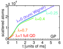
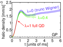
  (a)                                     (b)                                 

Figure 1: Wigner (purple), positive-P (red), GP (dashed) and hybrid ${\mathcal{H_{A}}}$ calculations at various blending parameters $\lambda$. (a): Total number of scattered atoms, from integration of k-space density (excluding the narrow BEC region). (b): Peak density of the halo (at $v_{x}=v_{z}=0$, $v_{y}=9.37$mm/s in velocity space). Triple lines show 1$\sigma$ uncertainty.

Now let us turn to obtaining the full quantum dynamics for times longer than with the positive-P. The dynamics equations in the truncated Wigner, GP, and positive-P treatments share the GP kernel with certain additions, and turn out similar enough to play the role of the ${\mathcal{A}}$, ${\mathcal{B}}$, and ${\mathcal{Q}}$.

The dynamical GP equation for the complex field $\psi({\mathbf{x}},t)$ corresponding to the cold atom Hamiltonian $\widehat{H}=\int\!d^{3}{\mathbf{x}}\,\left[\widehat{\Psi}^{\dagger}({\mathbf{x}})H_{\rm sp}({\mathbf{x}})\widehat{\Psi}({\mathbf{x}})+\frac{g}{2}\widehat{\Psi}^{\dagger}({\mathbf{x}}){}^{2}\widehat{\Psi}({\mathbf{x}})^{2}\right]$ is $i\hbar\,\dot{\psi}({\mathbf{x}})=\left[H_{\rm sp}({\mathbf{x}})+g|\psi({\mathbf{x}})|^{2}\right]\psi({\mathbf{x}})$. An initial condensate wavefunction $\phi_{GP}({\mathbf{x}})$ normalised to $\int d^{3}{\mathbf{x}}|\phi_{GP}({\mathbf{x}})|^{2}=N$ leads to initial conditions $\psi({\mathbf{x}},0)=\phi_{GP}({\mathbf{x}})$. Expectation values of observables $\langle\widehat{O}\rangle$ are calculated by making the replacements $\widehat{\Psi}\to\psi$ and $\widehat{\Psi}^{\dagger}\to\psi^{*}$ in $\widehat{O}$. For example, the density is ${\overline{n}}({\mathbf{x}})=|\psi({\mathbf{x}})|^{2}$.

In the truncated Wigner method, the dynamics is obtained by standard methods (e.g.qnoise ) based on the basis operator identities (${\mathbf{x}}$ dependence implied)

$$\widehat{\Psi}\widehat{\Lambda}=\left[\psi-\frac{1}{2}\frac{\partial}{\partial\psi^{*}}\right]\widehat{\Lambda}\ \ ;\ \ \widehat{\Psi}^{\dagger}\widehat{\Lambda}=\left[\psi^{*}+\frac{1}{2}\frac{\partial}{\partial\psi}\right]\widehat{\Lambda}$$ (1)

whose importance for us will be seen below. The equation of motion is as for GP but with the replacement $|\psi|^{2}\to(|\psi|^{2}-1)$ on the RHS. However, in the initial conditions the condensate field is admixed with half a virtual particle per mode as $\psi({\mathbf{x}},0)=\phi_{GP}({\mathbf{x}})+\eta({\mathbf{x}})/\sqrt{2}$, where $\eta({\mathbf{x}})$ is a local complex Gaussian noise with the ensemble averages $\langle\eta({\mathbf{x}})\rangle=\langle\eta({\mathbf{x}})\eta({\mathbf{x}}^{\prime})\rangle=0$ and $\langle\eta({\mathbf{x}})\eta({\mathbf{x}}^{\prime})^{*}\rangle=\delta^{3}({\mathbf{x}}-{\mathbf{x}}^{\prime})$. To calculate observables one ensemble averages a modified expression $f[\widehat{O}]$ that is obtained via $\langle\widehat{O}\rangle=\operatorname{Tr}\left[\widehat{O}\widehat{\rho}\right]=\int\!d\vec{v}P(\vec{v})\operatorname{Tr}\left[\widehat{O}\widehat{\Lambda}\right]$ and subsequent replacements (1), which give $\int\!d\vec{v}P(\vec{v})f(\vec{v})$. E.g. ${\overline{n}}({\mathbf{x}})=\langle|\psi({\mathbf{x}})|^{2}-\frac{1}{2}\rangle$.

The positive-P method uses two independent fields $\psi_{1}({\mathbf{x}},t)$ and $\psi_{2}({\mathbf{x}},t)$ and the identities

$$\begin{array}[]{r@{ = }l@{\qquad;\qquad}r@{ = }l}\widehat{\Psi}\widehat{\Lambda}&\psi_{1}\widehat{\Lambda}&\widehat{\Psi}^{\dagger}\widehat{\Lambda}&\left[\psi_{2}^{*}+\frac{\partial}{\partial\psi_{1}}\right]\widehat{\Lambda},\vspace*{1pt}\\ \widehat{\Lambda}\widehat{\Psi}^{\dagger}&\psi_{2}^{*}\widehat{\Lambda}&\widehat{\Lambda}\widehat{\Psi}&\left[\psi_{1}+\frac{\partial}{\partial\psi_{2}^{*}}\right]\widehat{\Lambda}.\end{array}$$ (2)

The $\psi_{j}$ obey the Ito stochastic equations

$$\begin{array}[]{cccc}i\hbar\dot{\psi}_{1}({\mathbf{x}})&\!\!=&\!\!\left[H_{\rm sp}({\mathbf{x}})+g\rho({\mathbf{x}})\ -\ \,\sqrt{ig}\,\xi_{1}({\mathbf{x}},t)\,\right]&\!\!\!\psi_{1}({\mathbf{x}})\\ i\hbar\dot{\psi}_{2}({\mathbf{x}})&\!\!=&\!\!\left[H_{\rm sp}({\mathbf{x}})+g\rho({\mathbf{x}})^{*}-i\sqrt{ig}\,\xi_{2}({\mathbf{x}},t)\right]&\!\!\!\psi_{2}({\mathbf{x}})\end{array}$$ (3)

with “complex density” $\rho({\mathbf{x}})=\psi_{1}({\mathbf{x}})\psi_{2}({\mathbf{x}})^{*}$. Here the $\xi_{j}$ are delta-correlated real Gaussian noise fields with the ensemble averages $\langle\xi_{j}({\mathbf{x}},t)\rangle=0$ and $\langle\xi_{i}({\mathbf{x}},t)\xi_{j}({\mathbf{x}}^{\prime},t^{\prime})\rangle=\delta_{ij}\delta(t-t^{\prime})\delta^{3}({\mathbf{x}}-{\mathbf{x}}^{\prime})$. Initial conditions are $\psi_{j}({\mathbf{x}},0)=\phi_{GP}({\mathbf{x}})$ and observables are obtained with the replacements $\widehat{\Psi}\to\psi_{1}$ and $\widehat{\Psi}^{\dagger}\to\psi_{2}^{*}$.

The next step will be to hybridize the truncated Wigner with the positive-P into treatment ${\mathcal{H_{A}}}$. It is most straightforward to proceed from hybrid operator identities for an off-diagonal expansion

$$\begin{array}[]{r@{ = }l@{\ ;\ }r@{ = }l}\widehat{\Psi}\widehat{\Lambda}&\left[\psi_{1}-\frac{1-\lambda}{2}\frac{\partial}{\partial\psi_{2}^{*}}\right]\widehat{\Lambda}&\widehat{\Psi}^{\dagger}\widehat{\Lambda}&\left[\psi_{2}^{*}+\frac{1+\lambda}{2}\frac{\partial}{\partial\psi_{1}}\right]\widehat{\Lambda}\vspace*{1pt}\\ \widehat{\Lambda}\widehat{\Psi}^{\dagger}&\left[\psi_{2}^{*}-\frac{1-\lambda}{2}\frac{\partial}{\partial\psi_{1}}\right]\widehat{\Lambda}&\widehat{\Lambda}\widehat{\Psi}&\left[\psi_{1}+\frac{1+\lambda}{2}\frac{\partial}{\partial\psi_{2}^{*}}\right]\widehat{\Lambda}\end{array}$$ (4)

One obtains: ${\overline{n}}({\mathbf{x}})=\langle\psi_{1}({\mathbf{x}})\psi_{2}({\mathbf{x}})^{*}-\frac{1-\lambda}{2}\rangle$ and initial $\psi_{j}({\mathbf{x}},0)=\phi_{GP}({\mathbf{x}})+\eta({\mathbf{x}})\sqrt{\frac{1-\lambda}{2}}$. The usual truncated-Wigner-like discarding of high-order derivatives in the relevant Fokker-Planck equations, gives dynamics

$$\begin{array}[]{cccc}i\hbar\dot{\psi}_{1}({\mathbf{x}})&\!\!=&\!\!\left[H_{\rm sp}({\mathbf{x}})+g\rho^{\prime}({\mathbf{x}})\ -\ \,\sqrt{ig\lambda}\,\xi_{1}({\mathbf{x}},t)\right]&\!\!\!\psi_{1}({\mathbf{x}})\\ i\hbar\dot{\psi}_{2}({\mathbf{x}})&\!\!=&\!\!\left[H_{\rm sp}({\mathbf{x}})+g\rho^{\prime}({\mathbf{x}})^{*}-i\sqrt{ig\lambda}\,\xi_{2}({\mathbf{x}},t)\right]&\!\!\!\psi_{2}({\mathbf{x}})\end{array}$$

with $\rho^{\prime}({\mathbf{x}})=\rho({\mathbf{x}})+\lambda-1$. As an aside, this corresponds to a representation based on an off-diagonal operator basis using $s$-orderedsorder coherent-like states with $s=\lambda$ (See EPAPS for details). Fig. 1 shows the performance of this hybrid for several values of $\lambda$ for two halo quantities of interest. As desired, $\lambda<1$ calculations last for longer than the full quantum dynamics. Here the simulation time scales as $t_{\rm sim}\approx\propto 1/\lambda$, but this is not universal.

Hybridization of the GP and positive-P methods into treatment ${\mathcal{H_{B}}}$ simply entails replacing $\sqrt{ig}$ by $\sqrt{ig\lambda}$ in the equations (3) and following the positive-P prescription from then on. Here $t_{\rm sim}\propto 1/\lambda^{2}$.

With hybrids in hand, extrapolations of the total number of scattered atoms to the full QD limit $\lambda=1$ are shown in Fig. 2 for several times $\geq t_{\rm sim}^{{\mathcal{Q}}}$. Halo peak density is inEPAPS .

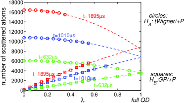
Figure 2: $\lambda$-dependent predictions for several times $\geq t_{\rm sim}^{{\mathcal{Q}}}$ (symbols) and corresponding quadratic fits (dashed line). Fitting is via minimisation of rms deviation in units of $1\sigma$ data uncertainty. Data points use $\approx 300-1000$ trajectories.

An issue here is deciding upon a fitting function – linear, quadratic, otherwise? Firstly, an acceptable fit must not have any statistically significant mismatch with the data. Secondly, to exclude spurious ill-conditioned parameters, one should choose a fit that minimises the uncertainty in the extrapolated value at $\lambda=1$ (see below). One must also beware of possible stiffness in the unseen $\lambda$, and sensitivity to this is the primary reason why several independent hybrids are needed. Details of Fig. 2 are consistent with a lack of stiffness in the unsimulated large $\lambda$ region: Firstly, for $t$ at which the whole $\lambda$ sequence is seen, there are no inflections. Secondly, the two hybrids approach the $\lambda=1$ value from different sides but agree. Also, extrapolations from only a low-$\lambda$ portion of the available data should agree with ones that use the whole sequence. This is confirmed in EPAPS .

Agreement between the ${\mathcal{H_{A}}}$ and ${\mathcal{H_{B}}}$ extrapolations in Fig. 2 is rather good at long times, but it remains to provide a well-defined uncertainty for the final prediction. Methods to obtain the statistical uncertainty of the $\lambda=1$ extrapolation are knownnumericalrecipes . In this endeavour it is very helpful to know the underlying distribution of the data points $v(\lambda)$, which are ensemble averaged observables. Conveniently, it is known to be Gaussian by the central limit theorem, and the shown 1$\sigma$ uncertainty $\Delta v(\lambda)$ is its standard deviation. One rather simple way to proceed is to generate a number $N_{S}\gg 1$ of “synthetic” data sets, where in the $j$th set one generates $v_{j}(\lambda)=v(\lambda)+\xi_{j}(\lambda)\Delta v(\lambda)$, with $\xi_{j}$ being Gaussian random variables of variance 1, mean zero. The synthetic data $v_{j}$ are distributed with the same mean as the original $v$ but double the variance. Now one calculates an extrapolated QD prediction $v_{j}(1)$ for $\lambda=1$ for each synthetic set $j$, and uses the distribution of these $v_{j}(1)$ to obtain the final uncertainty $\Delta v(1)$. Predictions from ${\mathcal{H_{A}}}$ and ${\mathcal{H_{B}}}$ that match within statistical uncertainty are trustworthy to this accuracy. The final predictions from both hybrid methods for the number of scattered atoms are shown in Fig. 3, and for halo density in EPAPS .

Figure 3: Predictions of from hybrids ${\mathcal{H_{A}}}$ and ${\mathcal{H_{B}}}$ compared with short-time full quantum dynamics and approximate methods. Triple lines, where visible, are $1\sigma$ uncertainty. Uses $\approx 10-20$ values of $\lambda$, as per Fig. 2.

One sees that the useful simulation time has been extended several-fold, allows one to reach the end of the collision here, and determine the total scattered atoms to be $8800\pm 400$ (at $t$=1.7ms). The much worse precision of the ${\mathcal{H_{A}}}$ result stems from the inherent vacuum noise in Wigner calculations and shorter segment of $\lambda$ values. However, for halo density, it is ${\mathcal{H_{B}}}$ that is more noisy.

Regarding limits of applicability, at very long times the uncertainty becomes excessive for all hybrids since the short $\lambda$ intervals give badly conditioned extrapolations. Hence the bare simulation time in the ${\mathcal{Q}}$ treatment must not be too small to ensure a sufficiently long $\lambda$ interval. It is also crucial that the blending $\lambda$ enter the dynamics in a global way: Artificial boundariespgpemethod ; scotthoffmann could make observables depend stiffly on the boundary position. For cold gases low densities can be treated perturbatively, while at high enough densities c-field treatments are valid, so that one expects that the blending method will be most useful at intermediate densities that “fall through the cracks” between these two methods. The relative simplicity of not requiring a projection onto low-energy modes may also make blending appealing in other regimes.

Finally, while the emphasis has been on cold boson dynamics, the general equation-blending approach should be broadly applicable. For hard-core boson or fermion systems other approximations would have to be hybridised with a different complete phase-space description ${\mathcal{Q}}$. One can also hybridise “imaginary-time” evolution for thermal equilibrium states, or Monte-Carlo path-integrals with the aim of predicting the ab-initio result for longer $\beta=1/T$ than is normally allowed by the fermion sign problem.

Concluding, it has been demonstrated how the full quantum dynamics of a macroscopic interacting 3D system can be calculated for much longer times than was possible with the previously most effective method, the positive-P representation. Quantitative predictions for BEC collisions in the dilute stimulated regime were obtained. The hybrid dynamical equations used, while not actually simulating complete quantum dynamics per se, can be used to confidently predict the full quantum dynamics (within a given accuracy) when several families of hybrids are available.

Supplementary material

.1 The BEC collision

(a)                                                                  

(b)                                                                  

The system simulated. (a): Schematic of the BEC collision in real space in the lab frame. (b): Slice of the velocity distribution $\rho$ in the center-of-mass frame at $v_{z}=0$ and $t=670\mu$s calculated using the positive-P method. This is about a third of the collision time, and the maximum time achievable with that method. The condensates are located around $v_{x}=\pm v_{Q}=\pm 9.82$mm/s. The halo of scattered atoms is clearly seen, as are the coherent frequency doubling peaks at $\pm 3v_{Q}\approx 30$mm/s. The collision is along the $x$ axis.

.2 The relationship of the hybrid ${\mathcal{H_{A}}}$ to $s$-ordered operators

First, a brief exposition of the standard formalism used in deriving phase-space quantum dynamics will be necessary. Writing the state of the system as a density matrix $\widehat{\rho}$, it can also be expressed as a distribution

$$\widehat{\rho}=\int d\vec{v}P(\vec{v})\widehat{\Lambda}(\vec{v}).$$ (5)

over a family of basis operators $\widehat{\Lambda}(\vec{v})$ parameterised by variables in the set $\vec{v}$. If the distribution $P(\vec{v})$ is real and non-negative, this corresponds, in turn, to an ensemble of ${\mathcal{S}}$ sets of random variables $\vec{v}$ (“configurations”) chosen according to the distribution $P$, in the limit when ${\mathcal{S}}\to\infty$. In practice one computes a finite but large ensemble (${\mathcal{S}}\gg 1$) and knows properties of $\widehat{\rho}$ to within a statistical uncertainty that can be confidently estimated from the properties of the finite ensemble.

The dynamics of the system is described by the master equation

$$i\hbar\frac{\partial\widehat{\rho}}{\partial t}=\left[\widehat{H},\widehat{\rho}\right],$$ (6)

while expectation values of observables are

$$\langle\widehat{O}\rangle=\operatorname{Tr}\left[\widehat{O}\widehat{\rho}\right].$$ (7)

These are most readily related to the computational ensemble of random variables through the use of the “operator identities”, that are specific to each formulation.

For example, in the positive-P method one chooses $\widehat{\Lambda}$ to be an off-diagonal coherent-state operator. Letting ${\mathbf{x}}$ label discrete points in the computational lattice with $\Delta V$ volume per point, defining

$$\alpha_{j}({\mathbf{x}})=\psi_{j}({\mathbf{x}})/\sqrt{\Delta V},$$

one has

$$\widehat{\Lambda}_{PP}(\vec{v})=\prod_{{\mathbf{x}}}\frac{|\alpha_{1}({\mathbf{x}})\rangle_{{\mathbf{x}}}\langle\alpha_{2}({\mathbf{x}})|_{{\mathbf{x}}}}{\langle\alpha_{2}({\mathbf{x}})|_{{\mathbf{x}}}|\alpha_{1}({\mathbf{x}})\rangle_{{\mathbf{x}}}},$$ (8)

where $\vec{v}=\left\{\alpha_{1},\alpha_{2}\right\}$,

$$|\alpha\rangle_{{\mathbf{x}}}=e^{-|\alpha|^{2}/2}e^{\alpha\widehat{a}^{\dagger}_{{\mathbf{x}}}}|0\rangle_{{\mathbf{x}}}$$

is a coherent state on the ${\mathbf{x}}$ lattice point with the complex amplitude $\alpha$ and anihilation operator $\widehat{a}_{{\mathbf{x}}}=\widehat{\Psi}({\mathbf{x}})\sqrt{\Delta V}$. Then, one finds (omitting ubiquitous local ${\mathbf{x}}$ dependence) the operator identities:

$$\widehat{\Psi}\widehat{\Lambda}_{PP}=\psi_{1}\widehat{\Lambda}_{PP}\quad \quad\widehat{\Psi}^{\dagger}\widehat{\Lambda}_{PP}=\left[\psi_{2}^{*}+\frac{\partial}{\partial\psi_{1}}\right]\widehat{\Lambda}_{PP}$$ ;

$$\widehat{\Lambda}_{PP}\widehat{\Psi}^{\dagger}=\psi_{2}^{*}\widehat{\Lambda}_{PP}\quad \quad\widehat{\Lambda}_{PP}\widehat{\Psi}=\left[\psi_{1}+\frac{\partial}{\partial\psi_{2}^{*}}\right]\widehat{\Lambda}_{PP},$$ ;

which are the source of the positive-P identities in the main text. Combined with (5) and (6) these allow one to obtain a partial differential equation for $P(\vec{v},t)$ that is equivalent to the full quantum evolution of $\widehat{\rho}(t)$. For the positive-P representation, this is a Fokker-Planck equation, and it corresponds exactly to the Langevin equations given in (5) of the main text Combining the identities with (7) and $\operatorname{Tr}\left[\widehat{\Lambda}_{PP}\right]=1$ one finds

$$\langle\widehat{O}\rangle=\int P(\vec{v})f_{O}(\vec{v})d\vec{v}$$

with a function $f_{O}$ that is obtained from $\widehat{O}$ via the operator identities, so that in the calculation it corresponds to an ensemble average of $f_{O}$. For example, for $\widehat{O}=\widehat{\Psi}^{\dagger}({\mathbf{x}})\widehat{\Psi}({\mathbf{x}})$, the function is $f_{O}=\psi_{2}^{*}({\mathbf{x}})\psi_{1}({\mathbf{x}})$. The initial coherent state corresponds to $P=\prod_{{\mathbf{x}},j}\delta^{(3)}(\psi_{j}({\mathbf{x}})-\phi_{GP}({\mathbf{x}}))$.

It has been shown that the Glauber-Sudarshan P distribution described by a coherent state operator basis

$$\widehat{\Lambda}_{GSP}(\psi)=\prod_{{\mathbf{x}}}|\alpha({\mathbf{x}})\rangle_{{\mathbf{x}}}\langle\alpha({\mathbf{x}})|_{{\mathbf{x}}}$$

(similar to the positive-P but diagonal) can be described as the limit of a representation over $s$-ordered basis states

$$\widehat{\Lambda}_{GSP}=\lim_{s\to 1^{-}}\widehat{\Lambda}_{s}$$

where $s$ can take on continuous values from -1 to 1, and

$$\widehat{\Lambda}_{s}(\psi)=\prod_{{\mathbf{x}}}\frac{\widehat{D}(\alpha)_{{\mathbf{x}}}\widehat{T}(0,-s)_{{\mathbf{x}}}\widehat{D}^{-1}(\alpha)_{{\mathbf{x}}}}{\operatorname{Tr}\left[\widehat{D}(\alpha)_{{\mathbf{x}}}\widehat{T}(0,-s)_{{\mathbf{x}}}\widehat{D}^{-1}(\alpha)_{{\mathbf{x}}}\right]}.$$ (9)

Here

$$\widehat{T}(0,-s)_{{\mathbf{x}}}=\frac{2}{1+s}\left(\frac{s-1}{1+s}\right)^{\widehat{a}^{\dagger}_{{\mathbf{x}}}\widehat{a}_{{\mathbf{x}}}}$$

is a kernel operator that becomes the vacuum $|0\rangle\langle 0|$ in the limit of $s\to 1^{-}$ and the local displacement operator is

$$\widehat{D}(\alpha)_{{\mathbf{x}}}=e^{\alpha({\mathbf{x}})\widehat{a}^{\dagger}_{{\mathbf{x}}}-\alpha({\mathbf{x}})^{*}\widehat{a}_{{\mathbf{x}}}}.$$

so that coherent states are $|\alpha\rangle=\widehat{D}(\alpha)|0\rangle$. It was also shown there that the Wigner distribution corresponds to $s=0$, hence a variation of $s$ from 0 to 1 looks like a good candidate to create the ${\mathcal{H_{A}}}$ hybrid formulation between truncated Wigner and positive-P. The “truncation” refers to ad-hoc removal of third order partial derivatives of the Wigner distribution $P$ in its evolution equation to make it interpretable as Langevin stochastic equations of the samples. This removal is the reason why truncated Wigner treatments do not reproduce the full quantum dynamics.

First, though, one must take into account the off-diagonality that is responsible for the difference between the Glauber-Sudarshan P and positive-P: $\widehat{\Lambda}_{PP}\neq\widehat{\Lambda}_{GSP}$. Notably one of the bases that reproduces the positive-P is

$$\widehat{\Lambda}_{PP}(\vec{v}) = \prod_{{\mathbf{x}}}\frac{\widehat{d}(\vec{v})_{{\mathbf{x}}}\widehat{T}(0,-1)_{{\mathbf{x}}}\widehat{d}^{-1}(\vec{v})_{{\mathbf{x}}}}{\operatorname{Tr}\left[\widehat{d}(\vec{v})_{{\mathbf{x}}}\widehat{T}(0,-1)_{{\mathbf{x}}}\widehat{d}^{-1}(\vec{v})_{{\mathbf{x}}}\right]}$$ (10)

$$= \prod_{{\mathbf{x}}}\widehat{d}(\vec{v})_{{\mathbf{x}}}\widehat{T}(0,-1)_{{\mathbf{x}}}\widehat{d}^{-1}(\vec{v})_{{\mathbf{x}}}$$

where the “displacement-like” operator

$$\widehat{d}(\vec{v})_{{\mathbf{x}}}=e^{\alpha_{1}({\mathbf{x}})\widehat{a}^{\dagger}_{{\mathbf{x}}}-\alpha_{2}({\mathbf{x}})^{*}\widehat{a}_{{\mathbf{x}}}}.$$

is obtained by the replacement $\alpha\to\alpha_{1},\alpha^{*}\to\alpha_{2}^{*}$ in $\widehat{D}(\alpha)$, and the second line follows because the trace in the denominator evaluates to one. The reason for this particular replacement is that for the positive-P distribution one requires $\widehat{\Lambda}$ to depend analytically on two separate complex variables, hence their complex conjugates must be removed. Here these analytic variables are $\alpha_{1}$ and $\alpha_{2}^{*}$.

The extension of this $\widehat{\Lambda}$ onto a family of $s$-ordered bases is

$$\widehat{\Lambda}_{s}^{{\mathcal{A}}}(\vec{v}) = \prod_{{\mathbf{x}}}\frac{\widehat{d}(\vec{v})_{{\mathbf{x}}}\widehat{T}(0,-s)_{{\mathbf{x}}}\widehat{d}^{-1}(\vec{v})_{{\mathbf{x}}}}{\operatorname{Tr}\left[\widehat{d}(\vec{v})_{{\mathbf{x}}}\widehat{T}(0,-s)_{{\mathbf{x}}}\widehat{d}^{-1}(\vec{v})_{{\mathbf{x}}}\right]}$$ (11)

$$= \prod_{{\mathbf{x}}}\widehat{d}(\vec{v})_{{\mathbf{x}}}\widehat{T}(0,-s)_{{\mathbf{x}}}\widehat{d}^{-1}(\vec{v})_{{\mathbf{x}}}.$$

This then interpolates towards the Wigner representation. Note that since the truncated Wigner evolution is deterministic, then if one takes the formally off-diagonal basis set with $s=0$ but imposes $\delta(\psi_{1}-\psi_{2})$ in the initial conditions, it will remain exactly equivalent to the normal truncated Wigner formulation of (9) with $s=0$.

One obtains the identities

$$\widehat{\Psi}\widehat{\Lambda}^{{\mathcal{A}}}_{s} = \left[\psi_{1}-\frac{1-s}{2}\frac{\partial}{\partial\psi_{2}^{*}}\right]\widehat{\Lambda}^{{\mathcal{A}}}_{s}$$

$$\widehat{\Psi}^{\dagger}\widehat{\Lambda}^{{\mathcal{A}}}_{s} = \left[\psi_{2}^{*}+\frac{1+s}{2}\frac{\partial}{\partial\psi_{1}}\right]\widehat{\Lambda}^{{\mathcal{A}}}_{s}$$

$$\widehat{\Lambda}^{{\mathcal{A}}}_{s}\widehat{\Psi}^{\dagger} = \left[\psi_{2}^{*}-\frac{1-s}{2}\frac{\partial}{\partial\psi_{1}}\right]\widehat{\Lambda}^{{\mathcal{A}}}_{s}$$

$$\widehat{\Lambda}^{{\mathcal{A}}}_{s}\widehat{\Psi} = \left[\psi_{1}+\frac{1+s}{2}\frac{\partial}{\partial\psi_{2}^{*}}\right]\widehat{\Lambda}^{{\mathcal{A}}}_{s}$$

which are exactly the same as was obtained by a naive blending of the operator identities in the main text provided we identify $\lambda=s$.

Regarding initial conditions, the diagonal $s$-ordered representation (9) for a coherent state $|\phi_{GP}\rangle$ was found by Cahill and Glauber to be Gaussian

$$P(\psi)=\prod_{{\mathbf{x}}}\frac{2}{1-s}\exp\left(-\frac{2|\psi({\mathbf{x}})-\phi_{GP}({\mathbf{x}})|^{2}}{\Delta V(1-s)}\right).$$ (12)

When one additionally imposes $\psi_{1}=\psi_{2}=\psi$ as is done in the main text, this is equivalent to (11), justifying the initial conditions given in the main text that contain complex Gaussian noise of variance $(1-s)/2$.

.3 Halo density calculations

$\lambda$-dependent predictions of halo density (at $v_{x}=v_{z}=0$, $v_{y}=9.37$mm/s in velocity space) for several times (circles) with uncertainty shown as vertical bars at the same location. The corresponding fits (dashed) are quadratic for the ${\mathcal{H_{B}}}$ hybrid, and constant-value for ${\mathcal{H_{A}}}$. Fitting is via minimisation of rms deviation in units of $1\sigma$ data uncertainty. Linear or quadratic fits to the ${\mathcal{H_{A}}}$ hybrid data are not more statistically significant than the constant-value fit, and hence would be poorly conditioned.

Predictions of halo density (at $v_{x}=v_{z}=0$, $v_{y}=9.37$mm/s in velocity space) from hybrids ${\mathcal{H_{A}}}$ and ${\mathcal{H_{B}}}$ compared with short-time full quantum dynamics and approximate methods. Triple lines, where visible, are $1\sigma$ uncertainty. Prediction data based on $\approx 10-20$ values of $\lambda$, each with $\approx 300-1000$ trajectories, and quadratic / constant-value fitting for ${\mathcal{H_{A}}}$ / ${\mathcal{H_{B}}}$ hybrids, respectively. Note the agreement with truncated Wigner to within statistical uncertainty. Times detailed in the previous figure (above) are highlighted.

.4 Extrapolation from partial $\lambda$ segment

Predictions of the number of scattered atoms at several times, as a function of the $\lambda$ segment $\lambda\in[0,\lambda_{\rm max}]$ used for extrapolation from a quadratic fit to ${\mathcal{H_{A}}}$ results. Triple lines, where visible, are $1\sigma$ uncertainty. Dashed lines indicate the final predictions using all the available $\lambda$ values. Data used was from the same simulations as in Fig. 2 of the main text. There is no statistically significant trend with $\lambda_{\rm max}$ visible, suggesting that the fitting function that is a quadratic polynomial in $\lambda$ is appropriate within statistical precision.