THE INCLUSIVE-EXCLUSIVE CONNECTION AND THE NEUTRON NEGATIVE CENTRAL CHARGE DENSITY

Abstract

We find an interpretation of the recent finding that the central charge density of the neutron is negative by using models of generalized parton distributions at zero skewness to relate the behavior of deep inelastic scattering quark distributions, evaluated at high $x$, to the transverse charge density evaluated at small distances. The key physical input of these models is the Drell-Yan-West relation We find that the $d$ quarks dominate the neutron structure function for large values of Bjorken $x$, where the large longitudinal momentum of the struck quark has a significant impact on determining the center-of-momentum of the system, and thus the “center” of the nucleon in the transverse position plane.

1 Outline

Electron scattering is the preferred tool for extracting information on the spatial and momentum distribution of the quarks in nucleons. High energy scattering provides a clean picture of the quarks’ momentum distribution for a nucleon boosted into infinite momentum frame (IMF). Measurements of elastic scattering at lower energy scales allow extraction of the nucleon form factors, which can be related to the spatial distribution of charge in the rest frame of the nucleon. However, obtaining rest frame charge distributions requires model-dependent relativistic boost corrections, limiting our ability to extract these distributions from data. Significant work has gone into better understanding the issues involved in studying nucleon distributions, as well as providing unified descriptions of the space and momentum distributions of the quarks.

The present discussion and the papers on which it is based would not have been possible without the great amount of experimental technique, effort and ingenuity that has been used recently to measure the electromagnetic form factors of the nucleon[1, 2, 3, 4]. These quantities are probability amplitudes that the nucleon can absorb a given amount of momentum and remain in the ground state, and are related to the nucleon charge and magnetization densities.

We note that there will be an Institute for Nuclear Theory Program held in the Fall of 2009 that is devoted to the electromagnetic physics of the Jefferson Laboratory upgrade to 12 GeV. Please see the website: www.int.washington.edu/PROGRAMS/09-03.html.

We begin our analysis by reviewing recent work[5] that determines the transverse charge density of the neutron in a model independent way. This work surprisingly found that the central charge density is negative. Then we discuss how the inclusive-exclusive connection is used to provide an interpretation for this fact[6].

2 Definitions and the density interpretation

We begin by by presenting definitions of the form factors. Let $J^{\mu}(x^{\nu})$ be the electromagnetic current operator, in units of the proton charge. Then the nucleon form factors are given by the matrix element

$$\langle p^{\prime},\lambda^{\prime}|J^{\mu}(0)|p,\lambda\rangle=\bar{u}(p^{\prime},\lambda^{\prime})\left(\gamma^{\mu}F_{1}(Q^{2})+i\frac{\sigma^{\mu\alpha}}{2M}q_{\alpha}F_{2}(Q^{2})\right)u(p,\lambda),$$ (1)

where $M$ is the nucleon mass, and the momentum transfer $q_{\alpha}=p^{\prime}_{\alpha}-p_{\alpha}$ is taken as space-like, so that $Q^{2}\equiv-q^{2}>0.$ The nucleon polarization states are chosen to be those of definite light-cone helicities $\lambda,\lambda^{\prime}$.[7] The charge (Dirac) form factor is $F_{1}$, normalized such that $F_{1}(0)$ is the nucleon charge, and the magnetic (Pauli) form factor is $F_{2}$, normalized such that $F_{2}(0)$ is the anomalous magnetic moment. The Sachs form factors are $G_{E}(Q^{2})\equiv F_{1}(Q^{2})-\frac{Q^{2}}{4M^{2}}F_{2}(Q^{2}),\;G_{M}(Q^{2})\equiv F_{1}(Q^{2})+F_{2}(Q^{2}).$

In the Breit frame, in which ${\bf p}=-{\bf p}^{\prime}$, $G_{E}$ is the nucleon helicity flip matrix element of $J^{0}$. This has been interpreted as meaning that $G_{E}$ is the three-dimensional Fourier transform of the charge density in the rest frame. Indeed, the scattering of neutrons from the electron cloud of atoms measures the derivative $-\frac{1}{6}dG_{E}(Q^{2})/dQ^{2}$ at $Q^{2}=0$, which has been widely interpreted as the mean-square charge radius of the neutron. However, a direct probability or density interpretation of $G_{E}$ is spoiled by a non-zero value of $Q^{2}$, no matter how small. This is because relativistic dynamics, which cause the wave functions of the initial and final nucleons of different momenta to differ, must be used. The final wave function is related to the initial one by a complicated boost operator that when acting on the initial state of a given momentum changes it to the same of the different final momentum. In general the boost operator (or boost) contains the effects of interactions. Thus the initial and final states differ, invalidating a probability or density interpretation. It is only in the case that non-relativistic dynamics are applicable that form factors are simply the Fourier transforms of the rest frame spatial distributions.

It has commonly been assumed that at low momentum transfers, these corrections could be safely neglected. If we treat relativistic corrections as in atomic physics, they are governed by $v^{2}/c^{2}\sim p^{2}/m^{2}$, where $m$ is the mass of the boosted constituent. Computing the form factors involves integrating over the momentum $p$ so that it is replaced by the momentum transfer $Q$. Thus for small values of $Q^{2}$ we find

$$G_{E}(Q^{2})=G_{E}(0)-{Q^{2}\over 6}\left(\int d^{3}rr^{2}\rho(r)+C/m^{2}\right),$$ (2)

where $C$ is an unknown coefficient. In a simple constituent quark model, $m\approx 300$ MeV, and so these $1/m^{2}$ boost corrections are negligible only for $p^{2}\ll 0.1$ GeV². However, for the neutron $G_{E}(0)=0$, so the corrections are expected to be relatively large. The boost correction term need not be small compared to the finite size contribution unless $C\ll 1$; since both corrections scale with $Q^{2}$, the relative correction to the extracted radius does not vanish as $Q^{2}$ approaches 0. The constituent quarks represent the low $Q^{2}$, dressed versions of the near-massless current quarks of QCD. For current quarks of mass 5–10 MeV, the boost corrections are important for all $Q^{2}$ values where measurements exist. While it is possible to construct systematically improveable models which should yield a complete description of the nucleon, it is not clear how one would quantitatively determine how well any particular model fully reproduces the corrections associated with the relativistic boost. Thus, there is always some model dependence in the extraction of the rest frame charge distributions from the form factors, and it is not clear how well one can quantify these corrections and uncertainties, even at very low $Q^{2}$.

3 Light Cone Coordinates, the Infinite Momentum Frame, and the Drell-Yan Frame

The use of light cone coordinates and the kinematic subgroup of the Poincaré group, which is closely related to the use of the infinite momentum frame, enables one to avoid the difficulties associated with including the boost.

The basic idea is that the “time” variable is given by $x^{+}=(ct+z)/\sqrt{2}=(x^{0}+x^{3})/\sqrt{2}$ and the conjugate evolution operator is given by $p^{-}=(p^{0}-p^{3})/\sqrt{2}.$ Starting in an ordinary reference frame and making a Lorentz transformation into a frame moving with nearly the speed of light in the $3$ direction converts the usual $t$ into $x^{+}$. The 3 spatial variables must be different than $x^{+}$, so we take $x^{-}=(x^{0}-x^{3})/\sqrt{2}.$ If $x^{+}=0$ then $x^{-}=-\sqrt{2}z$ and $x^{-}$ can be thought of as something like a $z$ or $x^{3}$ variable, but rotational invariance can not generally be used to relate the $x^{-}$ and $x,y$ dependence of the density. The canonically conjugate momentum to $x^{-}$ is $p^{+}=(p^{0}+p^{3})/\sqrt{2}.$ For the transverse degrees of freedom we use the usual position $(x,y)$ and momentum $(p_{x},p_{y})$ variables denoted by ${\bf b},{\bf p}$ where the boldface notation denotes a transverse vector.

We also exploit the kinematic subgroup. That is transverse Lorentz transformations, with a transverse velocity ${\bf v}$ (or boosts in the transverse $x,y$ or ${\bf b}$ direction) do not involve interactions. In particular, these transformations are defined by $k^{+}\rightarrow k^{+},{\bf k}\rightarrow{\bf k}-k^{+}{\bf v},$ with $k^{-}$ changed so that $k_{\mu}k^{\mu}$ is not changed. These transformations are just like the non-relativistic Galilei transformation except that $k^{+}$ appears instead of a mass. This means that we are allowed to do Fourier transformations of variables provided transverse degrees of freedom are involved.

If the momentum transfer vector $q^{\mu}$ is space-like we may use the so-called Drell-Yan (DY) frame in which $q^{+}=0$. This means that the plus component of the momentum of the nucleon is the same before and after the absorption of the single photon. Then the momentum transfer vector is in the transverse direction, so that usual two-dimensional Fourier transform techniques can be used.

4 Charge density of the neutron

A proper determination of a charge density requires the measurement of a density operator. We shall show that measurements of the pion form factor directly involve the three-dimensional parton charge density operator, in the infinite momentum frame IMF, $\hat{\rho}_{\infty}(x^{-},{\bf b})=J^{+}(x^{-},{\bf b})$. In this frame the electromagnetic charge density $J^{0}$ becomes $J^{+}$ and

$$\hat{\rho}_{\infty}(x^{-},{\bf b})=\sum_{q}e_{q}\overline{q}(x^{-},{\bf b})\gamma^{+}q(x^{-},{\bf b})=\sum_{q}e_{q}\sqrt{2}q^{\dagger}_{+}(x^{-},{\bf b})q_{+}(x^{-},{\bf b}),$$ (3)

where $q_{+}(x^{\mu})=\gamma^{0}\gamma^{+}/\sqrt{2}q(x^{\mu})$, the independent part of the quark-field operator $q(x^{\mu})$. We set the time variable, $x^{+}=(t+z)/\sqrt{2},$ to zero, and do not display it in any function.

The spatial structure of a hadron can be examined if one uses[8, 9, 10] states that are transversely localized. The state with transverse center of mass ${\bf R}$ set to 0 is formed by taking a linear superposition of states of transverse momentum:

$$\left|p^{+},{\bf R}={\bf 0},\lambda\right\rangle\equiv{\cal N}\int\frac{d^{2}{\bf p}}{(2\pi)^{2}}\left|p^{+},{\bf p},\lambda\right\rangle,$$ (4)

where $\left|p^{+},{\bf p},\lambda\right\rangle$ are light-cone helicity eigenstates [7] and ${\cal N}$ is a normalization factor satisfying $\left|{\cal N}\right|^{2}\int\frac{d^{2}{\bf p}_{\perp}}{(2\pi)^{2}}=1$. The expansion Eq. (4) makes sense only in the infinite momentum frame $p^{+}\rightarrow\infty$ because we must have $2p^{+}p^{-}-{\bf p}^{2}=M^{2}$. The nucleon states are normalized as $\langle{p^{\prime}}^{+},{\bf p}^{\prime}\lambda^{\prime}|{p}^{+},{\bf p},\lambda\rangle=2p^{+}(2\pi)^{3}\delta_{\lambda^{\prime},\lambda}\delta({p^{\prime}}^{+}-p^{+})\delta^{(2)}({{\bf p}}^{\prime}-{\bf p})$.

Next we relate the charge density

$${\rho}_{\infty}(x^{-},{\bf b})=\frac{\left\langle p^{+},{\bf R}={\bf 0},\lambda\right|\hat{\rho}_{\infty}(x^{-},{\bf b})\left|p^{+},{\bf R}={\bf 0},\lambda\right\rangle}{\left\langle p^{+},{\bf R}={\bf 0},\lambda|p^{+},{\bf R}={\bf 0},\lambda\right\rangle},$$ (5)

to $F_{1}(Q^{2})$. In the DY frame no momentum is transferred in the plus-direction, so that information regarding the $x^{-}$ dependence of the distribution is not accessible. Therefore we integrate over $x^{-}$, using the relationship translational invariance, and then use our momentum expansion and the definition of $F_{1}$ as the helicity non-flip matrix element of $J^{+}$ in a Drell-Yan frame to find

$$\rho(b)\equiv\int\;dx^{-}\rho_{\infty}(x^{-},b)$$ (6)

$$\rho(b)=\int\frac{d^{2}q}{(2\pi)^{2}}F_{1}(Q^{2}={\bf q}^{2})e^{-i{\bf q}\cdot{\bf b}}=\int\frac{Q\;dQ}{(2\pi)}F_{1}(Q^{2})J_{0}(Qb)e^{-i{\bf q}\cdot{\bf b}},$$ (7)

where $J_{0}$ is a cylindrical Bessel function and $\rho(b)$ is termed the transverse charge density, giving the charge density at a transverse position $b$, integrating over all longitudinal momentum. In the infinite momentum frame, the longitudinal dimension of the nucleon is contracted to a point, and only the transverse position remains. The value of $b=0$ corresponds to the center of longitudinal-momentum of the nucleon in the transverse dimension.

It is not as straightforward to isolate the magnetization distribution, and there have been multiple such densities proposed [11, 12]. Starting with the matrix element of ${\bf J}\cdot{\bf A}$ and working in the infinite momentum frame leads to the result that the transverse magnetization density to is the two-dimensional Fourier transform of $F_{2}$, just as the charge density is the transform of $F_{1}$ [11]. This interpretation yields a difference between the magnetic and electric radii in the proton.

Figure 1: Upper panel: proton transverse charge density $\rho(b)$. Lower panel: neutron transverse charge density. The solid curves use the parameterization of Kelly, and the dashed (red) curves use Bradford, et al.. Reprinted with permission from Ref. ⁵.Copyright 2007 by the American Physical Society.

Here we exploit Eq. (7) by using recent parameterizations [13, 14, 15] of measured form factors to determine $\rho(b)$. Applying Eq. (7) to the proton using two sets of form factor parameterizations[13, 14] yields the results shown in the upper panel of Fig. 1. The curves obtained using the two different parameterizations overlap. Furthermore, there is negligible sensitivity to form factors at very high values of $Q^{2}$ that are currently unmeasured. The density is peaked at low values of $b$, but has a long positive tail, suggestive of a long-ranged, positively charged pion cloud.

The neutron results for $\rho(b)$ are shown in the lower panel of Fig. 1. The curves obtained using the two different parameterizations seem to overlap, but we will return to this below. The surprising result is that the central neutron charge density is negative. The negative nature of the neutron’s central charge density appears to contradict two current ideas. If the neutron is sometimes a proton surrounded by a negatively charged pionic cloud, one would expect to obtain a positive central density[16]. Another mechanism involving correlations in the nucleonic wave function induced by one gluon exchange would also lead to a positive central density because the interaction between two identical $d$ quarks[17] is repulsive.

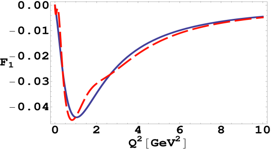
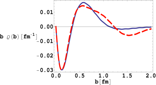
Figure 2: Neutron $F_{1}$ and transverse charge density. Upper panel: $F_{1}$. Lower panel: $b\rho(b)$ in transverse position space. The solid curves are obtained using the fits of Kelly, and the dashed curves the fits of Bradford, et al.. Reprinted with permission from Ref. ⁵. Copyright 2007 by the American Physical Society.

The resultant negative central density thus deserves further examination. The upper panel of Fig. 2 shows $F_{1}$ for the neutron obtained using the two different parameterizations[14, 13] which are observably different. However, in both cases. $F_{1}$ is negative for all values of $Q^{2}$. If $F_{1}$ is always negative, then taking $b=0,\;J_{0}(Qb)=1$ in Eq. (7), will always yield a negative central density. The long range structure of the charge density is captured by displaying the quantity $b\rho(b)$ in the lower panel of Fig. 2. At very large distances from the center, the charge density is negative, as expected in the pion cloud picture.

These findings appear to contradict previous understanding of the nucleon charge distributions based on the model-dependent extraction of the rest frame charge distributions. Because of the large and model-dependent boost corrections at large $Q^{2}$, one cannot obtain information about the rest frame charge density at the very center of the nucleon from measurements of the form factors. While there is no direct experimental information on this possibility of a very small negative core in the rest frame distribution, this negative core seems to contradict the accepted explanations of the origin of the long range negative cloud which occurs along with a positively charged interior. In addition, the negative core in the IMF transverse density is a feature even in models that build up the charge distribution based on a pion cloud model. It is clearly important to understand the differences between the IMF charge density and the rest frame charge density to fully understand the new features of these model-independent spatial distributions.

The surprising model independent result is that the density of the neutron is negative. The remainder of this presentation is concerned with trying to explain this remarkable feature of nature.

5 Inclusive-exclusive connection

Generalized parton distributions (GPDs) contain information about the longitudinal momentum fraction $x$ as well as the transverse position $b$. Information regarding the $x$ and $b$ dependence is obtained from experiment by using GPDs to reproduce both deep inelastic scattering and elastic scattering data. Thus we use this inclusive-exclusive connection to better understand the central neutron charge density.

The widely studied GPDs[18, 19] are of high current interest because they can be related to the total angular momentum carried by quarks in the nucleon. We consider the specific case in which the longitudinal momentum transfer $\xi$ is zero, and the initial and final nucleon helicities are identical ($\lambda^{\prime}=\lambda$). Then, in the light-cone gauge, $A^{+}=0$, the matrix element defining the GPD $H_{q}$ for a quark of flavor $q$ and zero skewness is

$$H_{q}(x,t)=\langle p^{+},{\bf p}^{\prime},\lambda|\widehat{O}_{q}(x,{\bf 0})|p^{+},{\bf p},\lambda\rangle,$$ (8)

where

$$\widehat{O}_{q}(x,{\bf b})\equiv\int\frac{dx^{-}}{4\pi}{q}_{+}^{\dagger}\left(-\frac{x^{-}}{2},{\bf b}\right)q_{+}\left(\frac{x^{-}}{2},{\bf b}\right)e^{ixp^{+}x^{-}}.$$ (9)

We abbreviate $H_{q}(x,\xi$=$0,t)\equiv H_{q}(x,t)$ and $-t=-(p^{\prime}-p)^{2}=({\bf p}^{\prime}-{\bf p})^{2}=Q^{2}.$

It is well known that GPDs provide a unified description of a number of hadronic properties.[18] Of particular interest here is that for $t$=0 they reduce to conventional PDFs, $H_{q}(x,0)=q(x)$, and that the integration of the charge-weighted $H_{q}$ over $x$ yields the nucleon electromagnetic form factor:

$$F_{1}(t)=\sum_{q}e_{q}\int dxH_{q}(x,t).$$ (10)

The impact parameter-dependent PDF[20] for a quark of flavor $q$ is the matrix element of the operator $\widehat{O}_{q}$ in the state $\left|p^{+},{\bf R}={\bf 0},\lambda\right\rangle$:

$$\rho_{\perp}^{q}({\bf b},x)\equiv\left\langle p^{+},{\bf R}={\bf 0},\lambda\right|\widehat{O}_{q}(x,{\bf b})\left|p^{+},{\bf R}={\bf 0},\lambda\right\rangle.$$ (11)

We use the notation $\rho_{\perp}^{q}({\bf b},x)$ instead of the originally defined[20] $q(x,{\bf b})$ because this quantity is a density that gives the probability that the quark has a longitudinal momentum fraction $x$ and is at a transverse position ${\bf b}$. The quantity $\rho_{\perp}^{q}({\bf b},x)$ is the two-dimensional Fourier transform of the GPD $H_{q}$:

$$\rho_{\perp}^{q}({\bf b},x)=\int\frac{d^{2}q}{(2\pi)^{2}}e^{-i\;{\bf q}\cdot{\bf b}}H_{q}(x,t=-{\bf q}^{2}).$$ (12)

We extract the form factor $F_{1}$ by integrating $\rho_{\perp}^{q}({\bf b},x)$ over all values of $x$, multiplying by the quark charge $e_{q}$, and summing over quark flavors $q$.[8] The result is the IMF charge density in transverse space:

$$\rho(b) \equiv\sum_{q}e_{q}\int dx\;\rho_{\perp}^{q}({\bf b},x).$$ (13)

The relations Eq. (13) and Eq. (6) provide two expressions for the transverse density $\rho(b)$. The impact parameter GPD and the three-dimensional density are related by Parseval’s theorem. The quantity $\rho(b)$ gives the charge density at a transverse position ${\bf b}$ irrespective of the longitudinal momentum fraction or longitudinal position.

There is a tight connection between the values of $x$ and the values of ${\bf b}$. For a given Fock space component, the center of transverse momentum (CM) ${\bf R}$ is given by

$${\bf R}=0=\sum_{i}x_{i}{\bf b}_{i},$$ (14)

where $x_{i},{\bf b}_{i}$ are the longitudinal momentum fractions and transverse positions of the $i$’th partons. Using this definition, the longitudinal momentum of a quark determines it’s impact on defining the transverse position of the nucleon. If the struck quark, $x_{i}$, carries nearly all of the plus component of the total momentum, then the other quarks must carry a total plus momentum of $1-x_{i}$ which approaches zero as $x_{i}\to 1$. Thus, $x_{j}\to 0$ for $i\neq j$, and via Eq. (14), ${\bf b}_{i}$ must also approach zero as long as the values of ${\bf b}_{j}$ remain finite. Thus, large values of $x$ correspond to a small value of $b$, as the struck quark plays a large role in defining the transverse center of mass as $x\to 1$.

Let us investigate $\rho_{\perp}({\bf b},x)$ to understand the origin of the neutron’s negative central charge density. The quantities are not measured directly, but have been obtained from models that incorporate fits to parton distributions and electromagnetic nucleon form factors.[21, 22, 23, 24] This method exploits form factor sum rules at zero skewness to model information regarding the valence quark GPDs, $H^{q}_{v}\equiv H^{q}-H^{\bar{q}}$. This yields the net contribution to the form factors from quarks and anti-quarks, although it does not correspond to the valence distribution within a model for which sea distributions for quarks and antiquarks have different $x$ or $t$ dependences. The effects of strangeness are neglected in these fits.

Each parameterization we use[21, 22, 23] incorporates the Drell-Yan-West[25] relationship between the behavior of the structure function $\nu W_{2}(x)$ function near $x=1$, measured in inclusive reactions and the behavior of the electromagnetic form factor at large values of $Q^{2}$, measured in the exclusive elastic scattering process. In particular, for a system of $n+1$ valence quarks, described by a power-law wave function

$$\lim_{x\rightarrow 1}\nu W_{2}(x)=(1-x)^{2n-1}\to\lim_{Q^{2}\rightarrow\infty}F_{1}(Q^{2})=\frac{1}{Q^{2n}},$$ (15)

with the relation being that the same value of $n$ that defines the high-$x$ behavior of the structure function also defines the high-$Q^{2}$ behavior of the form factor, thus associating the behavior of large values of $x$ with large momentum transfers, $Q^{2}={\bf q}^{2}$, which in turn correspond to small values of $b$. So again we see we see a connection between large values of $x$ and small values of $b$.

To proceed further we use specific forms of the GPDs, and these determine the details of the results. Diehl et al.[22] use

$$H^{q}_{v}(x,t)=q_{v}(x)\exp[f_{q}(x)t],$$ (16)

where

$$f_{q}(x)=[\alpha^{\prime}\log[1/x]+B_{q}](1-x)^{3}+A_{q}x(1-x)^{2},$$ (17)

is the form that gives the best fit to the data. The parameter $\alpha^{\prime}$ represents the slope of the Regge trajectory, and the CTEQ6 PDFs[26] are taken as input. Here we use the best fit parameters, taken from the second line of Table 8 of Ref. [22]. These are detailed in Ref. [6]. The labels $q$ refer to $u$ and $d$, the $u$ and $d$ quarks in the proton. These correspond to $d$ and $u$ quarks in the neutron, if charge symmetry  [27, 28, 29, 30] is upheld. For the proton, $2d_{v}/u_{v}$ falls rapidly for large values of $x$, which means that $u$ quarks dominate the parton distribution for large values of $x$. For the neutron, the assumption of charge symmetry implies that $d_{v}$ for the neutron is the same as $u_{v}$ for the proton, and vice-versa. Thus, the $d$ quarks dominate the parton distribution in the neutron for large values of $x$. The distributions of Ref. [21] have $A_{q}=B_{q}=0$ and $f_{q}(x)=[\alpha^{\prime}_{q}\log[1/x]](1-x).$ Those of Ref. [23] have a more complicated form and include the additional constraint that the nucleon consists of three quarks at an initial scale of $Q_{0}^{2}=0.094$ GeV².

We study the connection between regions of $x$ and regions of $b$. To do this define

$$\rho_{\perp}^{q}(b,\Delta x)\equiv\int_{\Delta x}dx~{}e_{q}~{}\rho_{\perp}^{q}(b,x),$$ (18)

where $e_{q}$ is the quark charge in units of the proton charge ($e_{u}=2/3,\;e_{d}=-1/3$) with $\rho_{\perp}^{p,n}$ being obtained from appropriate sums of $\rho_{\perp}^{q}$. This represents the contribution to the charge density from quarks in the $x$ region defined by $\Delta x$, rather than the total density obtained by integrating over all $x$.

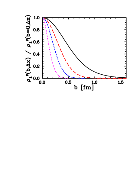
Figure 3: The proton transverse charge density, $\rho_{\perp}^{p}(b,\Delta x)$, for quarks in different $\Delta x$ regions: $x$$<$0.15 (solid), 0.15$<$$x$$<$0.3 (long-dash), 0.3$<$$x$$<$0.5 (short-dash), and $x$$>$0.5 (dotted). The curves have been normalized to unity at $b=0$ to emphasize the variation in width. Reprinted with permission from Ref. ⁶. Copyright 2008 by the American Physical Society.

We have pointed out above that at large $x$, the struck quark plays a significant role in defining the transverse CM, so the distribution of high-$x$ quarks becomes localized at small values of $b$. This is clearly visible in Fig. 3, which shows $\rho_{\perp}^{p}(b,\Delta x)$ for different bins in $\Delta x$. The curves have been scaled to yield unity at $b=0$, to emphasize the variation in width. The four $\Delta x$ regions yield 58%, 25%, 14%, and 3% of the total charge, with the largest contributions coming from the bins with the smallest values of $x$. For $x\approx 0.1$, the half-maximum width is 0.5 fm, while for $x\approx 0.8$, it is 0.12 fm. Thus the large $x$ quarks (mainly $u$ quarks in the proton) play an increasingly prominent role in the charge distribution at small values of $b$. The curves shown in Fig. 3 are obtained using the GPD of Ref. [22]; The results obtained from the Guidal et al, parameterization for the GPDs are barely distinguishable. The GPDs of Ref.[23] also have a strong tendency to be constrained to smaller and smaller values of $b$ as the value of $x$ increases. We evaluate the GPDs of all three models using the starting scale $Q_{0}^{2}$ of each model.

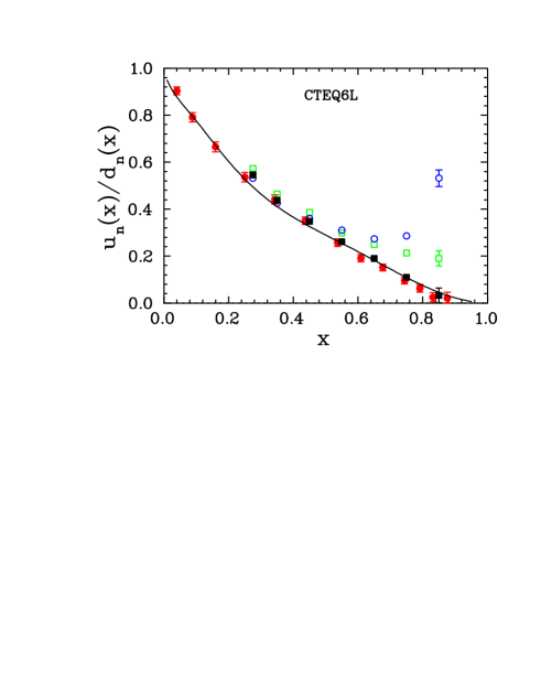
Figure 4: Ratio of u quarks to d quarks in the neutron from several analyses of deuteron and proton data. The solid line is the CTEQ6L parameterization

Taking what we have learned from the proton, we now consider the neutron. Figure 4 shows the ratio of the up- to down-quark distributions in the neutron, as extracted from various analyses of deuteron and proton data [31, 32, 33] (using different models for the nuclear corrections in dueterium), and from the CTEQ6L [26] parameterization. For $x\to 0$, the up and down quark distributions are similar, and the contribution to the charge distribution from this limit should be similar to that of the proton; a broad distribution of net positive charge. For $x=0.3$ and above, the $u$ quark distribution is less than half the $d$ quark distribution, yielding a net negative contribution to the charge. Because the distribution of quarks is more localized near $b=0$ as $x$ increases, a negative peak can be formed if there is a sufficiently large contribution from down quarks at large $x$ values. Above $x=0.5$, $d_{n}(x)/u_{n}(x)$ is at least three, except for the density-based extrapolation (blue circles), and continues to increase with $x$. As discussed in Ref. [33], even if one uses a density-based extrapolation of the EMC effect to apply nuclear corrections, the implementation used in this analysis significantly overestimates the effect for deuterium, and yields an unrealistically large result at very large $x$ values. In this region, the net impact on the charge distribution will be negative, and will be peaked at smaller values of $b$. This is shown in Fig. 5, which separately shows the contributions to the neutron charge density from $u$ and $d$ quarks based on the GPD of Ref. [22]. The distributions of Refs. [21, 23] yield somewhat different results, but exhibit the same qualitative behavior. For example, the GPDs of Ref. [22], shown in Fig. 5, yield a negative central neutron charge density for values of $x$ between 0.15 and 0.3 and between 0.3 and 0.465, but for the GPDs of Ref. [21], the central density is positive unless $x$ is slightly greater than 0.465.

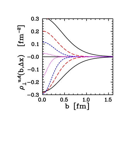
Figure 5: The $u$ and $d$ quark contributions to the neutron transverse charge density, $\rho_{\perp}^{u}(b,\Delta x)$ and $\rho_{\perp}^{d}(b,\Delta x)$. Here the quark flavor refers to the neutron ($u$ in the proton is $d$ in the neutron). The curves correspond to the same $\Delta x$ regions as in Fig. 3. The largest contributions come from small $x$, where $u$ and $d$ quarks contribute similar amounts of charge. As one goes to larger $x$ values, the charge is shifted to smaller values of $b$, while at the same time the up quark distribution drops rapidly with respect to the down quarks. Reprinted with permission from Ref. ⁶. Copyright 2008 by the American Physical Society.

Next we examine the total charge distribution of the neutron. Fig. 6 shows the charge distribution of the neutron, separating out the contributions from low and high $x$ regions, and shows $b\rho_{\perp}^{n}$ to suppress the very large density at the center. For $x<0.23$ the charge distribution (dotted line) is positive for $b<1.5$ fm and slightly negative distribution at larger radii. For $x>0.23$, the contribution (dashed line) is largely negative, and highly localized below 0.5 fm. The negative region at the center of the neutron transverse charge distribution arises a natural consequence of the model-independent definition of the charge density. The low momentum partons have a larger spatial extent and reproduce the intuitive result of the pion cloud picture: a positive core with a small negative tail at large distances, although the negative tail is difficult to see for this parameterization of the GPD, given the large scale required to show the negative core at small $b$.

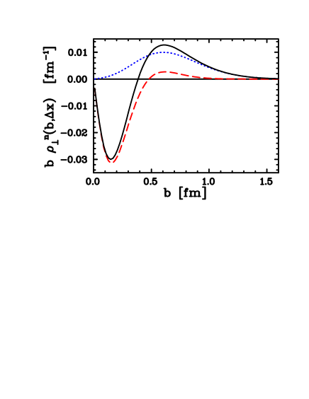
Figure 6: Transverse charge density for the neutron. The dotted line is the contribution from $x<0.23$, dashed is that for $x>0.23$, and the solid is the total. Reprinted with permission from Ref. ⁶. Copyright 2008 by the American Physical Society.

We also study the quantity

$$\rho_{\perp}(b,x)\equiv\sum_{q}\;e_{q}\rho^{q}_{\perp}(b,x)$$ (19)

to obtain a pictorial view of the transverse charge density for specific values of $x$ (Fig. 7). The striking feature of the negative spike appears prominently for $x=0.3$ and more prominently for $x=0.5$. These figures show how the central negative charge density appears more and more prominent as $x$ increases. Clearly the negatively charged $d$ quarks dominate at the center of the neutron.

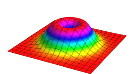
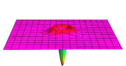
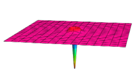
Figure 7: Neutron generalized parton distributions $\rho(b,x)$ for $x=0.1$ (top), $x=0.3$ (middle), and $x=0.5$ (bottom).

As discussed earlier, the longitudinal-momentum weighting used in determining the nucleon center of mass leads to a strong correlation between the position of the struck quark and the center of the nucleon for large $x$. It is informative to try and remove this effect to obtain something that is closer to our intuitive picture. We can do this by examining the position of the struck quark relative to the center of the spectator system, so that the struck quark does not influence the definition of the center of the neutron. This can be approximated by looking at the position of the struck quark relative to the spectators. We use Eq. (14) with the origin set to the center of momentum, for a struck quark at $(x_{1},{\bf b_{1}})\equiv(x,{\bf b})$, to determine the momentum-weighted spectator position, ${\bf b_{\rm spec}}$, and the relative distance from the struck quark to the spectator quarks:

$$x_{1}{\bf b}_{1}+\sum_{i>1}x_{i}{\bf b}_{i}=x{\bf b}+(1-x){\bf b}_{\rm spec}=0,$$ (20)

$${\bf B_{\rm rel}}={\bf b}-{\bf b_{\rm spec}}=\frac{{\bf b}}{(1-x)}=\bf{B_{\rm rel}}.$$ (21)

We exhibit the dependence on ${\bf B_{\rm rel}}$ by defining a function

$$\rho^{\rm Spec}_{\perp}({\bf B}_{rel},x)\equiv\rho_{\perp}({\bf B}_{rel}(1-x),x)$$ (22)

which gives the probability that a struck quark of longitudinal momentum fraction $x$ is a distance ${\bf B_{\rm rel}}$ away from the spectator center of momentum. Figure 8 shows this rescaled version of $\rho_{\perp}(b)$, with the contribution at each $x$ value normalized to unity at $b=0$. The quantity $\rho^{\rm Spec}_{\perp}({\bf B}_{\rm rel},x)$ does not correspond to a true density, but can provide a better approximation to our intuitive picture of the charge distribution, as it removes the influence of the struck quark on defining the center of the nucleon. While the charge distribution coming from very low $x$ quarks has a greater spatial extent, the decreasing width of the $\rho_{\perp}(b)$ distribution for large $x$ quarks is essentially completely removed when looking at $B_{\rm rel}$.

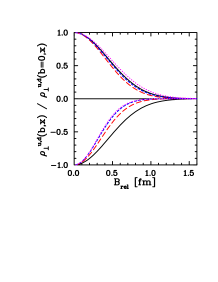
Figure 8: The $u$ and $d$ quark contributions to $\rho^{{\rm Spec},n}_{\perp}(B_{\rm rel},x)$ see Eq. (22). vs $B_{\rm rel}$ for $x=0.1$ (solid), 0.3 (long-dash), 0.5 (short-dash), and 0.7 (dotted). The curves are scaled to unity at $B_{\rm rel}=0$. Here the quark flavor refers to the neutron ($u$ in the proton is $d$ in the neutron). Reprinted with permission from Ref. ⁶. Copyright 2008 by the American Physical Society.

We summarize our findings with the statement that, using the model GPDs of Refs. [22, 21, 23], the dominance of the neutron’s $d$ quarks at high values of $x$ leads to a negative contribution to the charge density which, due to the definition of ${\bf b}$, becomes localized near the center of mass of the neutron. This localization does not appear when examined as a function of the position of the struck quark relative to the spectators, and is an consequence of the fact that quarks with a large longitudinal momentum play an important role in defining the transverse position of the neutron.

References

- [1] H. Gao, Int. J. Mod. Phys. E 12 (2003) 1 [Erratum-ibid. E 12 (2003) 567].
- [2] C. E. Hyde-Wright and K. de Jager, Ann. Rev. Nucl. Part. Sci. 54, (2004) 21.
- [3] C. F. Perdrisat, V. Punjabi and M. Vanderhaeghen, Prog. Part. Nucl. Phys. 59 (2007) 694.
- [4] J. Arrington, C. D. Roberts and J. M. Zanotti, J. Phys. G 34 (2007) S23
- [5] G. A. Miller, Phys. Rev. Lett. 99 (2007) 112001.
- [6] G. A. Miller and J. Arrington, Phys. Rev. C 78 (2008) 032201.
- [7] D.E. Soper, Phys. Rev. D 5 (1972) 1956; J. Kogut and D.E. Soper, Phys. Rev. D 1 (1970) 2901.
- [8] D. E. Soper, Phys. Rev. D 15 (1977) 1141.
- [9] M. Burkardt, Int. J. Mod. Phys. A 18 (2003) 173.
- [10] M. Diehl, Eur. Phys. J. C 25 (2002)223, [Erratum-ibid. C 31 (2003) 277].
- [11] G. A. Miller, E. Piasetzky and G. Ron, Phys. Rev. Lett. 101 (2008) 082002.
- [12] C. E. Carlson and M. Vanderhaeghen, Phys. Rev. Lett. 100, 032004 (2008)
- [13] R. Bradford, A. Bodek, H. Budd and J. Arrington, Nucl. Phys. Proc. Suppl. 159 (2006) 127
- [14] J. J. Kelly, Phys. Rev. C 70 (2004) 068202.
- [15] J. Arrington, Phys. Rev. C 69, 022201 (R) (2004);
- [16] A. W. Thomas, S. Théberge and G. A. Miller, Phys. Rev. D 24 (1981) 216; G. A. Miller, Phys. Rev. C 66 (2002) 032201.
- [17] J. L. Friar, Part. Nucl. 4, 153 (1972); R. D. Carlitz, S. D. Ellis and R. Savit, Phys. Lett. B 68, 443 (1977); N. Isgur, G. Karl and D. W. L. Sprung, Phys. Rev. D 23, 163 (1981).
- [18] X. D. Ji, Phys. Rev. D 55 (1997) 7114
- [19] A. V. Radyushkin, Phys. Rev. D 56 (1997) 5524
- [20] M. Burkardt, Phys. Rev. D 62 (2000) 071503 [Erratum-ibid. D 66 (2002) 119903]
- [21] M. Guidal, M. V. Polyakov, A. V. Radyushkin and M. Vanderhaeghen, Phys. Rev. D 72 (2005) 054013
- [22] M. Diehl, T. Feldmann, R. Jakob and P. Kroll, Eur. Phys. J. C 39, 1 (2005)
- [23] S. Ahmad, H. Honkanen, S. Liuti and S. K. Taneja, Phys. Rev. D 75, 094003 (2007)
- [24] B. C. Tiburzi, W. Detmold and G. A. Miller, Phys. Rev. D 70, 093008 (2004)
- [25] S. D. Drell and T. M. Yan, Phys. Rev. Lett. 24, 181 (1970); G. B. West, Phys. Rev. Lett. 24, 1206 (1970).
- [26] J. Pumplin, D. R. Stump, J. Huston, H. L. Lai, P. M. Nadolsky and W. K. Tung, JHEP 0207, 012 (2002)
- [27] G. A. Miller, B. M. K. Nefkens and I. Slaus, Phys. Rept. 194, 1 (1990).
- [28] G. A. Miller, Phys. Rev. C 57, 1492 (1998)
- [29] J. T. Londergan and A. W. Thomas, Prog. Part. Nucl. Phys. 41, 49 (1998)
- [30] G. A. Miller, A. K. Opper and E. J. Stephenson, Ann. Rev. Nucl. Part. Sci. 56, 253 (2006)
- [31] L. W. Whitlow, E. M. Riordan, S. Dasu, S. Rock and A. Bodek, Phys. Lett. B 282, 475 (1992).
- [32] W. Melnitchouk and A. W. Thomas, Phys. Lett. B 377, 11 (1996)
- [33] J. Arrington, F. Coester, R. J. Holt and T. S. Lee, J. Phys. G 36, 025005 (2009)