Numerical reconstruction of photon-number statistics from photocounting statistics:
Regularization of an ill-posed problem

Abstract

We demonstrate a practical possibility of loss compensation in measured photocounting statistics in the presence of dark counts and background radiation noise. It is shown that satisfactory results are obtained even in the case of low detection efficiency and large experimental errors.

Photoelectric detection of quantum light PhotoDetection ; MandelBook is a basic experimental technique in a variety of fundamental and applied investigations. In principle, the photon-number resolved detectors enable one to determine the number of photons in radiation fields. In practice, the number of photocounts may significantly differ from the number of photons due to losses, dark counts, and background radiation. The modern technologies enable one to get the detection efficiency near 0.9 and even more Waks . However, such an improvement leads, as rule, to an increase in the dark count rate Takeuchi . Furthermore, different losses occur at all the stages of generation, manipulation, and transmission of quantum light.

The effects of losses and noise in photocounting statistics can be compensated in two different ways. First, the active compensation can be realized by using the homodyne detection and preamplification of the signal by a degenerate parametric amplifier Leonhardt . Another possibility is a numerical manipulation with the measured data – the corresponding technique of loss compensation has been discussed in Ref. Kiss . The problem is that the corresponding series can diverge for small efficiency $\eta$ in many important cases that require application of a special technique of the analytical continuation Herzog .

However, the most serious problem is that the method of numerical compensation occurs to be unstable with respect to small experimental inaccuracies. Small experimental errors in photocounting statistics may lead to large errors in the reconstructed photon-number statistics even for large detection efficiencies. This problem should be resolved by application of special regularization methods. For example, the photon-number statistics of a laser radiation has been reconstructed by the method of maximum entropy in Ref. Lee . The least-squares regularization technique for loss compensation in photocounting statistics has been recently considered in the context of the tomography of the quantum detectors Lundeen . The numerical compensation of losses in multi-pixel detectors has been discussed in Afek . The method of maximum-likelihood estimation demonstrates satisfactory results for quantum-state reconstruction in the presence of losses Mogilevtsev and, consequently, it can be applied for loss compensation in photocounting statistics. An alternative technique of the regularization, which requires measurements with different values of the efficiency, has been proposed in Ref. Zambra .

In the present contribution we reexamine the method of numerical compensation of losses. We demonstrate that the regularization of the corresponding ill-posed problem (see, e.g., Tikhonov and Morozov ) enables one to apply this technique even for low values of the efficiency $\eta$. Moreover, our consideration includes numerical compensation of dark counts and effects of background radiation. Besides, the method demonstrates satisfactory results under a realistic assumption that the efficiency and the noise-counts rate are known with a certain inaccuracy. We demonstrate that the proposed technique can be applied for different photocounting statistics including highly-nonclassical cases.

Let us start with consideration of a single-mode quantum light characterized by the density operator $\hat{\varrho}$. If $\hat{n}$ is the corresponding photon-number operator and $\left|n\right\rangle$ is its eigenvector, the photon-number distribution is given by PhotoDetection ; MandelBook

$$p_{n}=\left\langle n\left|\hat{\varrho}\right|n\right\rangle=\mathop{\mathrm{Tr}}\nolimits\left(:\frac{\hat{n}^{n}}{n!}\,\exp\left(-\hat{n}\right):\,\hat{\varrho}\right).$$ (1)

In the presence of losses, dark counts, and background radiation it differs from the photocounting distribution Karp ; Semenov ,

$$\mathcal{P}_{n}=\mathop{\mathrm{Tr}}\nolimits\left(:\frac{\left(\eta\,\hat{n}\,+N_{\mathrm{nc}}\right)^{n}}{n!}\,\exp\left(-\eta\,\hat{n}-N_{\mathrm{nc}}\right):\,\hat{\varrho}\right),$$ (2)

where $\eta$ and $N_{\mathrm{nc}}$ are the efficiency and the mean number of noise counts, respectively. The aim of this work is to develop a mathematical technique for reconstruction of the photon-number distribution $p_{n}$ from the experimentally-measured photocounting distribution $\mathcal{P}_{n}$.

The photocounting distribution $\mathcal{P}_{n}$ is expressed in terms of the photon-number distribution $p_{n}$ as (see Semenov ; Lee )

$$\mathcal{P}_{m}=\sum\limits_{n=0}^{+\infty}S_{m|n}\left(\eta,N_{\mathrm{nc}}\right)\,p_{n}.$$ (3)

Here,

$$S_{m|n}\left(\eta,N_{\mathrm{nc}}\right)=e^{-N_{\mathrm{nc}}}N_{\mathrm{nc}}^{m-n}\eta^{n}\frac{n!}{m!}\mathop{\mathrm{L}}\nolimits_{n}^{m-n}\!\left(\frac{N_{\mathrm{nc}}(\eta-1)}{\eta}\right)$$ (4)

for $m\geq n$ and

$$S_{m|n}\left(\eta,N_{\mathrm{nc}}\right)=e^{-N_{\mathrm{nc}}}(1-\eta)^{n-m}\eta^{m}\mathop{\mathrm{L}}\nolimits_{m}^{n-m}\!\left(\frac{N_{\mathrm{nc}}(\eta-1)}{\eta}\right)$$ (5)

for $m\leq n$ are the probabilities to get $m$ photocounts under the condition that $n$ photons are present. $\mathop{\mathrm{L}}\nolimits_{n}^{m}\!\left(x\right)$ is the Laguerre polynomial. Expression (3) is formally inverted as

$$p_{n}=\sum\limits_{m=0}^{+\infty}S_{n|m}^{-1}\left(\eta,N_{\mathrm{nc}}\right)\,\mathcal{P}_{m},$$ (6)

where

$$S_{n|m}^{-1}\left(\eta,N_{\mathrm{nc}}\right)=\frac{1}{\eta^{n}}\Phi\left(n+1,n-m+1;\frac{N_{\mathrm{nc}}(1-\eta)}{\eta}\right)$$

$$\times e^{N_{\mathrm{nc}}}\frac{(-N_{\mathrm{nc}})^{n-m}}{(n-m)!}$$ (7)

for $m\leq n$ and

$$S_{n|m}^{-1}\left(\eta,N_{\mathrm{nc}}\right)=e^{N_{\mathrm{nc}}}\Phi\left(m+1,m-n+1;\frac{N_{\mathrm{nc}}(1-\eta)}{\eta}\right)$$

$$\times{m\choose n}\frac{1}{\eta^{n}}\left(1-\frac{1}{\eta}\right)^{m-n}$$ (8)

for $m\geq n$ is the matrix inverse to $S_{m|n}\left(\eta,N_{\mathrm{nc}}\right)$. $\Phi\left(n,m;x\right)$ is the Kummer hypergeometric function.

As mentioned, expression (6) as the solution of Eq. (3) is unstable with respect to small experimental inaccuracies of $P_{n}$. Moreover, similar to the case of zero noise counts Kiss ; Herzog , this series diverges in many important cases. Hence, Eqs. (6)–(8) cannot be applied in the general case. This fact is a consequence of a more general statement that Eq. (3) is an ill-posed problem Tikhonov . Such a problem can be treated by using the appropriated regularization methods Tikhonov ; Morozov ; Engl .

A priori information, such as numbers at which photon-number and photocounting distributions can be truncated Welsch , is used in the regularization of the ill-posed problem. In addition, the basic properties of the photon-number distribution,

$$p_{n}\geq 0,$$ (9)

$$\sum\limits_{n}p_{n}=1,$$ (10)

are applied in the considered case. Other a priori information can also be useful for the regularization of the ill-posed problem depending on a given physical situation.

In different problems of quantum optics the least-squares inversion and the Tikhonov regularization lead to satisfactory results (for a review see, e.g., Welsch ). In this contribution, we apply the Landweber algorithm Landweber adopted to the regularization of similar problems Engl – a technique, which demonstrates a good computer compatibility Brodyn . The projected Landweber algorithm Byrne is the iteration process,

$$p^{(j)}=\Pi_{C}\left[p^{(j-1)}+\chi\left(S^{\dagger}\,\mathcal{P}-S^{\dagger}S\,p^{(j-1)}\right)\right],$$ (11)

where $p^{(j)}=\left\{p_{n}^{(j)}\right\}$ is the $j\textrm{th}$ iteration for the photon-number distribution, $\mathcal{P}=\left\{\mathcal{P}_{m}\right\}$, $S=\left\{S_{m|n}\right\}$, and $\chi$ is the relaxation parameter. $\Pi_{C}$ is the projector on the closed convex set $C$ defined by Eq. (9) and, in special cases, by other additional conditions. Condition (10) can be used to track the accuracy of the obtained results. The starting values are usually chosen as $p_{n}^{(0)}=0$.

To illustrate the method let us give some numerical simulations. We start from the thermal state,

$$\hat{\varrho}=\frac{1}{1+\bar{n}_{\mathrm{th}}}\left(\frac{\bar{n}_{\mathrm{th}}}{1+\bar{n}_{\mathrm{th}}}\right)^{\hat{n}}$$ (12)

with $\bar{n}_{\mathrm{th}}=30$, and derive from Eq. (2) the photocounting distribution $\mathcal{P}_{n}$ for $\eta=0.34$ and $N_{\mathrm{nc}}=0.30$. The measured data are simulated with $\nu=5\times 10^{4}$ sampling events. The corresponding relative error (in terms of the Euclidian norm) is $\delta_{P}=0.03$. The simulated data are then used as an input of Landweber algorithm (11) for the reconstruction of the photon-number distribution with inaccurate values of the efficiency $\tilde{\eta}=0.35$ and the mean number of noise counts $\tilde{N}_{\mathrm{nc}}=0.29$. The result of this procedure (see Fig. 1) is in a reasonable agreement with the initially chosen photon-number distribution, the relative error is $\delta_{p}=0.05$, and the relative residual is $\tilde{\delta}_{p}=0.019$. It is worth noting that in the given example series (3) diverges even in the absence of experimental errors Kiss . Nevertheless, algorithm (11) demonstrates high efficiency for the considered case.

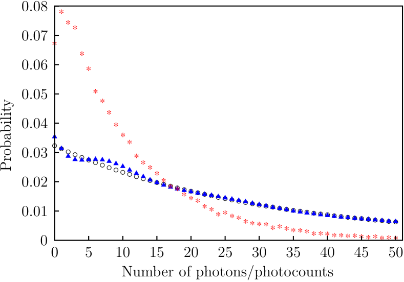
Figure 1: (Color online) The photon-number, $p_{n}$, and photocounting, $\mathcal{P}_{n}$, distributions of the thermal state, $\bar{n}_{\mathrm{th}}=30$. The circles and triangles are the initially chosen and reconstructed ($\tilde{\eta}=0.35$, $\tilde{N}_{\mathrm{nc}}=0.29$) photon-number distributions, respectively. The asterisks show the simulated photocounting distribution ($\nu=5\times 10^{4}$, $\eta=0.34$, $N_{\mathrm{nc}}=0.30$).

Another example is the single-photon-added thermal state (SPATS),

$$\hat{\varrho}=\frac{\hat{n}}{\bar{n}_{\mathrm{th}}\left(1+\bar{n}_{\mathrm{th}}\right)}\left(\frac{\bar{n}_{\mathrm{th}}}{1+\bar{n}_{\mathrm{th}}}\right)^{\hat{n}}$$ (13)

with $\bar{n}_{\mathrm{th}}=10$. Such a state has been recently realized experimentally and its nonclassical properties have been verified SPATS . The numerical simulation is performed for $\nu=5\times 10^{3}$, $\eta=0.7764$, and $N_{\mathrm{nc}}=0.748$, with the relative error $\delta_{P}=0.025$. The photon-number distribution (reconstructed with $\tilde{\eta}=0.77$, $\tilde{N}_{\mathrm{nc}}=0.75$) is shown in Fig. 2. The relative error is $\delta_{p}=0.041$ and the relative residual is $\tilde{\delta}_{p}=0.020$. In this example series (6) formally converges. However, attempts to apply this series for the direct reconstruction of $p_{n}$ result in the large noise effects caused by small experimental inaccuracies even for sufficiently large number of sampling events ($\nu=5\times 10^{5}$, $\delta_{P}=0.0079$) and exact values of $\eta$ and $N_{\mathrm{nc}}$ (see Fig. 3).

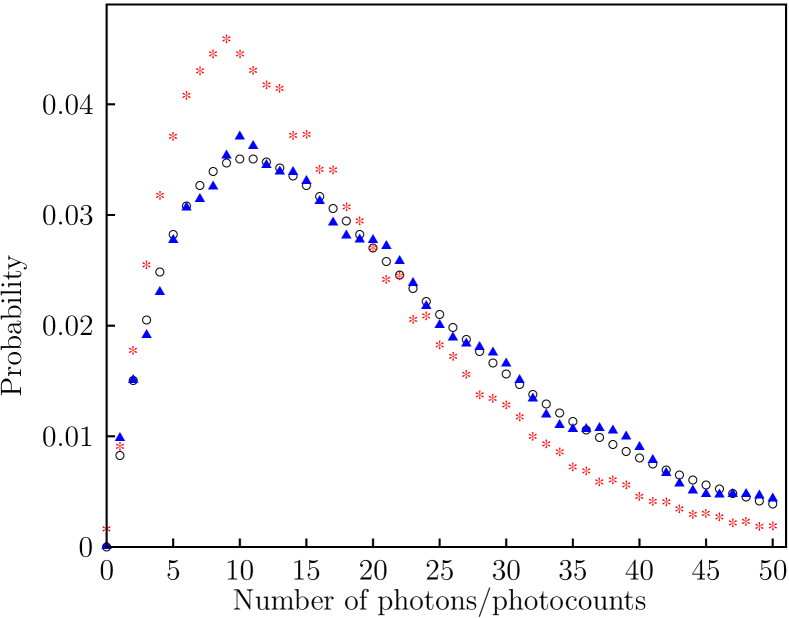
Figure 2: (Color online) The photon-number, $p_{n}$, and photocounting, $\mathcal{P}_{n}$, distributions of the SPATS, $\bar{n}_{\mathrm{th}}=10$. The circles and triangles are the initially chosen and reconstructed ($\tilde{\eta}=0.77$, $\tilde{N}_{\mathrm{nc}}=0.75$) photon-number distributions, respectively. The asterisks show the simulated photocounting distribution ($\nu=5\times 10^{3}$, $\eta=0.7764$, $N_{\mathrm{nc}}=0.748$).

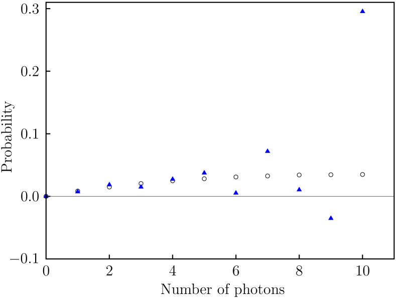
Figure 3: (Color online) The photon-number distribution, $p_{n}$, of the SPATS, $\bar{n}_{\mathrm{th}}=10$. The circles and triangles are the initially chosen and reconstructed ($\nu=5\times 10^{5}$, $\eta=0.7764$, ${N}_{\mathrm{nc}}=0.748$) distributions in Eq. (6), respectively. The result of such a reconstruction demonstrates much stronger noise effect in comparison with the Landweber algorithm (see Fig. 2).

Algorithm (11) demonstrates a reasonable agreement with the initially chosen photocounting distribution even in the case of rather large error in the simulated data. To illustrate this fact, we consider the superposition of the coherent states,

$$\left|\psi\right\rangle=\frac{1}{\sqrt{2\left(1+e^{-2\left|\alpha\right|^{2}}\right)}}\Big{(}\left|\alpha\right\rangle+\left|-\alpha\right\rangle\Big{)},$$ (14)

$\left|\alpha\right|^{2}=23.9$. The initial data are simulated with $\nu=5\times 10^{3}$, $\eta=0.613749$, and $N_{\mathrm{nc}}=1.763442$. The relative error is $\delta_{P}=0.098$. The photon-number distribution is reconstructed for $\tilde{\eta}=0.59$, $\tilde{N}_{\mathrm{nc}}=1.77$ (see Fig. 4). The relative error of the reconstructed distribution, $\delta_{p}=0.125$, and the relative residual, $\tilde{\delta}_{p}=0.051$, are of the same order as for the initially simulated data. It should be stressed that for the state (14) $p_{n}\neq 0$ only for even photon numbers $n$. This a priori information is used in the projector $\Pi_{C}$, [cf. Eq. (11)].

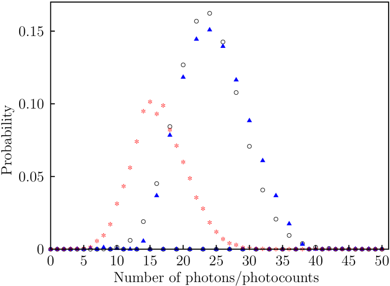
Figure 4: (Color online) The photon-number, $p_{n}$, and photocounting, $\mathcal{P}_{n}$, distributions of the superposition of the coherent states $\left|\alpha\right|^{2}=23.9$. The circles and triangles are the initially chosen and reconstructed ( $\tilde{\eta}=0.59$, $\tilde{N}_{\mathrm{nc}}=1.77$) photon-number distributions, respectively. The asterisks show the simulated photocounting distribution ($\nu=5\times 10^{3}$, $\eta=0.613749$, $N_{\mathrm{nc}}=1.763442$).

In conclusion, we have obtained the expression for photocounting distribution in terms of the photon-number distribution. However, the inverted expression cannot be used in the most practical situations – it is unstable with respect to small experimental inaccuracies and the corresponding series can diverge. At the same time, the regularization of this ill-posed problem by the Landweber algorithm enables one to compensate losses and noise counts even for low efficiencies, high noise-counts rates, and inaccurate knowledge of their values.

- (1) L. Mandel, E.C.G. Sudarshan, and E. Wolf, Proc. Phys. Soc. (London) 84, 435 (1964); R.J. Glauber, Phys. Rev. 130, 2529 (1963) 131, 2766 (1963); R.J. Glauber, Phys. Rev. 131, 2766 (1963); P. L. Kelley and W. H. Kleiner, Phys. Rev. 136, 316 (1964).
- (2) L. Mandel and E. Wolf, Optical Coherence and Quantum Optics (Cambridge University Press, 1995).
- (3) E. Waks, E. Diamanti, B.C. Sanders, S. D. Bartlett, and Y. Yamamoto, Phys. Rev. Lett. 92, 113602 (2004).
- (4) S. Takeuchi, J. Kim, Y. Yamamoto, and H. H. Hogue, Appl. Phys. Lett. 74, 1063 (1999).
- (5) U. Leonhardt and H. Paul, Phys. Rev. Lett. 72, 4086 (1994); Progr. Quantum Electron. 19, 89 (1995).
- (6) T. Kiss, U. Herzog, and U. Leonhardt, Phys. Rev. A 52, 2433 (1995).
- (7) U. Herzog, Phys. Rev. A 53, 1245 (1996).
- (8) H. Lee, U. Yurtsever, P. Kok, G. M. Hockney, C. Adami, S. L. Braunstein, and J. P. Dowling, J. Mod. Opt. 51, 1517 (2004).
- (9) J. S. Lundeen et al., Nature Physics 5, 27 (2009).
- (10) I. Afek, A. Natan, O. Ambar, and Y. Silberberg, Phys. Rev. A 79, 043830 (2009).
- (11) Z. Hradil, D. Mogilevtsev, and J. Řeháček, Phys. Rev. Lett. 96, 230401 (2006).
- (12) G. Zambra and M. G. A. Paris, Phys. Rev. A 74, 063830 (2006).
- (13) A. N. Tikhonov and V. Y. Arsenin, Solutions of Ill-Posed Problems (W.H. Winston & Sons, NY, 1977).
- (14) V. A. Morozov, Regularization Methods for Ill-Posed Problems (CRC Press, Florida, 1993).
- (15) S. Karp, E. L. O’Neill, and R. M. Gagliardi, Proc. IEEE 58, 1611 (1970).
- (16) A. A. Semenov, A. V. Turchin, and H. V. Gomonay, Phys. Rev. A 78, 055803 (2008); 79, 019902(E) (2009).
- (17) H. W. Engl, M. Hanke, and A. Neubauer, Regularization of Inverse Problems (Kluwer, Dordrecht, 1996).
- (18) D.-G. Welsch, W. Vogel, and T. Opartný, Progr. Opt. 39, 63 (1999).
- (19) L. Landweber, Amer. J. Math. 73, 615 (1951).
- (20) M. S. Brodyn and V. N. Starkov, Quantum Electron. 37, 679 (2007).
- (21) C. Byrne, Inverse Problems 20, 103 (2004); M. Bertero and P. Boccacci, Introduction to Inverse Problem in Imaging (IOP Publishing, Bristol, 1998).
- (22) A. Zavatta, V. Parigi, and M. Bellini, Phys. Rev. A 75, 052106 (2007); T. Kiesel, W. Vogel, V. Parigi, A. Zavatta, and M. Bellini, Phys. Rev. A 78, 021804(R) (2008).