Interfacing nuclear spins in quantum dots to cavity or traveling-wave fields

Abstract

We show how to realize a quantum interface between optical fields and the polarized nuclear spins in a singly charged quantum dot, which is strongly coupled to a high-finesse optical cavity. An effective direct coupling between cavity and nuclear spins is obtained by adiabatically eliminating the (far detuned) excitonic and electronic states.
The requirements needed to map qubit and continuous variable states of cavity or traveling-wave fields to the collective nuclear spin are investigated: For cavity fields, we consider adiabatic passage processes to transfer the states. It is seen that a significant improvement in cavity lifetimes beyond present-day technology would be required for a quantum interface. We then turn to a scheme which couples the nuclei to the output field of the cavity and can tolerate significantly shorter cavity lifetimes. We show that the lifetimes reported in the literature and the recently achieved nuclear polarization of $\sim 90$% allow both high-fidelity read-out and write-in of quantum information between the nuclear spins and the output field.
We discuss the performance of the scheme and provide a convenient description of the dipolar dynamics of the nuclei for highly polarized spins, demonstrating that this process does not affect the performance of our protocol.

1 Introduction

An important milestone on the path to quantum computation and quantum communication networks is the coupling of “stationary” qubits for storage and data processing (usually assumed to be realized by material systems such as atoms or electrons) and mobile “flying” qubits for communication (typically photons) [1, 2]. Detection and subsequent storage of information is inapplicable in quantum information as an unknown quantum state cannot be determined faithfully by a measurement. Hence the development of “light-matter interfaces” that allow the coherent write-in and read-out of quantum information has been the subject of intense theoretical research [3, 4, 5]. Two paths have been identified to make light efficiently couple to a single atomic quantum system: the use of a high-finesse cavity coupled to a single atom or the use of an optically thick ensemble of atoms, in whose collective state the quantum information is to be stored. Both have resulted in the experimental demonstration of such interfaces [6, 7, 8, 9, 10]. Even without strong coupling a quantum interface can be realized by combining the probabilistic creation of entanglement between atom and light with teleportation. This approach has been demonstrated with trapped ions [11].

For qubits realized by electron spins in quantum dots [12, 13] such interfaces have yet to be realized, though in particular for self-assembled quantum dots [14], which have many atom-like properties, several proposals exist to map photonic states to an electron in a quantum dot [13, 15] in analogy to the atomic schemes. Strong coherent coupling between a single quantum system and a single mode of high-Q micro- and nano-cavities has been demonstrated experimentally [16, 17, 18, 19], raising the prospect of coupling light to the quantum dot’s electronic state by adapting protocols such as [3].

Despite their good isolation from many environmental degrees of freedom, the electron-spin coherence time in today’s quantum dots is limited mainly due to strong hyperfine coupling to lattice nuclear spins. Moreover, the capacity of such an interface is one qubit only, making the interfacing difficult for many-photon states of the light field as used in continuous variable quantum information processing. In contrast, the ensemble of lattice nuclear spins could provide a high-dimensional and long-lived quantum memory [20].

We show in the following how to couple an optical field directly to the nuclear spin ensemble, thus interfacing light to an exceptionally long-lived mesoscopic system that enables the storage and retrieval of higher-dimensional states and is amenable to coherent manipulation via the electron spin [21]. The system we consider is a charged quantum dot strongly coupled to a high-finesse optical cavity by a detuned Raman process, introduced in Section 2. In Section 3 we show that by adiabatically eliminating the trion and the electron spin different effective couplings (that can be tuned on- and off-resonant) between light and nuclear spins are achieved. In Sections 4 and 5, we demonstrate that the state of the cavity field can be directly mapped to the nuclear spins using the methods of Landau-Zener transitions [22, 23] and stimulated Raman adiabatic passage (STIRAP) [24], respectively, where the latter yields a reduction of the time required for write-in. However, the drawback of this approach is that it requires very long cavity lifetimes. To address this problem we discuss in Section 6 at length an approach that was proposed in [25] (here, we discuss it for an experimentally more promising setup), which is robust against cavity decay: the read-out maps the nuclear state to the output mode of the cavity, while the write-in proceeds by deterministic creation of entanglement between the nuclear spins and the cavity output-mode and subsequent teleportation [26]. In Section 6, we give further insight into this system and its dynamics: we describe the full time evolution of the system, compute the read-out fidelity and derive the shape of the output mode-function. Moreover, we show that apart from mapping light states to the nuclear spins, the interaction we describe can be used to generate an arbitrary Gaussian state. In Section 7 we discuss different aspects concerning the experimental realization and the approximations used in our scheme such as the internal nuclear dynamics, dominated by dipolar interactions, which we model numerically and corrections to the first order bosonic description.

2 The system

We consider a self-assembled III-V quantum dot (QD) with a single conduction-band electron strongly coupled to a high-Q nano-cavity [see figure 1a)]. At zero magnetic field, the two electronic ground states $\left|\pm 1/2\right>$ (s-type conduction band states) are degenerate and the only dipole allowed transitions are to the trion states $\left|\pm 3/2\right>$ with spin $+3/2$ and spin $-3/2$ (heavy-hole valence band state) with $\sigma^{\pm}$ polarized light. An external magnetic field $B_{z}$ in $z$-direction, perpendicular to the growth ($y$-) direction, Zeeman splits the two electronic states and the trion states and leads to eigenstates $\left|\pm\right>=\frac{1}{\sqrt{2}}(\left|1/2\right>\pm i\left|-1/2\right>)$ and $\left|T_{\pm}\right>=\frac{1}{\sqrt{2}}(\left|3/2\right>\pm i\left|-3/2\right>)$. The states $\left|+\right>\Leftrightarrow\left|T_{+}\right>$ and $\left|-\right>\Leftrightarrow\left|T_{-}\right>$ can be coupled [see figure 1b)] by horizontally polarized light, and $\left|+\right>\Leftrightarrow\left|T_{-}\right>$ and $\left|-\right>\Leftrightarrow\left|T_{+}\right>$ by vertically polarized light:

$$H_{\mathrm{opt}}= \frac{\Omega_{c}}{2}\,(a^{\dagger}\left|-\right>\left<T_{+}\right|+a^{\dagger}\left|+\right>\left<T_{-}\right|+\mathrm{h.c.})$$ (1)

$$+\frac{\Omega_{l}}{2}\,(e^{+i\omega_{l}t}(\left|+\right>\left<T_{+}\right|+\left|-\right>\left<T_{-}\right|)+\mathrm{h.c.})$$

$$+\omega_{c}\,a^{\dagger}a+\omega_{T_{+}}\left|T_{+}\right>\left<T_{+}\right|+\omega_{T_{-}}\left|T_{-}\right>\left<T_{-}\right|+\omega_{e}S^{z}.$$

Here, $\hbar=1$, $S^{z}$ is the electron spin operator, $a^{\dagger}$ and $a$ are creation and annihilation operators of the single mode cavity field and $\omega_{c}$, $\omega_{l}$ denote the cavity and the laser frequency (which are vertically/horizontally polarized respectively) and $\Omega_{c}$, $\Omega_{l}$ the Rabi frequencies of the cavity and the laser field, respectively. The energies of the trion states $\left|T_{+}\right>$, $\left|T_{-}\right>$ are $\omega_{T_{+}}=\omega_{T}+\omega_{h}/2$ and $\omega_{T_{-}}=\omega_{T}-\omega_{h}/2$ where $\omega_{T}$ is the energy of the trion (without magnetic field), $\omega_{h}$ the energy of the hole Zeeman splitting and $\omega_{e}=g_{e}\,\mu_{b}B_{y}$ denotes the Zeeman splitting of the electronic states. The first term of the Hamiltonian given by (1) describes the coupling to the cavity field and the second term the coupling to a classical laser field. We assume both cavity decay and spontaneous emission rate of the QD to be much smaller than $\Omega_{c}$ and omit both processes in (1). Besides the coupling to optical fields, the electron spin in a QD also has a strong hyperfine interaction with the lattice nuclear spins, which is for s-type electrons dominated by the Fermi contact term

$$H_{\mathrm{hf}}=\frac{A}{2}(A^{+}S^{-}+S^{+}A^{-})+AS^{z}A^{z},$$ (2)

where $S^{\pm,z}$ are the electron spin operators and $A^{\pm,z}=\sum_{j}\,\alpha_{j}I_{j}^{\pm,z}$ are the collective nuclear spin operators (in a typical GaAs quantum dot, the number of

Figure 1: (a) A singly charged QD coupled to a high-Q optical cavity. (b) Level scheme of the QD. Optical and hyperfine driven transitions.

Ga and As nuclei lies between $N\sim 10^{4}$-$10^{6}$). The individual coupling constants $\alpha_{j}$ are proportional to the electron wave function at site $j$ (and the magnetic dipole moment of the $j$th nucleus) [27] and are normalized to $\sum_{j}\alpha_{j}=1$. The requirement for using nuclear spins as a quantum memory is to initialize them in a well-defined, highly polarized state. By this we mean that $\left<A^{z}\right>$ is close to its minimum value $\left<A^{z}\right>_{\mathrm{min}}$ ($\approx-1/2$ for spin-1/2 nuclei) and define the polarization as $P=\left<A^{z}\right>/\left<A^{z}\right>_{\mathrm{min}}$. Due to their small magnetic moments, nuclear spins are almost fully mixed even at dilution-fridge temperatures and fields of several Tesla. Over the past years, large progress in dynamical polarization experiments [28, 29, 30, 31] has been reported with nuclear polarization up to $60\%$, recently, nuclear polarization $>80$% has been achieved [32].

A convenient and intuitive description of the highly polarized nuclei with homogeneous coupling to the electron is provided by the Holstein Primakoff transformation [33], by which collective nuclear spin operators $A^{\pm,z}$ can be mapped to the bosonic operators $b$,$b^{\dagger}$, associating $A^{-}\rightarrow\frac{1}{\sqrt{N}}\sqrt{1-\frac{b^{\dagger}b}{N}}\,b$ and $A^{z}\rightarrow\frac{1}{N}\left(b^{\dagger}b-\frac{N}{2}\right)$. Assuming high polarization, the electron spin couples to a bosonic “spin wave” described by $A^{-}=\frac{1}{\sqrt{N}}b$ and $A^{z}=\frac{1}{N}(b^{\dagger}b-N/2)$ by a Jaynes-Cummings-like interaction

$$H_{\mathrm{hf}} = \frac{g_{n}}{2}(b^{\dagger}S^{-}+S^{+}b)+\frac{g_{n}}{\sqrt{N}}S^{z}\left(b^{\dagger}b-\frac{N}{2}\right),$$ (3)

with $g_{n}=A/\sqrt{N}$. The initial state of the nuclear spins is represented by a collection of bosonic modes, with $b$ in the vacuum state. One can generalize this description to the case of inhomogeneous coupling to the electron ($g_{n}=A\sqrt{\sum_{i}\alpha_{i}^{2}}$) and obtains an identical description in $0$th order in $\left<\frac{b^{\dagger}b}{N}\right>=(1-P)/2$ [34]. Corrections to this description arising from inhomogeneous coupling and not fully polarized nuclear spins will be discussed briefly in Section 7.2 and a detailed discussion can be found in [35]. It should be noted that the scheme we present does not require the bosonic description and could also be discussed directly in terms of the collective spin operators. The Fock basis would be replaced by $(A^{+})^{n}\left|\downarrow\dots\downarrow\right>$ and errors due to the inhomogeneity would have to be treated along the lines of [20] and [25]. The bosonic picture, however, allows a much more transparent treatment of the corrections to the ideal case, emphasizes the relation to quantum optical schemes, and gives access to the Gaussian toolbox of entanglement criteria and transformations.

3 Effective coupling between nuclei and cavity

Our aim is to obtain from $H=H_{\mathrm{opt}}+H_{\mathrm{hf}}$ a direct coupling between nuclear spins and light. The Hamiltonian $H$ describes a complicated coupled dynamics of cavity, nuclei and quantum dot. Instead of making use of the full Hamiltonian (and deriving the desired mapping, e.g., in the framework of optimal control theory) we aim for a simpler, more transparent approach. Closely following [25], we adiabatically eliminate [36] the trion and the electronic spin degree of freedom, which leads to a Hamiltonian $H_{\mathrm{el}}$ that describes a direct coupling between nuclear spins and light. As explained later, this can be achieved if the couplings (the Rabi frequency of the laser/cavity, the hyperfine coupling, respectively) are much weaker than the detunings to the corresponding transition:

$$\Delta^{\prime}_{T_{\pm}}\gg\Omega_{l},\Omega_{c}\sqrt{n},$$ (4a)

$$\sqrt{\Delta^{\prime}_{T_{\pm}}\,\,\tilde{\omega}_{e}}\gg\Omega_{l},\Omega_{c}\sqrt{n},$$ (4b)

$$\tilde{\omega}_{e}\gg g_{n}\sqrt{m}.$$ (4c)

Here, $\Delta^{\prime}_{T_{\pm}}=\omega_{T}-\omega_{l}\pm\omega_{h}/2+\tilde{\omega}_{e}/2=\Delta^{\prime}\pm\omega_{h}/2+\tilde{\omega}_{e}/2$ with $\Delta^{\prime}=\omega_{T}-\omega_{l}$, $n$ is the number of cavity photons and $m$ the number of nuclear excitations. Note that typically $\tilde{\omega}_{e}<\Delta^{\prime}_{T_{\pm}}$ such that condition (4a) becomes redundant. In addition to (4a)-(4c), we choose the adjustable parameters such that all first order and second order processes described by $H$ are off-resonant, but the (third order) process in which a photon is scattered from the laser into the cavity while a nuclear spin is flipped down (and its converse) is resonant. This leads to the desired effective interaction.

The idea of adiabatic elimination is to perturbatively approximate a given Hamiltonian by removing a subspace from the description that is populated only with a very low probability due to chosen initial conditions and detunings or fast decay processes. If initially unpopulated states (in our case the trion state $\left|X\right>$ and the electronic spin-up state $\left|\uparrow\right>$) are only weakly coupled to the initially occupied states, they remain essentially unpopulated during the time evolution of the system and can be eliminated from the description. The higher order transitions via the eliminated levels appear as additional energy shifts and couplings in the effective Hamiltonian on the lower-dimensional subspace.

The starting point is the Hamiltonian $H=H_{\mathrm{opt}}+H_{\mathrm{hf}}$ given by (1) and (2). In order to get a time-independent Hamiltonian, we go to a frame rotating with $U^{\dagger}=\exp{[-i\omega_{l}t(a^{\dagger}a+\left|T_{+}\right>\left<T_{+}\right|+\left|T_{-}\right>\left<T_{-}\right|)]}$ and obtain:

$$H^{\prime} = \frac{\Omega_{c}}{2}\,(a^{\dagger}\left|-\right>\left<T_{+}\right|+a^{\dagger}\left|+\right>\left<T_{-}\right|+\mathrm{h.c.})+\frac{\Omega_{l}}{2}\,(\left|+\right>\left<T_{+}\right|+\left|-\right>\left<T_{-}\right|)+\mathrm{h.c.})$$ (4e)

$$+\delta\,a^{\dagger}a+\Delta_{T_{+}}\left|T_{+}\right>\left<T_{+}\right|+\Delta_{T_{-}}\left|T_{-}\right>\left<T_{-}\right|+\omega_{e}S^{z}+H_{hf},$$

where $\Delta_{T_{\pm}}=\omega_{T_{\pm}}-\omega_{l}$ and $\delta=\omega_{c}-\omega_{l}$.

Choosing the cavity and laser frequencies, $\omega_{c}$ and $\omega_{l}$, far detuned from the exciton transition and the splitting of the electronic states $\tilde{\omega}_{e}$ much larger than the hyperfine coupling $g_{n}$, such that conditions (4a)-(4c) are fulfilled, we can adiabatically eliminate the states $\left|T_{\pm}\right>$ and $\left|+\right>$. A detailed derivation of the adiabatic elimination can be found in [25]. It yields a Hamiltonian, that describes an effective coupling between light and nuclear spins

$$H_{\mathrm{el}}= \frac{\Omega_{c}\Omega_{l}A}{8\Delta^{\prime}_{T_{+}}\tilde{\omega}_{e}}(aA^{+}+\mathrm{h.c.})+\frac{\Omega_{c}\Omega_{l}A}{8\Delta^{\prime}_{T_{-}}\tilde{\omega}_{e}}(aA^{-}+\mathrm{h.c.})+\omega_{1}a^{\dagger}a-\frac{A}{2}\delta A^{z}$$ (4f)

$$-\frac{A^{2}}{4\tilde{\omega}_{e}}A^{+}A^{-}+T_{\mathrm{nl}},$$

where the energy of the photons $\omega_{1}=\delta-\frac{\Omega_{c}^{2}}{4{\Delta^{\prime}_{T_{+}}}}+\frac{\Omega_{l}^{2}}{4\Delta^{\prime 2}_{T_{-}}}\delta$ and the energy of the nuclear spin excitations $\sim-\frac{A}{2N}-\frac{A^{2}}{4N\tilde{\omega}_{e}}$. By $T_{\mathrm{nl}}$ we denote the nonlinear terms

$$T_{\mathrm{nl}}=\frac{A^{3}}{8\tilde{\omega}_{e}^{2}}A^{+}\delta A^{z}A^{-}+\frac{A^{2}}{4\tilde{\omega}_{e}^{2}}\delta a^{\dagger}aA^{+}A^{-}+\frac{\Omega_{c}^{2}\delta}{4{\Delta^{\prime 2}_{T_{+}}}}a^{\dagger}a^{\dagger}aa,$$ (4g)

which are small ($\|T_{\mathrm{nl}}\|\ll\frac{\Omega_{c}\Omega_{l}A}{8\Delta^{\prime}\tilde{\omega}_{e}}$) in the situation we consider ($\delta\ll\Omega_{c},g_{n}/\tilde{\omega_{z}}\sim\Omega_{l}/\Delta^{\prime}_{T_{+},T_{-}}\ll 1$) and neglected in the following. We also neglect the nuclear Zeeman term which is of order $10^{-3}$ smaller than the Zeeman energy of the electron. In the bosonic description of the nuclear spins that we introduced in (3) the Hamiltonian given by (4f) reads

$$H_{\mathrm{eff}}=g_{1}(ab^{\dagger}+\mathrm{h.c.})+g_{2}(ab+\mathrm{h.c.})+\omega_{1}a^{\dagger}a+\omega_{2}b^{\dagger}b,$$ (4h)

with coupling strengths $g_{1}$ and $g_{2}$ given by

$$g_{1}=\frac{\Omega_{c}\Omega_{l}g_{n}}{8\Delta^{\prime}_{T_{+}}\tilde{\omega}_{e}},\,\,\,\,\,\,g_{2}=\frac{\Omega_{c}\Omega_{l}g_{n}}{8\Delta^{\prime}_{T_{-}}\tilde{\omega}_{e}}.$$ (4i)

The energy of the nuclear spin excitations can now be written as $\omega_{2}=-\frac{A}{2N}-\frac{g_{n}^{2}}{4\tilde{\omega}_{e}}$. The first term in the Hamiltonian is a beamsplitter type interaction $\sim(ab^{\dagger}+\mathrm{h.c.})$ whereas the second term is a two-mode squeezing type interaction $\sim(ab+\mathrm{h.c.})$. Both interactions can be made dominant by choosing the resonance condition to be either $\omega_{1}=\omega_{2}$ or $\omega_{1}=-\omega_{2}$. This will be discussed in detail in the following and illustrated numerically.

First, we validate the adiabatic elimination by a numerical simulation which compares the evolution of states $\Psi_{20}$ (where the first subscript indicates the number of photons and the second the number of nuclear excitations) [under the condition $\omega_{1}=\omega_{2}$, see figure 2a)] and $\Psi_{00}$ [under the condition $\omega_{1}=-\omega_{2}$, see figure 2b)] under the full Hamiltonian given by (4e) to the evolution under the eliminated Hamiltonian given by (4h). The solid lines show the evolution under the full Hamiltonian $H^{\prime}$, the dashed lines under the eliminated Hamiltonian $H_{\mathrm{eff}}$ and we find that $H^{\prime}$ is well approximated by $H_{\mathrm{eff}}$, and that the nonlinear terms $T_{\mathrm{nl}}$ can indeed be neglected.

For the simulation, we choose the parameters as follows: we assume a hole g-factor $g_{h}=-0.31$ and an electron g-factor $g_{e}=0.48$ [37]; the number of nuclei $N=10^{4}$, the hyperfine coupling constant $A=100\mu eV$, the laser and cavity Rabi frequency $\Omega_{c}=\Omega_{l}=15\mu eV$, the detuning of the trion $\Delta^{\prime}=1000\mu eV$, the effective Zeeman splitting of the electronic states $\tilde{\omega}_{e}=13.9\mu eV$ (the magnetic field in $x$-direction is $4$T) and the Zeeman splitting of the hole $\omega_{h}=-71.8\mu eV$. With these parameters, the conditions given by (4a)-(4b) are fulfilled and values $g_{1}=2.1\cdot 10^{-3}\mu$eV and $g_{2}=1.9\cdot 10^{-3}\mu$eV are obtained. We assume full nuclear (spin-down) polarization and use the bosonic description.

As already mentioned, two distinct resonance conditions are chosen in figures 2 a) and b), leading to different dynamics of the system:

For resonant exchange of excitations between the two systems, we choose $\omega_{1}=\omega_{2}$, where the tuning can be done by changing $\delta=\omega_{c}-\omega_{l}$. Then $H_{\mathrm{eff}}$ describes a beamsplitter-like coupling of the modes $a$ and $b$ and the effective interaction is described by

$$H_{\mathrm{bs}}=g_{1}(ab^{\dagger}+\mathrm{h.c.})+\omega_{1}a^{\dagger}a+\omega_{2}b^{\dagger}b.$$ (4j)

Processes in which absorption (or emission) of a cavity photon is accompanied by a nuclear spin excitation are resonant, whereas the squeezing interaction given by $g_{2}(a^{\dagger}b^{\dagger}+ab)$ is off-resonant. This can be seen going to a frame rotating with $\omega_{1}$: $g_{2}$ is rotating with $2\omega_{1}$ and as $2\omega_{1}\gg g_{2}$, the squeezing type interaction is off resonant.

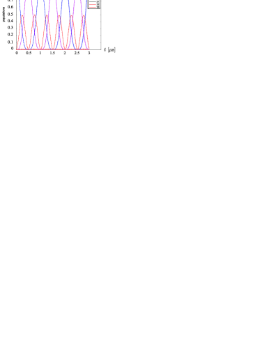
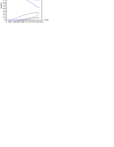
Figure 2: a) Evolution of the two-photon Fock state $\psi_{20}$ under the full Hamiltonian $H^{\prime}$ (solid lines) and the eliminated Hamiltonian $H_{\mathrm{eff}}$ (dashed lines) tuning the energies such that $\omega_{1}=\omega_{2}$ (beamsplitter-type interaction). b) Evolution of the state $\psi_{00}$ under the full Hamiltonian $H^{\prime}$ (solid lines) and the eliminated Hamiltonian $H_{\mathrm{eff}}$ (dashed blue lines) tuning the energies such that $\omega_{1}=-\omega_{2}$ (squeezing interaction). The dotted black lines show the evolution under exact two-mode squeezing (up to $n=3$).

Tuning the energies such that $\omega_{1}=-\omega_{2}$, the creation of a nuclear spin excitation is accompanied by scattering of a laser photon into the cavity, i.e. the effective coupling becomes $g_{2}(a^{\dagger}b^{\dagger}+ab)$ and the beamsplitter-type interaction $g_{1}(ab^{\dagger}+a^{\dagger}b)$ is off-resonant. The driving laser now facilitates the joint creation (or annihilation) of a spin excitation and a cavity photon, realizing a two-mode squeezing Hamiltonian

$$H_{\mathrm{sq}}=g_{2}(a^{\dagger}b^{\dagger}+ab)+\omega_{1}a^{\dagger}a+\omega_{2}b^{\dagger}b.$$ (4k)

The plots in figures 2a) and b) illustrate that the dynamics of the system can indeed be approximated by (4j) and (4k). To simulate the beamsplitter type coupling given by (4j), we choose $\omega_{1}=\omega_{2}$ and let the two-photon Fock state $\psi_{20}$ evolve under the Hamiltonian given by (4h) [see dashed lines in figure 2 a)]. Almost perfect Rabi-oscillations can be seen between the two-photon Fock state $\psi_{20}$ and the state with two nuclear spin excitations $\psi_{02}$, showing that $g_{2}(a^{\dagger}b^{\dagger}+\mathrm{h.c.})$ in (4h) can indeed be neglected. To simulate the squeezing-type interaction we choose $\omega_{1}=-\omega_{2}$ and study the evolution of the state $\psi_{00}$ under the Hamiltonian given by (4h) [see dashed blue lines in figure 2 b)]. It can be seen that the state $\psi_{00}$ evolves into the states $\psi_{11}$, $\psi_{22}$ and $\psi_{33}$ with coupling strengths $g_{2}\sqrt{n}$, depending on the number of excitations $n$. We have thus shown, that in this case, the beamsplitter-type interaction can indeed be neglected. For simplicity, we restricted the number of photons and nuclear excitations to $3$ in our simulation, such that states $\psi_{44}$ and higher excitation states do not occur and the evolution of the states $\psi_{22}$ and $\psi_{33}$ does only correspond to its evolution in a space with higher excitation numbers at very short times. This can be seen comparing the evolution to the exact two-mode squeezing which generates the state $\sqrt{1-\tanh^{2}{(g_{2}t)}}\sum_{n=0}^{\infty}\tanh^{n}{(g_{2}t)}\left|nn\right>$ for which the populations up to $n=3$ are plotted in figure 2 b) (dotted black lines).

4 Landau-Zener transitions

To map the state of the cavity to the nuclear spins, we take advantage of a formal analogy between the linear two-mode interaction given by (4j) in the Heisenberg picture and the Landau-Zener problem [22, 23]. In the conventional Landau-Zener problem, initially uncoupled Hamiltonian eigenstates of a two-level system interact at an avoided crossing. This interaction is achieved by slowly changing an external parameter such that the level separation is a linear function of time. If the system starts in the ground state, the probability of finding it in the excited state is given by the Landau-Zener formula [22, 23].

Here, we invoke this idea in the Heisenberg picture to achieve a mapping of the photon annihilation operator $a$ to the collective nuclear spin operator in the bosonic approximation $b$, i.e., $a\rightarrow b$ (the bosonic operators $a$ and $b$ are initially uncoupled). In the following we show that our system can be transformed to a system which corresponds to the standard Landau-Zener problem.

In the Heisenberg picture, the linear two-mode interaction between the cavity mode and the nuclear spins in the quantum dot, given by (4j), is described by a set of coupled differential equations for the mode operators:

$$\frac{\mathrm{d}}{\mathrm{dt}}\left(\begin{array}[]{c}a(t)\\ b(t)\end{array}\right)=-i\left(\begin{array}[]{cc}\omega_{1}&g_{1}\\ g_{1}&\omega_{2}\end{array}\right)\left(\begin{array}[]{c}a(t)\\ b(t)\end{array}\right).$$ (4l)

The available control parameters used to effect the change of $\omega_{1}-\omega_{2}$ are the laser Rabi frequency $\Omega_{l}$ and the laser frequency $\omega_{l}$. We consider a linear time dependence of

$$\omega_{1}-\omega_{2}=\beta t$$ (4m)

for simplicity while the coupling $g_{1}$ is constant.

Denoting by $a({u\choose v})$ the operator $ua_{-\infty}+vb_{-\infty}$ (a normalized linear combination of the purely photonic $a_{-\infty}$ and purely nuclear $b_{-\infty}$) and by $a_{t}({u\choose v})\equiv a({u_{t}\choose v_{t}})$ its image under time evolution, the two operator equations of (4l) can be combined into

$$\frac{d}{dt}a_{t}({u\choose v})=-ia_{t}\left[\left(\begin{array}[]{cc}\omega_{1}&g_{1}\\ g_{1}&\omega_{2}\end{array}\right){u\choose v}\right],$$

which can be written completely in terms of the mode function:

$$\frac{d}{dt}{u_{t}\choose v_{t}}=-i\left(\begin{array}[]{cc}\omega_{1}&g_{1}\\ g_{1}&\omega_{2}\end{array}\right){u_{t}\choose v_{t}}.$$ (4n)

This is the same kind of coupled differential equation that is encountered in the Landau-Zener problem [22, 23]. Following the calculation as done in [22, 23] we find that

$$|v(t=\infty)|^{2}=K^{2}U_{1}(\infty){U_{1}^{*}(\infty)}=1-\epsilon^{2},$$ (4o)

where $\epsilon\equiv e^{-\pi\gamma_{z}}$ and

$$\lim_{t\to\infty}U_{1}(t)=-K\frac{\sqrt{2\pi}}{\Gamma(i\gamma_{z}+1)}e^{-\frac{1}{4}\pi\gamma_{z}}e^{i\beta t^{2}}(\sqrt{\beta}t)^{i\gamma_{z}},$$ (4p)

with $\gamma_{z}=\frac{g_{1}^{2}}{\beta}$ and the constant $K=\sqrt{\gamma_{z}}\exp{\left(-\frac{\gamma_{z}\pi}{4}\right)}$ (for a detailed discussion see B). We thus find that the cavity mode operator $a$ is mapped to

$$a_{+\infty}=\sqrt{1-\epsilon^{2}}\,b_{-\infty}+\epsilon\,a_{-\infty},$$ (4q)

a dominantly nuclear operator for $\beta$ small enough so that $\epsilon$ is small, which effectively means for large enough times, as $\omega_{1}-\omega_{2}\equiv\beta t$.

4.1 Quality of the mapping for Fock and coherent states

In the following we will consider the quality of the mapping within the model given by (1) and (3), other imperfections will be discussed in Section 7. To evaluate the quality of the mapping, we return to the Schrödinger picture. The mapping of a $n$ photon Fock state of the cavity to the nuclei leads to a mixture of Fock states with photon numbers $\leq n$. The fidelity with which a $n$-photon Fock state is mapped, is given by

$$F_{\mathrm{F}}(n)=\left<n\right|\mathrm{tr}_{\mathrm{c}}\left(\left[\frac{a_{\infty}^{\dagger}}{\sqrt{n!}}\right]^{n}\left|0\right>\left<0\right|\left[\frac{a_{\infty}}{\sqrt{n!}}\right]^{n}\right)\left|n\right>=(1-\epsilon^{2})^{n},$$ (4r)

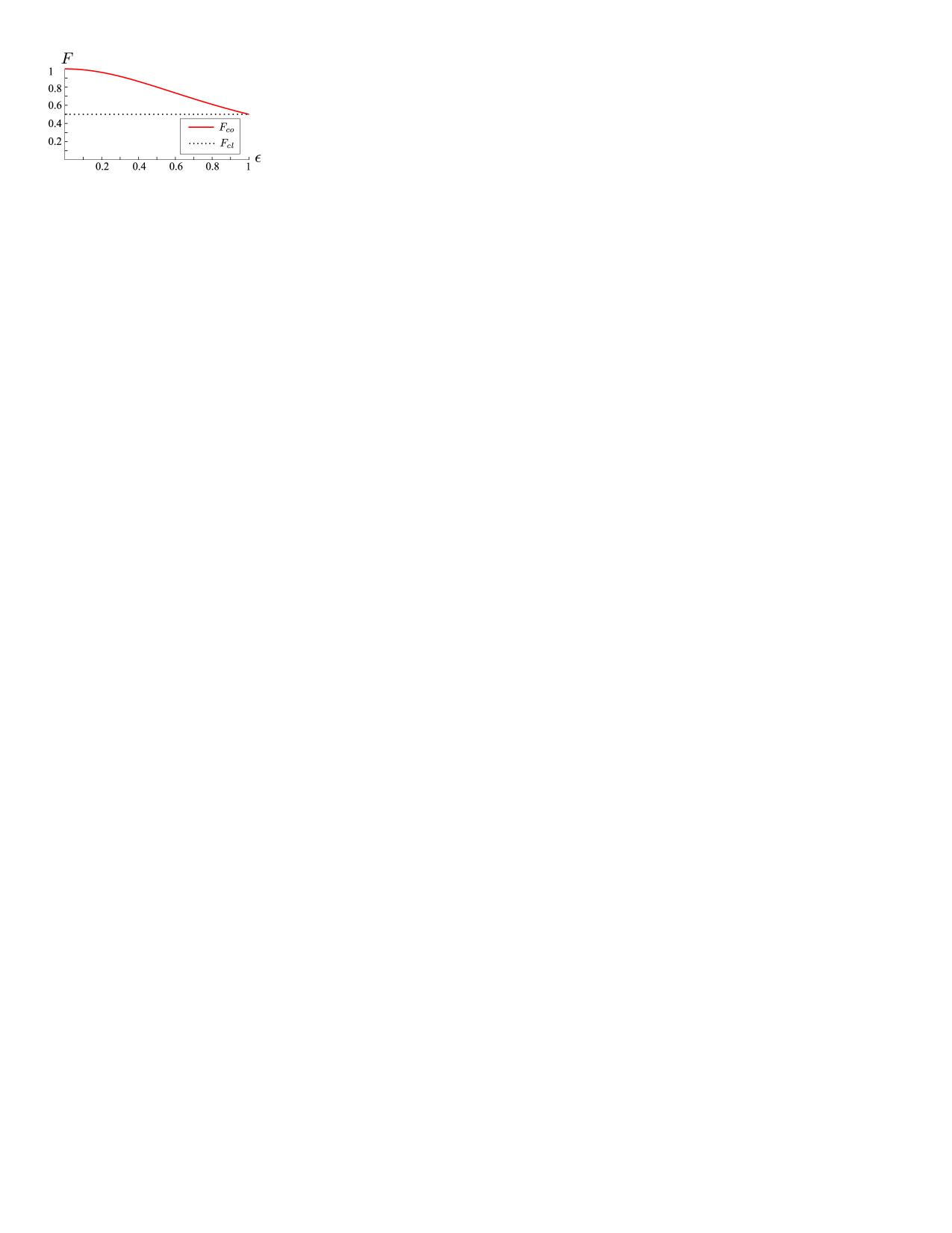
Figure 3: The (solid) red line indicates the fidelity of the mapping of an amplified coherent state of light to the nuclear spins vs the losses of the mapping $\epsilon$. The fidelity is, even for large losses, higher than the fidelity $F_{\mathrm{cl}}$ that can be achieved by classical means, indicated by the (dotted) black line.

where the cavity mode is traced out. In a next step, we want to know which fidelities can be achieved for superpositions of number states, e.g., for coherent states.

Coherent states are representatives of the family of Gaussian states, which play an important role in quantum optics and quantum information processing. A Gaussian state is fully characterized by its first and second moments $(\gamma,d)$, where $\gamma$ is the state’s covariance matrix and $d$ its displacement (see A). Since the dynamics generated by (4r) is Gaussian, the mapping can be fully characterized in terms of covariance matrices. The mapping of a Gaussian state of light onto the nuclear spins corresponds to

$$\left(\gamma_{c},d_{c}\right)_{\mathrm{c}}\stackrel{{\scriptstyle\mathrm{map}}}{{\longrightarrow}}\left((1-\epsilon^{2})\gamma_{c}+\epsilon^{2}\gamma_{ns}\,,\sqrt{1-\epsilon^{2}}d_{c}+\epsilon d_{ns}\right)_{\mathrm{ns}},$$ (4s)

where $(\gamma_{c},d_{c})_{\mathrm{c}}$ and $(\gamma_{ns},d_{ns})_{\mathrm{ns}}$ describe the states of cavity and nuclear spins, respectively. For a coherent state mapped to the nuclei, this corresponds to the map

$$\left(\mathbbm{1},\alpha\right)_{\mathrm{c}}\stackrel{{\scriptstyle\mathrm{map}}}{{\longrightarrow}}\left(\mathbbm{1},\sqrt{1-\epsilon^{2}}\alpha\right)_{\mathrm{ns}}.$$ (4t)

The fidelity of the mapping is given by [38]

$$F_{c}=|\langle\,\alpha\mid\sqrt{1-\epsilon^{2}}\alpha\,\rangle|^{2}=\exp\left[-\left|\left(1-\sqrt{1-\epsilon^{2}}\right)\alpha\right|^{2}\right].$$ (4u)

The minimal goal of a quantum interface is to achieve a better fidelity than can be achieved by classical means. As proved in [39, 40] the classical benchmark fidelity of coherent states distributed in phase space according to $p(\alpha)=\frac{\lambda}{\pi}\exp{(-\lambda|\alpha|^{2})}$ is given by $F_{max}=\frac{1+\lambda}{2+\lambda}$. Averaging $F_{c}$ over all possible coherent input states with a Gaussian distribution the fidelity reads

$$\overline{F_{c}}= \int\mathrm{d}^{2}\alpha\,p(\alpha)F_{c}=\frac{\lambda}{1-\epsilon^{2}/2-\sqrt{1-\epsilon^{2}}+\lambda}.$$ (4v)

For a flat distribution with $\lambda\rightarrow 0$ large photon numbers that lead to high losses are dominant and therefore $\overline{F_{c}}\rightarrow 0$.

A way to improve the average fidelity is to amplify the coherent state either at the write-in or the read-out stage, thus compensating losses due to the imperfect mapping. Optimal phase insensitive amplification would map $\left(\gamma,d\right)\longrightarrow\left(\kappa^{2}\gamma+(\kappa^{2}-1)\mathbbm{1},\kappa d\right)$ [41]. Choosing $\kappa$ such that $\kappa\stackrel{{\scriptstyle!}}{{=}}\frac{1}{\sqrt{1-\epsilon^{2}}}$, amplification and subsequent mapping can be written as

$$\left(\mathbbm{1},\alpha\right)_{\mathrm{c}}\stackrel{{\scriptstyle\mathrm{amp.}}}{{\longrightarrow}}\left(\kappa\,\mathbbm{1},\frac{1}{\sqrt{1-\epsilon^{2}}}\alpha\right)_{\mathrm{c}}\stackrel{{\scriptstyle\mathrm{map}}}{{\longrightarrow}}\left(\kappa(1-\epsilon^{2})+\epsilon^{2})\,\mathbbm{1},\alpha\right)_{\mathrm{ns}}.$$ (4w)

where subscript $c$ refers to the cavity and $ns$ to the nuclear spins. The fidelity of the mapping of the amplified state $\rho_{m}$, calculated using the relations for transition amplitudes of Gaussian states in [42], is given by

$$F_{\mathrm{co}} =\left<\alpha\right|\rho_{\mathrm{m}}(\alpha)\left|\alpha\right>=\det\left(\frac{\gamma_{c}+\gamma_{ns}}{2}\right)^{-1/2}e^{-(d_{ns}-d_{c})^{T}(\gamma_{c}+\gamma_{ns})(d_{ns}-d_{c})}$$ (4x)

$$=\det\left(\frac{\kappa(2-\epsilon^{2})+\epsilon^{2}}{2}\mathbbm{1}\right)^{-1/2}=\frac{1}{1+\epsilon^{2}}$$

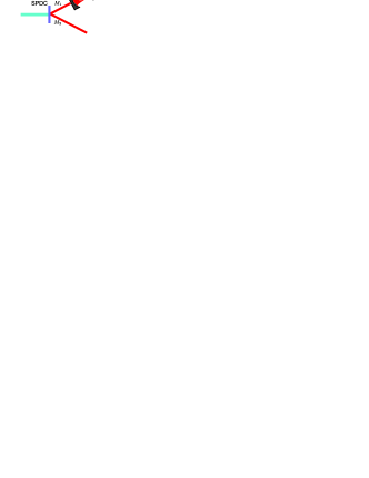
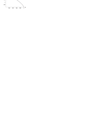
Figure 4: a) One part ($M_{1}$) of a two-mode squeezed state, arising from a Spontaneous Parametric Down Conversion source is coupled into the cavity and mapped to the nuclear spins of the quantum dot. Thereby, the other part ($M_{2}$) gets entangled with the nuclear spins. b) Plot of the Gaussian entanglement of formation (gEoF) for squeezing parameter $r=1$ vs mapping error $\epsilon$. The entanglement of the nuclear spins with part of a two-mode squeezed state ($M_{2}$) is a decreasing function for increasing mapping error $\epsilon$.

A plot of $F_{\mathrm{co}}$ is shown in figure 3. The fidelity of the mapping of the amplified coherent state is always higher than the classical benchmark fidelity $F_{\mathrm{cl}}=\frac{1}{2}$ for a flat distribution i.e., the quantum interface shows high performance even for large losses $\epsilon$.

4.2 Storage of an entangled state

Up to now we have shown that it is possible to transfer Fock and coherent states of light onto the nuclear spin memory. However, the ultimate test for a quantum memory is whether it is capable of faithfully storing part of an entangled quantum system. As an example for an entangled light state we consider a two-mode squeezed state where one of its light modes, $M_{1}$, is coupled into the cavity and mapped onto the nuclear spins of the quantum dot [see figure 4a)]. To see how well the entanglement is preserved, we compute the entanglement between the nuclear spins and the light mode $M_{2}$ using Gaussian entanglement of formation [43]. We find it to be a monotonically decreasing function of the mapping error $\epsilon\in[0,1]$. As seen from figure 4b) the nuclear spins of the quantum dot are entangled with the light mode $M_{2}$. This allows a remote access to the memory via teleportation, required for e.g., quantum repeaters.

4.3 Mapping time

A timescale for the mapping can directly be found considering Hamiltonian $H_{\mathrm{bs}}$ where the parameters are chosen such that $\omega_{1}=\omega_{2}$ and set to zero in a rotating frame: acting for a time $t=\pi/g$ (which is for the parameters used in Section 2 on the order of $6\mu$s) it maps $a\to b$ and $b\to a$ thus realizing a swap gate between cavity and nuclear spins. This setting however, would in contrast to the adiabatic methods discussed in this and the following Sections, be sensitive to timing errors because letting $H_{\mathrm{bs}}$ act for too long would reverse the mapping.

5 STIRAP

Mapping the state of the cavity to the nuclear spins is also possible considering a system where only the trion states are adiabatically eliminated and elimination of the electronic states is not required to achieve the desired interaction.

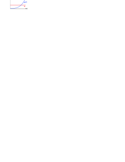
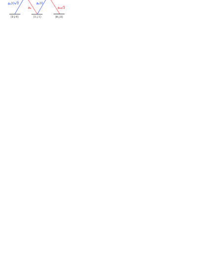
Figure 5: a) Schematic view of the time dependence of the coupling $g_{a}$ and the constant hyperfine coupling $g_{n}$. b) Schematic view of the level scheme of the system with initially two photons. The hyperfine coupling $g_{n}$ is ”always on”, whereas $g_{a}(t)$ is an increasing function for which $g_{a}(T)\gg g_{n}$.

We show that, with this system, the process of storing a state of light to the nuclear spins can be achieved by the well-known technique of Stimulated Raman Adiabatic Passage (STIRAP)[24], which has been studied for multilevel systems [44] and has been demonstrated in several experiments [24]. This scheme allows us to coherently transfer population between two suitable quantum states via a so-called counterintuitive sequence of coherent light pulses that drive transitions of a lambda or a multilevel system. It has some advantages over the Landau-Zener method as the choice of control parameters is easier and less constraints have to be fulfilled as we do not eliminate the electronic states, which allows for faster mapping times compared to the Landau-Zener method.

Note, that the main source of error, the decay of the cavity, is not considered here. Up to now, the experimentally achieved cavity decay rate $\gamma$ of a photonic crystal microcavity that couples to a quantum dot is of the order of $\gamma\approx 10^{10}\frac{1}{s}$ [45]. However, we do propose this scheme here, as cavity decay rates might improve and the scheme might also be used in a different setup.

For the system proposed in Section 2 the STIRAP method is not as straight forward as for the setup we investigated in [25] in Section V. The reason for this is, that after elimination of the trion states in the system used so far, there are two different couplings: $g_{a-}(S^{+}a^{\dagger}+h.c.)$ and $g_{a+}(S^{-}a^{\dagger}+h.c.)$, with $g_{a\pm}=\Omega_{c}\Omega_{l}/4\Delta_{T_{\pm}}$, where the first one has to be made off-resonant: $g_{a-}\gg g_{a+}$, which means that $\omega_{h}$ sets an upper limit to the coupling $g_{a+}$ (as the condition for the adiabatic elimination is $\Delta_{T_{\pm}}\gg\Omega_{c},\Omega_{l}$). Therefore, we study the STIRAP scheme for the system investigated in [25], where only the coupling $\propto(S^{-}a^{\dagger}+h.c.)$ is present.

In [25], we study a singly charged QD where the electronic states are Zeeman split by an external magnetic field in growth/$z$-direction (Faraday geometry). The electronic state $\left|\uparrow\right>$ is coupled to the trion state $\left|\Uparrow\right>$ (with angular momentum $+3/2$) by $\sigma^{+}$ circularly polarized light and the electronic state $\left|\downarrow\right>$ is coupled to the trion state $\left|\Downarrow\right>$ (with angular momentum $-3/2$) with $\sigma^{-}$-polarized light. These transitions can be stimulated by a $\sigma^{+}$-polarized cavity field and a $\sigma^{-}$-polarized classical laser field, respectively. The trion states are mixed with a resonant microwave field, whereas the electronic eigenstates are unchanged as they are far detuned from the microwave frequency and are now both coupled to the new trion eigenstates $\left|T_{\Uparrow}\right>=1/\sqrt{2}(\left|\Uparrow\right>-\left|\Downarrow\right>)$ and $\left|T_{\Downarrow}\right>=1/\sqrt{2}(\left|\Uparrow\right>+\left|\Downarrow\right>)$, and form a double $\Lambda$ system (see [25] for a figure).

In a frame rotating with the laser frequency the Hamiltonian reads

$$H = \frac{\Omega_{c}}{\sqrt{2}}\,(a^{\dagger}\,\left|\downarrow\right>\left<T_{\Uparrow}\right|-a^{\dagger}\,\left|\downarrow\right>\left<T_{\Downarrow}\right|+\mathrm{h.c.})+\frac{\Omega_{l}}{\sqrt{2}}(\left|\uparrow\right>\left<T_{\Uparrow}\right|+\left|\uparrow\right>\left<T_{\Downarrow}\right|+\mathrm{h.c.})$$ (4y)

$$+\delta^{\prime}a^{\dagger}a+\Delta_{+}\left|T_{\Uparrow}\right>\left<T_{\Uparrow}\right|+\Delta_{-}\left|T_{\Downarrow}\right>\left<T_{\Downarrow}\right|+\tilde{\omega}_{e}S^{z}+H_{\mathrm{hf}},$$

where $\delta^{\prime}=\omega_{c}-\omega_{l}-\omega_{mw}$ and $\Delta_{\pm}=\omega_{\Downarrow}-\omega_{l}\pm\Omega_{mw}$. Now, we derive the Hamiltonian where only the trion has been eliminated. If

$$\Delta_{\pm}\gg\Omega_{l},\Omega_{c}\sqrt{m}$$ (4z)

holds, the trion can be adiabatically eliminated. This leads to the Hamiltonian

$$H_{\mathrm{el}}= g_{a}\left(S^{+}a+\mathrm{h.c.}\right)+g_{n}\left(S^{+}b+\mathrm{h.c.}\right)+\frac{A}{2N}S^{z}b^{\dagger}b+\delta^{\prime}a^{\dagger}a+\tilde{\omega}_{e}S^{z}$$

$$+\left(\frac{\Omega_{c}^{2}}{2\Delta_{-}}+\frac{\Omega_{c}^{2}}{2\Delta_{+}}\right)a^{\dagger}a\left|\downarrow\right>\left<\downarrow\right|+\left(\frac{\Omega_{l}^{2}}{2\Delta_{-}}+\frac{\Omega_{l}^{2}}{2\Delta_{+}}\right)\left|\uparrow\right>\left<\uparrow\right|$$

where the coupling

$$g_{a}=\frac{\Omega_{c}\Omega_{l}}{2}\left(\frac{1}{\Delta_{+}}-\frac{1}{\Delta_{-}}\right).$$ (4ab)

We thus arrive, in addition to $H_{\mathrm{hf}}$, at an effective Jaynes-Cummings-like coupling of the two electronic spin states to the cavity mode governed by

$$g_{a}(S^{+}a+\mathrm{h.c.}),$$ (4ac)

i.e., the absorption of a cavity photon goes along with an upward flip of the electron spin (and the emission of a photon into the laser mode) and vice versa.

Next we present the STIRAP scheme: the couplings of the electronic states $\left|\uparrow\right>$ and $\left|\downarrow\right>$ are given by the optical fields ($g_{a}$) and the hyperfine coupling ($g_{n}$). The Hamiltonian describing the system is given by (5). It is blockdiagonal $H^{\prime}=\bigoplus_{m}H_{m}$, where $m$ denotes the initial photon number. The $(2m+1)$-dimensional Hamiltonian $H_{m}$, describing the evolution of the ”$m$-excitation subspace” can be written in the Fock basis $\{\left|m,\downarrow,0\right>,\left|m-1,\uparrow,0\right>,\left|m-1,\downarrow,1\right>,...\}$, where the first number $m-k$ represents the Fock state of the cavity, $\downarrow/\uparrow$ denotes the electron spin down/up state and $k$ the excitation number of the nuclear spins. In this basis, $H_{m}$ reads:

$$H_{m}=\left(\begin{array}[]{cccccc}\Delta_{G_{0}}&g_{a}\sqrt{m}&0&0&0&\ldots\\ g_{a}\sqrt{m}&\Delta_{E_{0}}&g_{n}\sqrt{1}&0&0&\ldots\\ 0&g_{n}\sqrt{1}&\Delta_{G1}&g_{a}\sqrt{m-1}&0&\ldots\\ 0&0&g_{a}\sqrt{m-1}&\Delta_{E_{1}}&g_{n}\sqrt{2}&\ldots\\ 0&0&0&g_{n}\sqrt{2}&\Delta_{G_{2}}&\ldots\\ \vdots&\vdots&\vdots&\vdots&\vdots&\ddots\end{array}\right),$$ (4aj)

with $\Delta_{G_{k}}=\left(\delta^{\prime}+\frac{\Omega_{c}^{2}}{2\Delta_{-}}+\frac{\Omega_{c}^{2}}{2\Delta_{+}}\right)(m-k)-\frac{A}{2N}k-\tilde{\omega}_{e}/2$, and $\Delta_{E_{l}}=\frac{\Omega_{l}^{2}}{2\Delta_{-}}+\frac{\Omega_{l}^{2}}{2\Delta_{+}}+\delta^{\prime}(m-l-1)+\frac{A}{2N}l+\tilde{\omega}_{e}/2$ for $k\in\{0,1,2..m\}$ and $l\in\{0,1,2..m-1\}$. In the following, we will denote the states with electron spin down as ”ground states”, $\left|G_{k}\right>=\left|m-k,\downarrow,k\right>$ and the ”excited states” by $\left|E_{l}\right>=\left|m-l-1,\uparrow,l\right>$. The optical fields couple states $G_{k}$ and $E_{l}$ with $k=l$ whereas states with $k=l+1$ are coupled by the hyperfine coupling (see figure 5b).

We will show in the following, that by slowly increasing the laser Rabi frequency and thus changing $g_{a}(t)$ such that $g_{a}(T)\gg g_{n}$, at the final time $T$ (see figure 5a), an initial state $\left|\psi,\downarrow,0\right>$ with no nuclear spin excitations in the quantum dot and a state $\left|\psi\right>$ in the cavity, evolves under the adiabatic change of $H^{\prime}$ to a state where the cavity is empty and its state has been mapped to the nuclear spins:

$$\left|\psi\downarrow 0\right>_{t=0}\rightarrow\left|0\downarrow\psi\right>_{t\rightarrow T}$$ (4ak)

for $T\rightarrow\infty$. A prerequisite for the mapping is, that the ground states of the Hamiltonian are all degenerate within each ”$m$-excitation”-subspace so that we can keep track of the phases of the individual eigenstates. This can be done by choosing the parameters such that $\Delta_{G_{k}}$ does not depend on $k$, which is fulfilled for $\delta+\frac{\Omega_{c}^{2}}{2\Delta_{-}}+\frac{\Omega_{c}^{2}}{2\Delta_{+}}=-\frac{A}{2N}-\tilde{\omega}_{e}/2$ so that $\Delta_{G_{k}}=-\frac{A}{2N}m-\tilde{\omega}_{e}/2$ . Hence, the phases $\phi_{m}=\Delta_{G_{m}}\,t$ of the individual eigenstates which the system acquires during the time evolution (for perfect adiabaticity) are known and can be corrected, e.g., by applying a magnetic field $-|B|\hat{z}$ for a time $t=\frac{A/(2N)}{g_{K}\mu_{K}|B|}$ after the state transfer to the nuclei. Here $g_{K}$ and $\mu_{K}$ denote the nuclear g-factor and the nuclear magnetic moment, respectively.

5.1 Numerical integration of the Schrödinger equation

To study the quality of the mapping of a state of the cavity to the nuclear spins, we numerically integrate the Schrödinger Equation given by

$$i\frac{\partial}{\partial t}\left|\psi(t)\right>=H^{\prime}(t)\left|\psi(t)\right>,$$ (4al)

where $H^{\prime}$ is the Hamiltonian given by (5). The simulation computes $\left|\psi(t+Dt)\right>=e^{-iH^{\prime}(t)Dt}\left|\psi(t)\right>$ in $T/Dt$ steps from $t=0$ to $t=T$. We assume, that the change of $g_{a}(t)$ is quadratic in time, ensuring an initially slow and a finally fast increase of $g_{a}(t)$ and $g_{a}(T)\gg g_{n}(T)$, $g_{a}=10\,g_{n}\frac{t^{2}}{T^{2}}$. Parameters are chosen as follows: we assume a hole g-factor $g_{h}=2.2$ and an electron g-factor $g_{e}=0.48$; the number of nuclei $N=10^{4}$, the hyperfine coupling constant $A=10\mu$eV, the laser and cavity Rabi frequency $\Omega_{c}=\Omega_{l}=13\mu$eV, the detuning of the trion $\omega_{\Downarrow}-\omega_{l}=103\mu$eV, the effective Zeeman splitting $\tilde{\omega}_{e}=0\mu$eV and the microwave Rabi frequency $\Omega_{mw}=50\mu eV$.

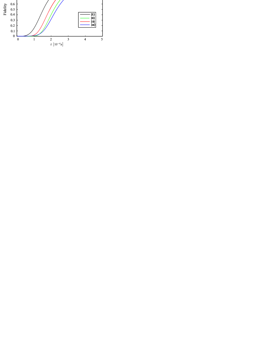
Figure 6: Plot of the fidelity of a variety of states vs time during the adiabatic evolution. $\left|1\right>$, $\left|2\right>$, $\left|3\right>$ denote the one, five, ten photon Fock states, respectively. $\left|\alpha\right>$ denotes the coherent state with average photon number $5$. The total evolution time is chosen to be $T=5\cdot 10^{-4}$s.

The fidelity of the mapping we are interested in is given by the overlap of the numerically evolved state $\rho(t)=\,\left|\psi_{\mathrm{si}}\right>\left<\psi_{\mathrm{si}}\right|$ and the ideal output $\left|\psi_{\mathrm{id}}\right>$

$$F=\left<\psi_{\mathrm{id}}\right|\rho(t)\left|\psi_{\mathrm{id}}\right>.$$ (4am)

To achieve a fidelity close to one, the total evolution time is chosen to be $T=5\cdot 10^{-4}$s. Figure 6 shows the fidelity plotted versus time for different kind of states that will be discussed in the following, illustrating the different aspects of mapping.

The one photon Fock state $\left|1\right>$ is mapped in $T=5\cdot 10^{-4}$s with a fidelity of $F\approx 0.99$ to the nuclear spins. To see that not only population but also relative phases are properly mapped we have simulated an approximately coherent state $\left|\alpha\right>=\exp{\left(-\frac{|\alpha|^{2}}{2}\right)}\sum_{k=0}^{20}\frac{\alpha^{k}}{\sqrt{k!}}\left|k\right>$ with average photon number $|\alpha|^{2}=5$ and find a mapping fidelity of $F\approx 0.96$. Here the known phases $\phi_{m}$ have been compensated.

5.2 Error processes

The main error processes that lead to imperfections of the fidelity are the ”always-on” character of the hyperfine coupling, the nonadiabaticity due to finite times, non-perfect polarization of the nuclei and the decay of the cavity. These processes will be studied in the following.

The fact that the hyperfine coupling is ”always-on” leads to an ”error” that is intrinsic to our system. Different to conventional STIRAP that uses overlapping light pulses, we propose to adiabatically increase the coupling $g_{a}(t)$ so that $g_{a}(T)\gg g_{n}$ and therefore the mapping is imperfect as $g_{n}$ is constant and can not be ”switched off”. Treating the coupling $g_{n}$ as a small perturbation in first order perturbation theory at $t=T$, the fidelity is found to be

$$F=\frac{|\langle\,\xi^{0}\mid\xi\,\rangle|^{2}}{\langle\,\xi\mid\xi\,\rangle}=\frac{1}{1+m\,g_{n}^{2}/{g_{a}(T)}^{2}}\approx 1-m\left(\frac{g_{n}}{g_{a}(T)}\right)^{2},$$ (4an)

where $\left|\xi^{0}\right>$ is the ideal output state for which $g_{n}=0$ (at t=T), and $\left|\xi\right>=\left|\xi^{0}\right>+\left|\xi^{1}\right>+..$ is the unnormalized eigenstate of $H_{m}$.

Another error arises from the non-adiabaticity due to finite times of realistic processes. For a quantitative estimate of the time $T$ that is needed for adiabatic passage to occur we use the well-known adiabatic theorem [46] and numerically compute the minimum time $T$ fulfilling

$$\frac{\mbox{$\mid\left<E_{l}^{m}(t)\right|\frac{\mathrm{d}}{\mathrm{dt}}(H^{\prime}-\bigoplus_{m}E_{G_{m}}\mathbbm{1})\left|\phi_{0}^{m}(t)\right>\mid$}}{\mbox{$\mid E_{l}\mid$}^{2}}\leq\delta_{\mathrm{a}}\,\,\forall\,t\,\in[\,0,\,T\,].$$ (4ao)

The left hand side of (4ao) corresponds to the probability to find the system in an excited state $\left|E_{l}^{m}\right>$ different from $\left|\phi_{0}^{m}\right>$ (the (purely nuclear) eigenstates to the eigenvalue $E=0$ of $H^{\prime}-\bigoplus_{m}E_{G_{m}}\mathbbm{1}$) and the fidelity decreases with $\delta_{\mathrm{a}}$. For $1/100<\delta_{\mathrm{a}}<1/10$ the minimum time fulfilling Equation (4ao) for the mapping of one photon is in the range of $1\mu s>T>0.11\mu s$.

To get an accurate description of the errors arising from non-adiabaticity we use a perturbative approach to treat nonadiabatic corrections and compute the phases arising from non-adiabaticity [47]. As the Hamiltonian $H^{\prime}=\bigoplus_{m}H_{m}$ is blockdiagonal, states with different initial photon numbers $m$ do not couple so that we can treat every ”$m$-photon” subspace separately. Moreover, we can use nondegenerate perturbation theory as the groundstates $\left|G_{k}\right>$ that are degenerate within each subspace are not coupled: $\left<G_{k^{\prime}}\right|\frac{\mathrm{d}}{\mathrm{dt}}H\left|G_{k}\right>$. Supposing to be at $t=0$ in one of the groundstates $\left|\phi_{G_{k}}(0)\right>$ of $H_{m}^{\prime}=H_{m}-E_{G_{m}}\mathbbm{1}$ slowly varying in time, the first order correction of the energy eigenvalue $E_{0}=0$ of $H$ is given by

$$E_{m}^{1}=\sum_{l\neq k}\frac{\mbox{$\mid\left<\phi_{E_{l}}\right|\frac{\mathrm{d}}{\mathrm{dt}}H_{m}^{\prime}\left|\phi_{G_{k}}\right>\mid$}^{2}}{E_{l}^{3}}.$$ (4ap)

The phases $\phi_{m}^{1}=\int_{0}^{T}\frac{E_{m}^{1}}{\hbar}\,\mathrm{dt}$ which the system acquires can be found by numerical integration of $E_{m}^{1}$. For $T=5\cdot 10^{-4}$s and initial photon number $m=1$, $\phi_{m}^{1}=-1.4\cdot 10^{-5}$ and for $m=2$, $\phi_{m}^{1}=0.004$, respectively. Thus, as expected, the errors arising from non-adiabaticity are small for sufficiently long times $T$.

6 Quantum Interface in the bad cavity limit

In the previous Sections, we have shown that a quantum interface can be achieved via direct mapping of the cavity field to the nuclear spins of the QD.

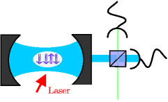
Figure 7: Quantum teleportation can be used to write the state of a traveling-wave light field onto the nuclei.

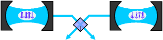
Figure 8: Nuclear spins of quantum dots in two distant cavities can be entangled by interfering the travelling wave output fields of the two cavities at a beamsplitter and measuring.

But we have also seen that the cavity lifetimes required for high-fidelity storage are much larger than what is today’s state of the art, i.e., as $g_{1,2}\ll 1/\tau_{\mathrm{cavity}}$, we are, compared to the effective coupling, in the “bad cavity limit”. A second problem with this approach is that the quantum information we want to map to the nuclei has to be coupled into a high-Q cavity. This is notoriously difficult although theoretical proposals exist [3] that should avoid reflection completely. Both problems can be circumvented employing ideas similar to [48, 49] by using the two-mode squeezing Hamiltonian $H_{\mathrm{sq}}$ [see (4k)] (note that we now return to the system proposed in Section 2 for the rest of the paper). As discussed in [25] and elaborated in more detail below, it is possible to create entanglement between nuclei and the traveling-wave output field of the cavity. Then, quantum teleportation can be used to write the state of another traveling-wave light field onto the nuclei (figure 7) . This approach gives an active role to cavity decay in the interface and can tolerate a bad effective cavity as long as strong coupling is achieved in (4e). Moreover, it does not require to couple the quantum information into the cavity. Similarly $H_{\mathrm{bs}}$ [(4j)] enables read-out, by writing the state of the nuclei to the output field of the cavity. The entanglement between nuclear spins and output field can moreover be used to entangle nuclear spins in two distant cavities by interfering the output light of the cavities at a beamsplitter (figure 8).

6.1 Entangling nuclei with the output field

The Hamiltonian of the nuclear spin-cavity system tuned to the squeezing interaction (4k) and coupled to the environment is given by

$$H=g_{2}(a^{\dagger}b^{\dagger}+ab)+ia\int\sqrt{\frac{\gamma}{2\pi}}c_{\omega}^{\dagger}\,d\omega+\mathrm{h.c.}+\int\omega c^{\dagger}_{\omega}c_{\omega}d\omega,$$ (4aq)

where $c_{\omega}$ are the annihilation operators of the bath and $\gamma$ the cavity decay constant. We have specialized (4k) to the case $\omega_{1}=-\omega_{2}$ and transformed to an interaction picture with $H_{0}=\omega_{1}(a^{\dagger}a-b^{\dagger}b)+\omega_{1}\int c^{\dagger}_{\omega}c_{\omega}d\omega$ and performed the rotating-wave and Markov approximations in the description of the cavity decay [51]. The quantum Langevin equations of cavity and nuclear operators read

$$\dot{a}(t) = -ig_{2}\,b^{\dagger}(t)-\frac{\gamma}{2}a(t)-\sqrt{\gamma}c_{\mathrm{in}}(t)$$ (4ara)

$$\dot{b}(t) = -ig_{2}\,a^{\dagger}(t).$$ (4arb)

Here, $c_{\mathrm{in}}$ describes the vacuum noise coupled into the cavity and satisfies $[c_{\mathrm{in}}(t),c_{\mathrm{in}}^{\dagger}(t^{\prime})]=\delta(t-t^{\prime})$. The solutions of (4ara) and (4arb) are given (for $t\geq 0$) by

$$a(t) = p_{-}(t)a(0)+q(t)b^{\dagger}(0)+\sqrt{\gamma}\int_{0}^{t}p_{-}(t-\tau)c_{\mathrm{in}}(\tau)d\tau$$ (4arasa)

$$b(t) = q(t)a^{\dagger}(0)+p_{+}(t)b(0)+\sqrt{\gamma}\int_{0}^{t}q(t-\tau)c_{\mathrm{in}}^{\dagger}(\tau)d\tau$$ (4arasb)

where

$$p_{\pm}= e^{-\frac{1}{4}t\gamma}\left[\cosh{\left(\nu t\right)}\pm\frac{\gamma}{4\nu}\sinh{\left(\nu t\right)}\right],$$ (4arasat)

$$q= -i\frac{g_{2}}{\nu}e^{-\frac{1}{4}\gamma t}\sinh{\nu t},$$ (4arasau)

with

$$\nu=\sqrt{\left(\frac{\gamma}{4}\right)^{2}+g_{2}^{2}}.$$ (4arasav)

While (4arasa) and (4arasb) describe a non-unitary time-evolution of the open cavity-nuclei system, the overall dynamics of system plus surrounding free field given by the Hamiltonian in (4aq) is unitary. Moreover, it is Gaussian (see A), since all involved Hamiltonians are quadratic. Since all initial states are Gaussian (vacuum), the joint state of cavity, nuclei, and output fields is a pure Gaussian state at all times as well. This simplifies the analysis of the dynamics and in particular the entanglement properties significantly: The covariance matrix [defined by (4arasaybzcd) in A] of the system allows us to determine the entanglement of one part of the system with another one. In particular, we are interested in the entanglement properties of the nuclei with the output field.

The covariance matrix $\Gamma_{\mathrm{ns-c-o}}$ of the pure Gaussian state of nuclear spins, cavity and output field and thus the covariance matrix $\Gamma_{\mathrm{ns-o}}$ of the reduced nuclei-output field system can be found by analyzing the covariance matrix of the cavity-nuclei system $\Gamma_{\mathrm{ns-c}}$.

The elements $\left<X\right>$ of the covariance matrix $\Gamma_{\mathrm{ns-c}}$ can be calculated by solving the Lindblad equation evaluated for the expectation values $\left<X\right>$

$$\frac{d}{dt}\left<X\right>=i\left<[H_{\mathrm{sq}},X]\right>+\frac{\gamma}{2}\left(\left<2a^{\dagger}Xa\right>-\left<Xa^{\dagger}a\right>-\left<a^{\dagger}aX\right>\right).$$ (4arasaw)

We thus find the covariance matrix of the cavity-nuclei system to be

$$\Gamma_{\mathrm{ns-c}}=\left(\begin{array}[]{cccccccc}m&0&0&k\\ 0&m&k&0\\ 0&k&n&0\\ k&0&0&n\end{array}\right),$$ (4arasax)

where

$$m = e^{-\frac{\gamma t}{2}}\left[\frac{\gamma}{\nu}\sinh{\left(2\nu t\right)}\right.\left.+\left(\frac{g_{2}^{2}}{\nu^{2}}+\frac{\gamma^{2}}{8\nu^{2}}\right)\cosh{\left(2\nu t\right)}+\frac{g_{2}^{2}}{\nu^{2}}\right]-1,$$ (4arasaya)

$$n = 1+32\frac{g_{2}^{2}}{\nu^{2}}e^{-\frac{\gamma t}{2}}\sinh{\left(\nu t\right)}^{2},$$ (4arasayb)

$$k = e^{-\frac{\gamma t}{2}}\left[\frac{g_{2}\gamma}{2\nu^{2}}\sinh{\left(\nu t\right)}^{2}+\frac{g_{2}}{\nu}\sinh{\left(2\nu t\right)}\right].$$ (4arasayc)

According to [52] there exists a symplectic transformation $S$ (cf. A) such that $\Gamma_{\mathrm{D}}=S\Gamma_{\mathrm{ns-c}}S^{T}=\mathrm{diag}(\lambda^{s}_{1},\lambda^{s}_{1},\lambda^{s}_{2},\lambda^{s}_{2})$ where $\{\lambda^{s}_{1},\lambda^{s}_{2}\}$ are the symplectic eigenvalues of $\Gamma_{\mathrm{ns-c}}$. This allows us to calculate the covariance matrix of the pure nuclei-cavity-output field system

$$\Gamma_{\mathrm{ns-c-o}}=S^{\prime}\Gamma_{\mathrm{D^{\prime}}}(S^{\prime-1})^{T}$$ (4arasayaz)

with $\Gamma_{\mathrm{D^{\prime}}}$ in $2\times 2$ block-matrix form

$$\Gamma_{\mathrm{D^{\prime}}}=\left(\begin{array}[]{cccc}\cosh{(2r_{1})}\mathbbm{1}_{2}&&\sinh{(2r_{1})}\sigma_{z}&\\ &\cosh{(2r_{2})}\mathbbm{1}_{2}&&\sinh{(2r_{2})}\sigma_{z}\\ \sinh{(2r_{1})}\sigma_{z}&&\cosh{(2r_{1})}\mathbbm{1}_{2}&\\ &\sinh{(2r_{2})}\sigma_{z}&&\cosh{(2r_{2})}\mathbbm{1}_{2}\end{array}\right),$$ (4arasayba)

where $\cosh{r_{1}}=\lambda^{s}_{1}$ and $\cosh{r_{2}}=\lambda^{s}_{2}$ and $S^{\prime}=\left(\begin{array}[]{cc}S&\\ &\mathbbm{1}_{4\times 4}\end{array}\right)$. One of the symplectic eigenvalues $\{\lambda^{s}_{1},\lambda^{s}_{2}\}$ is 1, indicating a pure - and therefore unentangled - mode in the system. That implies that there is a single “output mode” in the out-field of the cavity to which the cavity-nuclear–system is entangled and we can thus trace out the unentangled output mode.

The procedure for entangling the nuclei with the output field (write-in) is: let $H_{\mathrm{sq}}$ act for time $t_{1}$ to create a two-mode squeezed state $\psi(g_{2},t_{1})$: nuclei entangled with cavity and output field. To obtain a state in which the nuclei are only entangled to the output field, we switch the driving laser off $(g_{2}=0)$ and let the cavity decay for a time $t_{2}\gg\tau_{\mathrm{cav}}$, obtaining an almost pure two-mode squeezed state of nuclei and the output mode. We define the coupling as

$$g_{t}=\cases{g_{2},t<t_{1}}{0,t\geq t_{1}}$$ (4arasaybb)

For the parameters used in Section 3, $g_{2}\sim 1.9\cdot 10^{-3}\mu$eV.

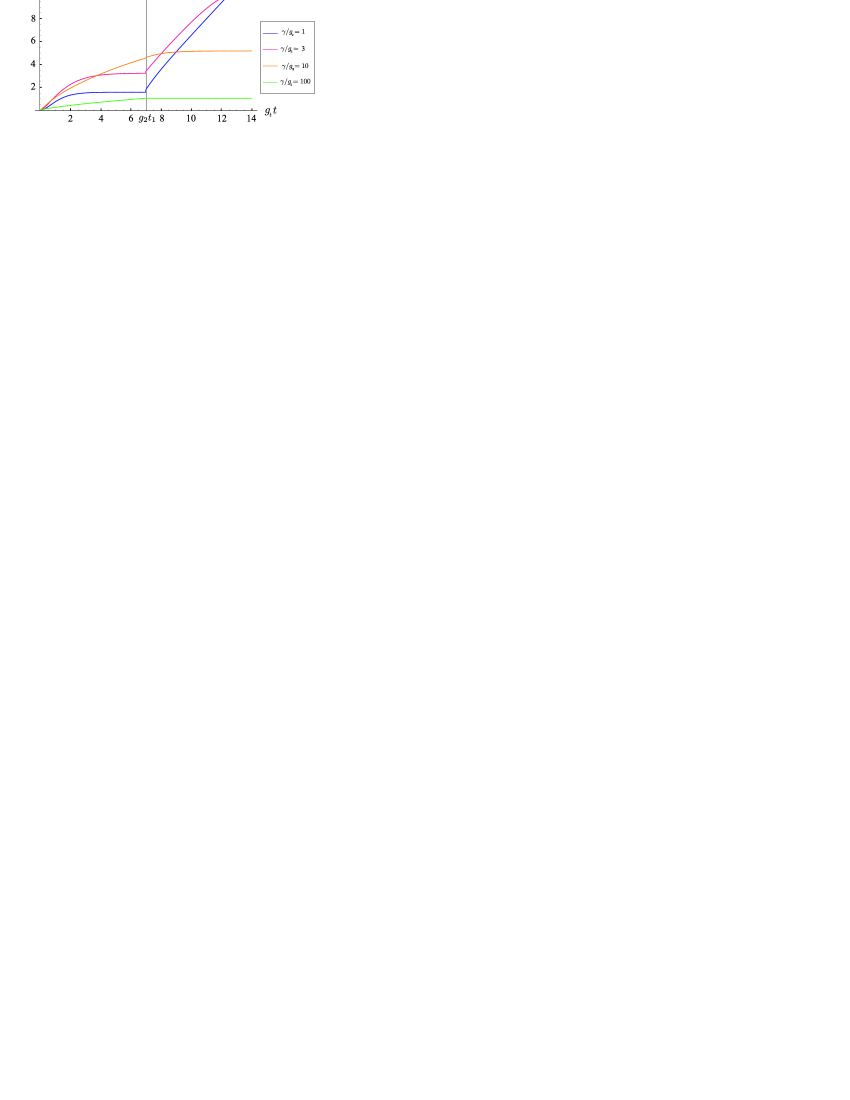
Figure 9: Plot of the Gaussian entanglement of formation (gEoF) of the nuclei with the output field vs $t$ for different values of $\gamma/g$. At $g_{2}t_{1}=7$ the coupling is switched off. The curve saturates when all excitations have leaked out of the cavity.

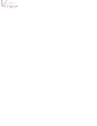
Figure 10: a) Plot of the entanglement entropy $S_{E}$ of the nuclei+cavity with the output field vs $t$ for different values of $\gamma/g$. At $g_{2}t_{1}=7$ the coupling is switched off. b) Plot of the entanglement entropy $S_{E}$ of the nuclei with the cavity+output field vs $g_{2}t$ for different values of $\gamma/g_{2}$.

The entanglement of the different subsystems can be quantified: We compute the Gaussian entanglement of formation (gEoF) [43] of the reduced covariance matrix of the nuclei-output field–system to quantify the entanglement of the nuclei with the output field (see figure 9). The gEoF measures how costly it is to generate a state by mixing pure Gaussian states. It gives an upper bound to the entanglement of formation (EoF) and is in the present case equivalent to the logarithmic negativity [53]. The entanglement of the pure cavity-nuclei-output mode–system can be quantified using the entanglement entropy $S_{E}$ [54]. We plot $S_{E}$ for the nuclei-cavity system with the output mode [see figure 10a)] and of the nuclei with the cavity-output mode–system [see figure 10b)]. The entanglement is plotted versus $g_{2}t$ for different ratios of the cavity decay constants and the coupling, $\gamma/g_{2}$.

6.2 Write-in: Teleportation channel

The entangled state between nuclei and the cavity output field allows us to map a state of a traveling light field to the nuclei using teleportation (see figure 7) [26].

To realize the teleportation, a Bell measurement has to be performed on the output mode of the cavity and the signal state to be teleported. This is achieved by sending the two states through a 50:50 beam splitter and measuring the output quadratures [26]. To be able to do this, we need to know $B_{0}$, the output mode of the cavity. In the following, we derive an exact expression for this mode.

We fix a time $t$ and denote by $B(y,t)$, $y\in\mathbb{N}$ a complete set of bath modes outside the cavity. $B(y,t)$ can be expressed as a superposition of bath operators $c(x,t)$

$$B(y,t)=\int z(y,x,t)c(x,t)dx$$ (4arasaybc)

where we introduce a complete set of orthonormal mode functions $z(y,x,t)$. The bath operators $c(x,t)$ are known from the input-output relations [51]

$$c(x,t)=\frac{\sqrt{\gamma}}{2}a(t-x)\chi_{[0,t]}(x),$$ (4arasaybd)

where $a(t)$ is given by (4arasa). To calculate $B(y,t)$ we thus need to determine $z(y,x,t)$. This can be done, calculating the variance $\left<c^{\dagger}(x,t),c(x^{\prime},t)\right>=\left<c^{\dagger}(x,t)c(x^{\prime},t)\right>-\left<c^{\dagger}(x,t)\right>\left<c(x^{\prime},t)\right>$ following two different pathways: With (4arasaybd) we find

$$\left<c^{\dagger}(x,t),c(x^{\prime},t)\right>=\frac{\gamma}{4}q(t-x^{\prime})q(t-x)^{*},$$ (4arasaybe)

where $q(t)$ is given by (4arasau). Another way to express $c(x,t)$ follows from (4arasaybc):

$$c(x,t)=\sum_{y}z(y,x,t)^{*}B(y,t).$$ (4arasaybf)

As shown in Section 6.1 there exists only one output mode which we label $y=0$. This mode contains all the output photons. Therefore $\left<B(y,t)^{\dagger}B(y^{\prime},t)\right>=K\,\delta_{y0}\delta_{y^{\prime}0}$ and the variance using (4arasaybf) reads

$$\left<c^{\dagger}(x,t),c(x^{\prime},t)\right>=K\,z(0,x,t)z(0,x^{\prime},t)^{*}.$$ (4arasaybg)

Comparing (4arasaybe) to (4arasaybg) we find

$$z(0,x,t)=\frac{q(t-x)^{*}}{\sqrt{\int|q(t-x)|^{2}dx}}$$ (4arasaybh)

and $K=\frac{\gamma}{4}\sqrt{\int|q(t-x)|^{2}dx}$ and we have thus fully determined $B(0,t)$ (see figure 13). Note that the bath modes are given in a frame rotating with $\omega_{1}+\omega_{l}$ to which we transformed in Section 2 ($\omega_{l}$) and Section 6 ($\omega_{1}$).

Therefore a state of a traveling light field can be teleported to the nuclear spins up to a random displacement that arises from the teleportation protocol [55, 26]. The random displacement can be undone, letting the beam-splitter interaction $H_{bs}$ [given by (4j)] act for a short time, while pumping the cavity with intense coherent light as suggested in [50].

Next, we want to consider the quality of the teleportation. Whereas before (see figures 9 and 10) the time evolution of the system for a fixed switch-off time $g_{2}t_{1}=7$ was considered, we now consider the ”final” entangled state of nuclei and output field depending on $g_{2}t_{1}$, where the cavity has decayed to the vacuum state while the nuclei are (still) stationary.

The fidelity with which a quantum state can be teleported onto the nuclei is a monotonic function of the two-mode squeezing parameter

$$r_{1}=\frac{1}{2}\mathrm{arccosh(\textit{$m(t=t_{1})$})}$$ (4arasaybi)

with $m$ defined in (4arasaya). A typical benchmark [39] is the average fidelity with which an arbitrary coherent state can be mapped. This fidelity has a simple dependence on the two-mode squeezing parameter $r_{1}$ of the state used for teleportation and is given by [56]

$$F_{\mathrm{tel}}=\frac{1}{1+e^{-2r_{1}}}.$$ (4arasaybj)

We plot the teleportation fidelity dependent on the switch-off time

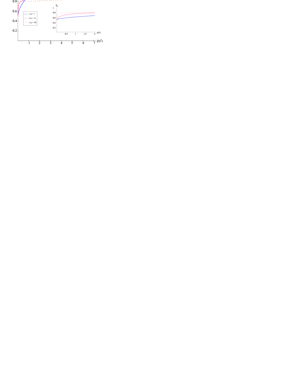
Figure 11: Plot of the teleportation fidelity vs $g_{2}t_{1}$ for different values of $\gamma/g_{2}$.

$t_{1}$ (see figure 11).

Already for $r_{1}(t_{1})\sim 1$ fidelities above $0.8$ are obtained. After switching off the coupling we have to wait for the cavity to decay which typically happens on a nanosecond timescale and does not noticeably prolong the protocol.

6.3 Read-out

The beamsplitter Hamiltonian $H_{\mathrm{bs}}$ [given by (4j)] enables read-out of the state of the nuclei by writing it to the output field of the cavity. The quantum Langevin equations of cavity and nuclear operators lead to almost identical solutions as for $H_{\mathrm{sq}}$ [see (4arasa) and (4arasb)]: of course, now $a(t)$ is coupled to $b(t)$ instead of $b^{\dagger}(t)$ but the only other change to (4arasa) and (4arasb) is to replace $\nu$ by

$$\tilde{\nu}=\sqrt{(\gamma/4)^{2}-g_{1}^{2}}.$$ (4arasaybk)

This has the effect that all terms in (4arasa)and (4arasb) show exponential decay with $t$. The decay of the slowest terms $\sim e^{-2\frac{g_{1}^{2}}{\gamma}t}$ sets the timescale for read-out. To calculate the read-out fidelity, we need to know the state of the output field at time $t=T$. We assume that the state we want to read-out is a coherent state with displacement $\alpha_{\mathrm{ns}}$ at time $t=0$ fully described by its covariance matrix $\gamma_{b}(0)=\mathbbm{1}$ and its displacement $d_{b}(0)=\left<b\right>=\alpha_{\mathrm{ns}}$ (while cavity and output field are in the vacuum state at $t=0$). As the norm of the displacement $\|d(t)\|$ of the nuclei-cavity-output system

$$d(t)=\left(\begin{array}[]{c}d_{a}(t)\\ d_{b}(t)\\ d_{B_{0}}(t)\end{array}\right)=\left(\begin{array}[]{c}\left<a(t)\right>\\ \left<b(t)\right>\\ \left<B_{0}(t)\right>\end{array}\right)$$ (4arasaybl)

does not change under the beamsplitter transformation, the displacement of the output mode $B_{0}$ is given by

$$|d_{B_{0}}(t)| =\sqrt{\|d(0)\|^{2}-d_{a}(t)^{2}-d_{b}(t)^{2}}$$ (4arasaybm)

$$=\sqrt{1-(|q(t)|^{2}+|p_{+}(t)|^{2})}|\alpha_{\mathrm{ns}}|$$

where $q(t)$ and $p_{+}(t)$ are defined by (4arasa) and (4arasb) with $\nu$ replaced by $\tilde{\nu}$.

At finite times, the nuclear excitations and the cavity have not fully decayed which leads to a loss of amplitude of the mapped state. The loss is very small for sufficiently large $T$. To assure high fidelity even for states with large photon number, we can amplify the output field as in Section 4.1. Then the state of the output field is $(\gamma_{B_{0}},d_{B_{0}})=(\kappa\mathbbm{1},\alpha_{\mathrm{ns}})$ with $\kappa$ as defined in Section 4.1. This leads to a read-out fidelity (see figure 12) given by

$$F_{\mathrm{read}}= \mbox{$\mid\langle\,\mathbbm{1},\alpha_{\mathrm{ns}}\mid\,\kappa\mathbbm{1},\alpha_{\mathrm{ns}}\,\rangle\mid$}^{2}=1-(|q|^{2}+|p_{+}|^{2}),$$

where we have used relations for the transition amplitudes (as in Section 4.1) given by [42].

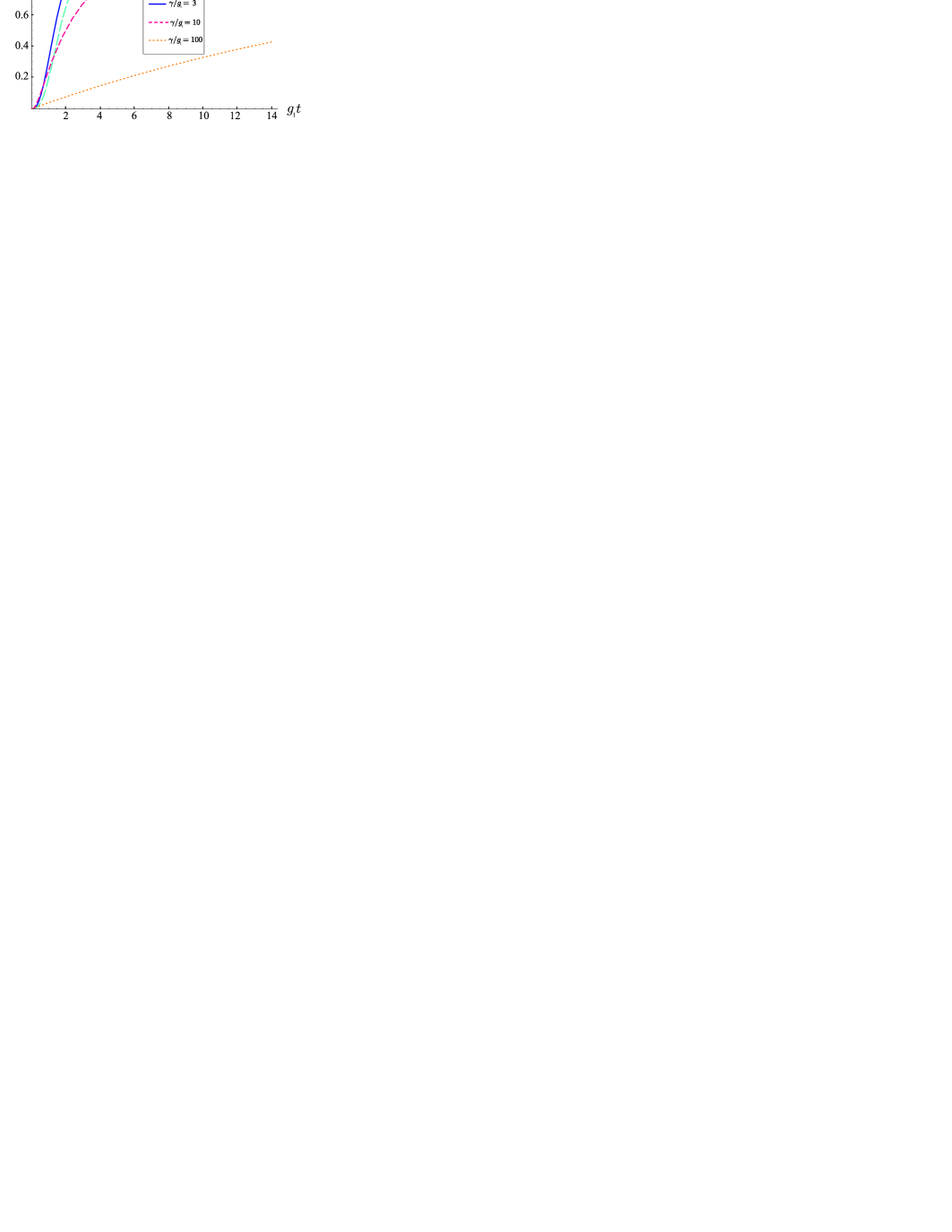
Figure 12: Plot of the read-out fidelity vs $g_{1}t$ for different values of $\gamma/g_{1}$

6.4 Output mode

In figure 13 we plot the output mode of the cavity given by (4arasaybc) for write-in and read-out, respectively, and for several choices of the parameters $g_{1,2}$ and $\gamma$. We are considering here only the idealized case of a one-sided and one-dimensional cavity. In general, the actual geometry of the cavity at hand has to be taken into account to determine $B_{0}$. In the following we briefly discuss the shape of the mode-function. It provides some insight into the dynamics of the mapping process, since due to (4arasaybd) the weight of $c(x,T)$ in $B(0,t)$ reflects the state of the cavity mode at time $t-x$ in the past.

Write-in: Let us consider the two extreme cases of very strong and very weak cavity decay. In the former case ($\gamma\gg g_{2}$) the cavity mode can be eliminated, i.e., the nuclear spins couple directly and with constant strength $\sim g_{2}^{2}/\gamma$ to the output field: $z_{0}$ is a stepfunction which is $0$ for $g_{2}=0$ and constant otherwise. This is reflected in figure 13, where for $\gamma=100g_{2}$ most of the excitations decay directly to the outputmode such that $z_{0}$ takes a ”large” value at the time the squeezing is switched on and then increases only slowly in time. After switching the squeezing interaction off the cavity quickly decays to the vacuum. For $\gamma\ll g_{2}$, instead, two-mode squeezing builds up in the nuclei–cavity system as long as the squeezing interaction is on ($3\mu$s in figure 13) and after $g_{2}$ is switched off the cavity decays to its standard exponential output mode. The intermediate cases in figure 13a) show the shifting weight between “initial step-function” and subsequent exponential decay.

Read-out: In the case of the beamsplitter interaction, the same cases can be distinguished. For large $\gamma/g_{1}$, the cavity can be eliminated and the nuclear spins are mapped directly to the exponential output mode of a cavity decaying with an effective rate $g_{1}^{2}/\gamma$. For smaller $\gamma$, the output mode reflects the damped free evolution of the nuclei–cavity system, which in this case includes oscillations (excitations are mapped back and forth between nuclei and cavity at rate $g_{1}$) in absolute value and phase.

Figure 13: The output mode in one dimension: Plot of $z_{0}$ vs position $x$, where $x=0$ is the position of the cavity a) Write-in: The squeezing interaction is ”on” for $3\mu$s and then switched off. b) Read-out: For $\gamma\gg g_{2}$ the excitations do not have fully decayed to the output mode after $t=12\mu$s. The read-out fidelity given by (6.3) corresponds to the probability that the excitations in the nuclear spins have decayed into the output mode of the cavity. For $\gamma/g_{1}=1$ and $\gamma/g_{1}=10$ the read-out fidelity is $F_{\mathrm{read}}>0.98$ after $t\approx 16-20\mu$s. For $\gamma/g_{1}=100$ however, it takes $\approx 200\mu$s to achieve $F_{\mathrm{read}}>0.98$. Note that for input and output modes that have similar shapes (e.g. for a network), it is best to consider the case where $\gamma/g_{1}\gg 1$.)

6.5 Linear Optics with the Nuclear Spin Mode

The interaction we have described can not only be used to map states to the nuclear spin ensemble but also for state generation and transformation. In fact, from a nuclear spin mode in the vacuum state, all single mode Gaussian states can be prepared. To see this, we have to show how any desired $2\times 2$ correlation matrix $\Gamma$ and displacement $d\in\mathbbm{C}$ can be obtained.

As we remarked already when discussing the write-in via teleportation, the beam-splitter Hamiltonian $H_{\mathrm{bs}}$ can be used to realize displacements of the nuclear mode. Driving the cavity mode with a strong laser to a coherent state with amplitude $\alpha$ (and the same phase as $d$) and switching on $H_{\mathrm{bs}}$ for a time $t=|\beta|/(g_{1}|\alpha|)$ provides in the limit of large $\alpha$ a good approximation to the displacement operation by $\beta$ [50].

Concerning the CM, we use that every CM of a pure Gaussian state is of the form $\Gamma=ODO^{T}$, where $D$ is a positive diagonal matrix with determinant one and $O$ is orthogonal and symplectic. $O$ can be seen as the effect of time evolution under some quadratic Hamiltonian acting on the single-mode squeezed state with CM $D$. In the single mode case, any $O$ represents a phase shift and is obtained by letting the nuclear system evolve “freely” (without laser coupling, i.e. a polarized electron interacts off-resonantly with the nuclei) according to the Hamiltonian $\propto b^{\dagger}b$ for some time. Thus the state with CM $\Gamma$ can be generated in a two-step process: first generate the state with $\Gamma=D$, then apply $O$.

While in the preceding paragraphs we could show how to realize operations that can act on any input state, no such possibility seems to exist for squeezing in our context. Instead we show how to obtain the pure single mode squeezed state with CM $D$ from the vacuum state. Letting $H_{\mathrm{sq}}$ act on the vacuum results in a two-mode squeezed state with squeezing parameter $r_{2}$. Performing a homodyne measurement (of the $X$ quadrature) on the optical part of this state projects the nuclear system into a squeezed state with squeezing $r_{1}=\ln[\cosh(2r_{2})]/2$ [57], thus given enough two-mode squeezing, any CM $D$ can be produced.

One can go even further and simulate evolution according to any quadratic Hamiltonian on the nuclear-optical system: According to [58], the Hamiltonian given by (4h) with the interaction part $g_{1}ab^{\dagger}+g_{2}a^{\dagger}b^{\dagger}+\mathrm{h.c.}$ enables simulation of any Hamiltonian quadratic in $a,b,a^{\dagger},b^{\dagger}$.

7 Remarks on internal nuclear dynamics and approximations

With regard to the realization of the proposed protocol and the applicability of the approximations leading to the Hamiltonians (4j), (4k) there are three aspects to consider: spontaneous emission of the quantum dot, the internal nuclear dynamics and errors in the bosonic description. We assume the strong coupling limit of cavity-QED and neglect spontaneous emission of the quantum dot. The other two aspects will be studied in the following. Note that the results on the internal nuclear dynamics are corroborated by independent work of Kurucz et al. [59]. They introduce the bosonic description to analyze the performance of a nuclear spin quantum memory and show that the performance of the memory is enhanced due to a detuning between excitations in the mode $b$ versus those in other modes $b_{k\not=0}$ and that secular dipolar terms do not affect the memory.

7.1 Internal nuclear dynamics

Up to now, we have focused exclusively on the hyperfine interaction and neglected “internal” nuclear dynamics, dominated by dipolar and quadrupolar interactions. Moreover, the hyperfine coupling leads to a dipolar interaction between nuclei mediated by the electron. We study the dipolar interaction between nuclear spins which is significantly weaker than $g_{n}$, $g_{1}$ and $g_{2}$: the energy scale for dipolar interaction between two nuclei has been estimated $\sim 10^{-5}\mu$eV for GaAs [27]. However, since for $10^{4}-10^{6}$ nuclei there are many of these terms, they might play a role at the $10-50\mu$s time scales considered.

7.1.1 Dipolar interaction

The Hamiltonian of the direct dipolar interaction between $N$ nuclei is given by [60]

$$H_{dd}=-\frac{\mu_{0}}{4\pi}\frac{1}{2}\sum_{i=1}^{N}\sum_{j\neq i=1}^{N}\frac{\mu_{i}\mu_{j}}{I_{i}I_{j}}\frac{1}{r_{ij}^{3}}\left(\frac{3(\mathbf{I}_{i}\mathbf{r}_{ij})(\mathbf{I}_{j}\mathbf{r}_{ij})}{r_{ij}^{2}}-\mathbf{I_{i}}\mathbf{I_{j}}\right),$$ (4arasaybn)

where $\mathbf{r}_{ij}$ is the vector connecting spins $i$ and $j$ and $\bm{\mu}_{i}=(\mu_{i}/I_{i})\mathbf{I}_{i}$ is the magnetic moment of the nuclear spin operator $\mathbf{I}_{i}$. $H_{dd}$ can be written as

$$H_{dd}= \sum_{i=1}^{N}\sum_{j\neq i=1}^{N}\tilde{\gamma}_{ij}[A_{ij}I_{i}^{z}I_{j}^{z}+B_{ij}I_{i}^{+}I_{j}^{-}+(C_{ij}I_{i}^{+}I_{j}^{+}+D_{ij}I_{i}^{z}I_{j}^{-}+\mathrm{h.c.})]$$ (4arasaybo)

where $A_{ij}=1-3\cos^{2}{\theta_{ij}}$, $B_{ij}=-\frac{1}{2}(1-3\cos^{2}{\theta_{ij}})$, $C_{ij}=-\frac{3}{4}\sin^{2}{\theta_{ij}}e^{-2i\phi_{ij}}$, $D_{ij}=-\frac{3}{2}\sin{\theta_{ij}}\cos{\theta_{ij}}e^{i\phi_{ij}}$ and $\tilde{\gamma}_{ij}=\mu_{0}\mu_{i}\mu_{j}/4\pi r_{ij}^{3}$. In GaAs the nearest-neighbor dipolar interaction strength is around $\tilde{\gamma}=10^{-5}\mu$eV [27]. We want to calculate the strength of the dipolar interaction between the main bosonic mode (that is defined as the mode that is coupled to the electron spin) and other bath modes (here, we no longer assume homogeneous coupling of the nuclei to the electron). We therefore write the Hamiltonian in terms of collective nuclear spin operators, use, in a next step, the bosonic approximation and finally separate the relevant terms (the ones which couple the main bosonic mode to bath modes) and calculate the coupling strength of the main mode to the bath modes.

For highly polarized nuclear spins, the first term of $H_{dd}$ can be written as

$$\sum_{i=1}^{N}\sum_{j\neq i=1}^{N}\tilde{\gamma}_{ij}A_{ij}I_{i}^{z}I_{j}^{z}\approx\frac{1}{2}\sum_{i=1}^{N}\sum_{j\neq i=1}^{N}\tilde{\gamma}_{ij}A_{ij}\left(\frac{1}{2}-I_{i}^{+}I_{i}^{-}-I_{j}^{+}I_{j}^{-}\right),$$

where we write $I_{i}^{z}=-1/2+I_{i}^{+}I_{i}^{-}$ and neglect the second order term $I_{i}^{+}I_{i}^{-}I_{j}^{+}I_{j}^{-}$ which requires two excitations to be non-zero; thus in the highly polarized case the contribution from these terms is by a factor of $p=(1-P)/2$ smaller than the terms we keep. The last term is (for spin 1/2-nuclei)

$$\sum_{i=1}^{N}\sum_{j\neq i=1}^{N}\tilde{\gamma}_{ij}D_{ij}I_{i}^{z}I_{j}^{-}\approx-\frac{1}{2}\sum_{i=1}^{N}\sum_{j\neq i=1}^{N}\tilde{\gamma}_{ij}D_{ij}I_{j}^{-},$$

neglecting higher order terms. In extension to the definition of the collective operators $A^{\pm}$ in Section 2, which we now label $A^{\pm}_{0}$, we introduce a complete set of collective operators $A^{-}_{k}=\sum_{i}\alpha_{i}^{(k)}I_{i}^{-}$ with $k=0,..,N-1$ with an orthogonal set of coefficients $\alpha_{i}^{(k)}$ for which $\sum_{i}\alpha_{i}^{k}=1$ for every collective mode $k$. Defining a unitary matrix U with columns ${\bm{\alpha}^{(k)}}=\left(1/\sqrt{\sum_{i}\alpha_{i}^{(k)2}}\right)\left(\alpha^{(k)}_{1},..,\alpha^{(k)}_{N}\right)^{T}$ we can write

$$(I_{1}^{-},..,I_{N}^{-})^{T}=U\mathbf{A}^{-}$$ (4arasaybp)

where $\mathbf{A}^{-}=\mathrm{diag}\left(\frac{1}{\sqrt{\sum_{i}{\alpha_{i}^{(0)}}^{2}}},..,\frac{1}{\sqrt{\sum_{i}{\alpha_{i}^{(N-1)}}^{2}}}\right)(A_{0}^{-},..,A_{N-1}^{-})^{T}$. Writing $H_{dd}$ in terms of the collective operators $A^{-,+}_{k}$ and neglecting higher order terms,

$$H_{dd}=\mathbf{A}^{+}U^{\dagger}SU\mathbf{A}^{-}+(\mathbf{A}^{-}U^{\dagger}MU\mathbf{A}^{-}-\frac{1}{2}DU\mathbf{A}^{-}+\mathrm{h.c.}).$$ (4arasaybq)

Here, $M_{ij}=\tilde{\gamma}_{ij}C_{ij}$ for $i\neq j$, $M_{ij}=0$ for $i=j$, $S_{ij}=\tilde{\gamma}_{ij}B_{ij}$ for $i\neq j$ and $S_{ii}=\sum_{l=1}^{N}\tilde{\gamma}_{il}A_{il}$ for $i=j$. $D$ is a vector with entries $D_{j}=\sum_{i\neq j=1}^{N}\tilde{\gamma}_{ij}D_{ij}$. Next, we write $H_{dd}$ in terms of bosonic operators, using the bosonic approximation introduced in Section 2, and map $\mathbf{A}^{-}\longrightarrow\mathbf{b}=\left(b_{0},..,b_{N-1}\right)^{T}$. This allows to separate relevant terms of $H_{dd}$, which couple the main bosonic mode $b_{0}$ to other (bath) modes $b_{k}$. Isolating the terms containing $b_{0}$, we find

$$b_{0}\left[\sum_{k\neq 0}(U^{\dagger}2MU)_{0k}b_{k}+(U^{\dagger}SU)_{0k}b^{\dagger}_{k}-\frac{1}{2}D_{k}U_{0k}\right]+\mathrm{h.c.}$$

$$+(U^{\dagger}SU)_{00}b^{\dagger}_{0}b_{0}+(U^{\dagger}2MU)_{00}b_{0}b_{0}+\mathrm{h.c.}.$$ (4arasaybr)

where the notation $(U^{\dagger}SU)_{0l}$ denotes the element $(0,l)$ of the matrix $U^{\dagger}SU$. The first term describes the passive coupling of the main mode $b_{0}$ to other modes $b_{k}$ and acquires a factor of two as the terms that describe the active coupling in (7.1.1) can be written $b_{l}(U^{\dagger}MU)_{lk}b_{k}+b_{k}(U^{\dagger}MU)_{kl}b_{l}=b_{l}(U^{\dagger}2MU)_{lk}b_{k}$ as $(U^{\dagger}MU)_{kl}=(U^{\dagger}MU)_{lk}$: the entries of $U$ are real so that $(U^{\dagger})^{T}=U$ and $M=M^{T}$, i.e., $M_{ij}=-\tilde{\gamma}_{ij}\frac{3}{4}\sin^{2}{\theta_{ij}}e^{-2i\phi_{ij}}=M_{ji}$ as $\phi_{ji}=\pi+\phi_{ij}$. The second term in (7.1.1) describes the passive coupling of $b_{0}$ to the modes $b_{k}^{\dagger}$ and the third term displaces the main mode. The last two terms describe a constant energy shift ($\sim b_{0}^{\dagger}b_{0}$) and a squeezing term ($\sim b_{0}b_{0}+\mathrm{h.c.}$), respectively.

The terms that couple the main mode $b_{0}$ to bath modes can be written as

$$b_{0}\left(\sum_{k\neq 0}(U^{\dagger}2MU)_{0k}b_{k}+(U^{\dagger}SU)_{0k}b^{\dagger}_{k}-\frac{1}{2}D_{k}U_{0k}\right)+\mathrm{h.c.}$$ (4arasaybs)

$$=b_{0}\left(c_{1}\tilde{b}_{1}+c_{2}\tilde{b}^{\dagger}_{2}-\frac{1}{2}\sum_{k\neq 0}D_{k}U_{0k}\right)+\mathrm{h.c.}$$

where the linear combinations of bosonic modes $b_{k}$, $b^{\dagger}_{k}$ can be transformed to bosonic modes $\tilde{b}_{1}$ and $\tilde{b}^{\dagger}_{2}$. The coupling strength of $b_{0}$ to the first term in (4arasaybs) is given by

$$[c_{1}\tilde{b}_{1},(c_{1}\tilde{b}_{1})^{\dagger}] =|c_{1}|^{2}=\sum_{k\neq 0}|(U^{\dagger}2MU)_{0k}|^{2}$$ (4arasaybt)

$$=(U^{\dagger}4MM^{\dagger}U)_{00}-|(U^{\dagger}2MU)_{00}|^{2}=(\Delta M_{0})^{2},$$

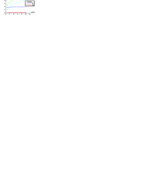
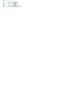
Figure 14: a) Cosine-shaped wavefunction of the electron on a $2$-dimensional square grid with the nuclear spins located at the vertex points, b) plot of the ratios $d_{1}=\frac{\tilde{\gamma}(\Delta M_{0})}{g_{2}}$ and $d_{2}=\frac{\tilde{\gamma}(\Delta S_{0})}{g_{2}}$ for a cosine and a Gaussian shaped wave function. For $N=10^{4}$, both ratios $d_{1}$ and $d_{2}$ are on the order of $10^{-4}$, together with c), we see that the dipolar interaction is negligible. c) plot of the ratios $d_{3}=\frac{\tilde{\gamma}(U^{\dagger}SU)_{00}}{g_{2}}$ and $d_{4}=\frac{\tilde{\gamma}(U^{\dagger}2MU)_{00}}{g_{2}}$ for a cosine and a Gaussian shaped wave function. For $N=10^{4}$, $d_{3}$ is on the order of $10^{-2}$ and $d_{4}$ is zero due to the symmetry of the electron wavefunction.

and $|c_{2}|^{2}=(\Delta S_{0})^{2}$ for the second term. $\Delta M_{0}$ and $\Delta S_{0}$ depend only on the electron wave function and the lattice geometry. To numerically calculate $\Delta M_{0}$ and $\Delta S_{0}$ and the effect of the last two terms in (7.1.1), we consider the case where the nuclei lie in a $2$-dimensional square plane with length $R=\sqrt{N}r_{0}$ of each side on a grid with equal spacings $r_{0}$ (=$0.24nm$ in GaAs [27])[see figure 14(a)]. Consequently, $\theta_{ij}=\pi/2$, which simplifies many expressions in $H_{dd}$. These assumptions can be made as the height of the QD is small compared to its diameter, so that the variation of $\theta$ that is dependent of the height of the QD is small, $\theta_{ij}\approx\pi/2$.

To illustrate our results we consider two simple choices for the electron wavefunction such that $\alpha_{l}^{(0)}=\frac{1}{\sum_{l}f_{1/2}(\mathbf{r}_{l})}f_{1/2}(\mathbf{r}_{l})$ with $\mathbf{r}_{l}=(x_{l},y_{l})$,

$$f_{1}(\mathbf{r}_{l})=\cos{\left(\frac{\pi}{2}\frac{x_{l}}{R}\right)}^{2}\cdot\cos{\left(\frac{\pi}{2}\frac{y_{l}}{R}\right)}^{2},$$ (4arasaybu)

and

$$f_{2}(\mathbf{r}_{l})=\exp{(-\sqrt{2}r_{l}^{2}/R^{2})}.$$ (4arasaybv)

To show that the direct dipolar interaction is a weak effect compared to the optical-nuclear coupling $g$, we calculate the ratios

$$d_{1}=\frac{\tilde{\gamma}(\Delta M_{0})}{g_{2}}=\frac{\tilde{\gamma}(\Delta M_{0})}{\frac{\Omega_{c}\Omega_{l}g_{n}}{8\Delta^{\prime}_{T_{-}}\tilde{\omega}_{e}}}=\frac{8\Delta^{\prime}_{T_{-}}\tilde{\omega}_{e}}{\Omega_{c}\Omega_{l}}\frac{\tilde{\gamma}}{A}\frac{(\Delta M_{0})}{\sqrt{\sum_{i=1}^{N}\alpha_{i}^{(0)2}}}.$$ (4arasaybw)

and $d_{2}=\frac{\tilde{\gamma}\Delta S_{0}}{g_{2}}$. For the parameters used for the simulation in Section 3, $\frac{8\Delta^{\prime}_{T_{-}}\tilde{\omega}_{e}}{\Omega_{c}\Omega_{l}}\frac{\tilde{\gamma}}{A}\approx 4\cdot 10^{-5}$ with $\tilde{\gamma}$ for GaAs [27]. A plot of $d_{1}$ and $d_{2}$ is shown in figure 14(b). $d_{1}$ and $d_{2}$ are both on the order of $10^{-4}-10^{-5}$, for $N>1000$ nuclear spins and increase slowly with $N$. The last two terms in (7.1.1), $(U^{\dagger}SU)_{00}b^{\dagger}_{0}b_{0}$ and $(U^{\dagger}2MU)_{00}b_{0}b_{0}$ are small and zero, respectively, as can be seen in figure 14(c): The ratio of $d_{3}=\frac{\tilde{\gamma}(U^{\dagger}SU)_{00}}{g_{2}}$ is on the order of $10^{-3}-10^{-2}$ for $N>1000$ nuclear spins and the ratio $d_{4}=\frac{\tilde{\gamma}(U^{\dagger}2MU)_{00}}{g_{2}}$ is zero due to the symmetry of the electron wavefunction in this setting. Shifting the electron wavefunction such that it is not longer symmetric with respect to the coordinate origin, $d_{4}$ is on the order of $10^{-4}$. We assume that the nuclei lie in a plane, so there is no displacement of $b_{0}$ as $D_{ij}=0$ for $\theta_{ij}=\frac{\pi}{2}$. Therefore, we have shown, that direct dipolar coupling is an effect that does not affect our protocol.

The hyperfine coupling between electron spin and nuclear spins leads to a mediated dipolar interaction between nuclear spins [61]. In the bosonic description, the electron couples solely to the $b_{0}$ mode, thus, the mediated coupling leads only to an energy shift

$$\frac{g_{n}^{2}}{4\tilde{\omega}_{e}}b^{\dagger}_{0}b_{0}$$ (4arasaybx)

that depends on the Zeeman splitting $\tilde{\omega}_{e}$ and the number of nuclear excitations. This was already present in (4h) and is not affecting the protocol, in fact it can help as Kurucz et al. [62] showed.

For spin-$1/2$ systems, as considered here, the quadrupolar interaction is not present. For large spin I (e.g. $3/2$ or $9/2$) nuclei present in GaAs, there is a significant quadrupolar term. Depending on the strain, up to $g_{q}\lesssim 10^{-2}\mu$eV have been measured [63]. Therefore, for $I>1/2$, dots with small strain have to be considered. The quadrupolar interaction [60] can be treated on a similar footing as the dipolar coupling in Section 7.1.1.

7.2 Errors in the bosonic picture

We have relied on a simple bosonic description of the collective nuclear excitations and neglected all corrections to that simplified picture. For homogeneous coupling ($\alpha_{j}=$const) this is the well-known Holstein-Primakoff approximation [33] and for systems cooled to a dark state [64] at moderate polarization ($\langle A^{z}\rangle$ on the order of $-1/2$) spin, replacing the collective spin operators by bosonic operators is accurate to $o(1/N)$. The generic inhomogeneous case is discussed in detail in [35]. In that case, the Hamiltonian (3) can be seen as a zeroth order approximation in a small parameter $\sim q(1-P)$, where $q\geq 1/2$ and $q=1/2$ for a homogeneous wave function. The first-order correction analyzed in [35] contains two contributions: (i) a polarization dependent scaling of the coupling-strength $g_{n}$ which has negligible effect on the adiabatic transfer we consider and (ii) an effective coupling of $b$ to bath modes due to the inhomogeneity of the $A^{z}$ term. This correction can be computed similarly to the one in the preceding subsections by rewriting $A^{z}$ in terms of bosonic operators. The coupling strength of the leading term is found to be $\sim A/N=g_{n}/\sqrt{N}$ and is thus much weaker than $g_{1/2}$. Since $g_{1/2}$ also characterizes the energy splitting between different excitation-manifolds in the JC system, this term is further suppressed by energy considerations.

8 Summary and Conclusions

We have shown how to realize a quantum interface between the polarized nuclear spin ensemble in a singly charged quantum dot and a traveling optical field. The coupling is mediated by the electron spin and the mode of a high-Q optical cavity to which the quantum dot is strongly coupled. Our proposal exploits the strong hyperfine and cavity coupling of the electron to eliminate the electronic degree of freedom and obtain an effective coupling between cavity and nuclei. First, we have studied several possibilities to directly map the state of the cavity to the nuclei and discussed error processes and drawbacks of these schemes. Then, we have presented a more sophisticated interface which is robust to cavity decay. Read-out is achieved via cavity decay while write-in is based on the generation of two-mode squeezed states of nuclei and output field and teleportation. For typical values of hyperfine interaction and cavity lifetimes, several ebit of entanglement can be generated before internal nuclear dynamics becomes non-negligible. All proposed schemes take advantage of the bosonic character of the nuclear system at high polarization, which implies that all the relevant dynamics of nuclei, cavity and output field is described by quadratic interactions. This allows the analytical solution of the dynamics and a detailed analysis of the entanglement generated. We show that apart from mapping a light state to the nuclei, the couplings described enable the preparation of arbitrary Gaussian states of the nuclear mode.

For highly polarized nuclear spin systems the bosonic description provides a very convenient framework for the discussion of (dipolar and quadrupolar) “internal” nuclear dynamics. It is seen that these processes do not appreciably affect the performance of the interface.

Our results give further evidence that nuclear spins in quantum dots can be a useful system for quantum information processing. In view of the recent impressive experimental progress in both dynamical nuclear polarization of quantum dots and quantum dot cavity-QED, their use for QIP protocols may not be too far off.

9 Acknowledgements

This work was supported by the DFG within SFB 631 and the Excellence Cluster NIM.

Appendix A Gaussian states and operations

Gaussian states and operations play a central role in quantum information with continuous variable systems [65]. To make this work self-contained we briefly summarize here the main properties of Gaussian states and operations with particular regard to their entanglement.

Gaussian states are a family of states occurring very frequently in quantum optics, e.g., in the form of coherent, squeezed, and thermal states. Despite being defined on an infinite dimensional Hilbert space [${\cal F}_{+}(\mathbbm{R}^{2N})$, the symmetric Fock space over $\mathbbm{R}^{2N}$] they are characterized by a finite number of real parameters, namely the first and second moments of $N$ pairs of canonically conjugate observables $(Q_{1},P_{1},\dots,Q_{N},P_{N})\equiv\vec{R}$.

One way to define them is that their characteristic function, i.e., the expectation values $\chi(\xi)=\mathrm{tr}(W_{\xi}\rho)$ of the displacement operators $W_{\xi}=\exp(i\xi^{T}\vec{R}),\xi\in\mathbbm{R}^{2N}$ is a Gaussian function [66]:

$$\chi(\rho)=\exp(-i\xi^{T}d-1/4\xi^{T}\gamma\xi).$$ (4arasayby)

The displacement vector $d\in\mathbbm{R}^{2N}$ and the $2N\times 2N$ real positive covariance matrix (CM) $\gamma$ are given by the expectations and (co)variances of the $R_{k}$:

$$d_{k} = \mathrm{tr}[\rho R_{k}],$$ (4arasaybza)

$$\gamma_{kl} = \langle R_{i}R_{j}+R_{j}R_{i}\rangle-2\langle R_{i}\rangle\langle R_{j}\rangle.$$ (4arasaybzb)

All $d\in\mathbbm{R}^{2N}$ are admissible displacement vectors and any real positive matrix $\gamma$ is a valid CM if it satisfies $\gamma\geq i\sigma_{N}$ when the symplectic matrix $\sigma_{N}$ is

$$\sigma_{N}=\oplus_{l=1}^{N}\sigma_{1}\,\,\,\mathrm{with}\,\,\,\sigma_{1}=\left(\begin{array}[]{cc}0&-1\\ 1&0\end{array}\right).$$ (4arasaybzca)

The last condition summarizes all the uncertainty relations for the canonical operators $R_{j}$. These operators are related to the creation and annihilation operators $a^{\dagger}_{j},a_{j}$ by the relations $Q_{j}=(a_{j}+a_{j}^{\dagger})/\sqrt{2}$ and $P_{j}=-i(a_{j}-a_{j}^{\dagger})/\sqrt{2}$.

An example for a one-mode Gaussian state is a coherent state $\left|\alpha\right>$, with covariance matrix $\gamma=\mathbbm{1}$ and displacement $d=(\mathrm{Re}|\alpha|,\mathrm{Im}|\alpha|)/\sqrt{2}$.

Entanglement: All information about the entanglement properties of Gaussian states is encoded in the CM. Given a CM, there are efficient criteria to decide whether a Gaussian state is entangled or not.

To apply these criteria, it is useful to write the CM of a bipartite $N\times M$ Gaussian states in the following form,

$$\gamma=\left(\begin{array}[]{cc}A&C\\ C^{T}&B\end{array}\right),$$ (4arasaybzcd)

where the $2N\times 2N$ ($2M\times 2M$) matrix $A$ ($B$) refers to the covariances of the quadrature operators associated with the first (second) system and $C$ contains the covariances between the two systems. $A$ ($B$) are the CM of the reduced state in the first (second) system only.

In the case of a two-mode system the criteria [67, 68] are necessary and sufficient for separability: a state with CM $\gamma$ is entangled if and only if $\det\gamma+1-\det A-\det B+2\det C\not\geq 0$. In this case, entanglement is necessarily accompanied by a non-positive partial transpose (npt) [69]. For more modes, entangled states with positive partial transpose exist [70] and more general criteria to decide entanglement have to be used [71, 72].

For pure states, the analysis of entanglement properties becomes particularly easy since all such states can be transformed to a simple standard form, namely a collection of two-mode squeezed states (TMSS) and vacuum states, by local unitaries [73], hence the entanglement of such a state is fully characterized by the vector of two-mode squeezing parameters. This also shows that for a $1\times M$ system in a pure state one can always identify a single mode such that only it (and not the $M-1$ other modes) is entangled with the first system.

For many Gaussian states it is also possible to make quantitative statements about the entanglement, i.e. to compute certain entanglement measures. For pure $N\times M$ states, the entropy of entanglement can be computed from the symplectic eigenvalues of the reduced CM $A$ (or, equivalently, $B$). These are given by the modulus of the eigenvalues of $\sigma_{N}A$ [74]. All symplectic eigenvalue $\lambda\geq 1$ corresponds to a TMSS with squeezing parameter $\mathrm{arccosh}(\lambda)/2$ in the standard form of the state at hand and contributes $\lambda^{2}\log_{2}\lambda^{2}-(\lambda-1)^{2}\log_{2}(\lambda^{2}-1)$ to the entanglement entropy of the system.
For mixed states, it is possible to compute the negativity [74] for any $N\times M$ system from the symplectic eigenvalues of the CM of the partially transposed state (which is related to the CM obtained by replacing all momenta $P_{j}$ in the second system by $-P_{j}$). Every symplectic eigenvalue $\lambda<1$ contributes $-\log_{2}\lambda$ to the negativity.
For $1\times 1$ Gaussian states with $\det A=\det B$ (so-called symmetric states), the entanglement of formation (EoF) can be computed [75] and for more general states a Gaussian version of EoF is available [43]. Even if the states are not certain to be Gaussian, several of the Gaussian quantities can serve as lower bounds for the actual amount of entanglement [76].

Gaussian operations: Operations that preserve the Gaussian character of the states they act on are called Gaussian operations [57]. Like the Gaussian states they are only a small family (in the set of all operations) but play a prominent role in quantum optics, since they comprise many of the most readily implemented state transformations and dynamics. With Gaussian operations and Gaussian states many of the standard protocols of quantum information processing such as entanglement generation, quantum cryptography, quantum error correction and quantum teleportation can be realized [65].

Of particular interest for us are the Gaussian unitaries, i.e. unitary evolutions generated by Hamiltonians that are at most quadratic in the creation and annihilation operators. Unitary displacements $W_{\xi}$ are generated by the linear Hamiltonian $\xi^{T}\vec{R}$. All other Gaussian unitaries can be composed of three kinds [77], named according to their optical incarnations. The phase shifter ($H=a^{\dagger}a$) corresponds to the free evolution of an harmonic system. The beam splitter ($H=ab^{\dagger}+a^{\dagger}b$) couples two modes. Both generators do not change the total photon number and are therefore examples of passive transformations. The remaining type of Gaussian unitary is active: the (single-mode) squeezer is generated by the squeezing Hamiltonian $H=a^{2}+(a^{\dagger})^{2}$, which, when acting on the vacuum state decreases the variance in one quadrature ($Q$) by a factor $f<1$ and increases the other one by $1/f$. Combining these building blocks in the proper way, all other unitaries generated by quadratic Hamiltonians, e.g. the two-mode squeezing transformation ($H=ab+a^{\dagger}b^{\dagger}$) can be obtained.

Both active and passive transformations map field operators to a linear combination of field operators (disregarding displacements caused by linear parts in the Hamiltonians, which can always be undone by a further displacement), i.e. for all Gaussian unitaries we have in the Heisenberg picture

$$U\vec{R}U^{\dagger}=S\vec{R}\equiv\vec{R}^{\prime}.$$ (4arasaybzce)

Here $S$ is a symplectic map on $\mathbbm{R}^{2N}$, i.e. $S$ preserves the symplectic matrix $\sigma_{N}$, assuring that $R_{i}$ and $R_{i}^{\prime}$ satisfy the same commutation relations. We denote by $U_{S}$ the unitary corresponding to the symplectic transformation $S$. Passive operations correspond to symplectic transformations that are also orthogonal.

In the Schrödinger picture, $U_{S}$ transforms the Gaussian state with CM $\gamma$ and displacement $d$ such that $(\gamma,d)\mapsto(S\gamma S^{T},Sd)$. The two-mode squeezing transformations

$$T(r)=\left(\begin{array}[]{cc}\cosh{(r)}\mathbbm{1}&\sinh{(r)}\sigma_{x}\cr\sinh{(r)}\sigma_{x}&\cosh{(r)}\mathbbm{1}\end{array}\right)$$ (4arasaybzcf)

used in Sec. 4.1 is an important example of a active symplectic transformation.

Besides Gaussian unitaries, Gaussian measurements are another important and readily available tool. Gaussian measurements are generalized measurements represented by a positive-operator-valued measure $\left\{\left|\gamma,d\right>\left<\gamma,d\right|{\gamma,d},d\in\mathbbm{R}^{2N}\right\}$ that is formed by all the projectors obtained from a pure Gaussian state $\left|\gamma,0\right>\left<\gamma,0\right|{\gamma,0}$ by displacements. The most important example is a limiting case of the above: the quadrature measurements (von Neumann measurements which project on the (improper, infinitely squeezed) eigenstates of, e.g., $Q$). In quantum optics, these are well approximated by homodyne detection. For example, the “Bell- or “EPR-measurement” that is part of the teleportation protocol is a measurement of the commuting quadrature operators $Q_{1}+Q_{2}$ and $P_{1}-P_{2}$.

Appendix B Landau-Zener transitions

In a rotating frame with $U=\exp{[-\frac{i}{2}\int(\omega_{1}-\omega_{2})\sigma_{z}+(\omega_{1}+\omega_{2})\mathbbm{1}\,\mathrm{dt}]}$ the Heisenberg equations, given by (4l), read:

$$\dot{u^{\prime}}= -ig\exp{\left(i\int(\omega_{1}-\omega_{2})\mathrm{dt}\right)}v^{\prime}$$ (4arasaybzcg)

$$\dot{v^{\prime}}= -ig\exp{\left({-i\int(\omega_{1}-\omega_{2})}\mathrm{dt}\right)}u^{\prime}$$ (4arasaybzch)

The initial boundary conditions of the coupled differential Equations (4arasaybzcg) and (4arasaybzch) are now chosen such, that the photon operator $a$ at time $t\rightarrow-\infty$ is mapped to the nuclear spin operator $b$ at $t\rightarrow\infty$

$$u^{\prime}_{-\infty}=1,|v^{\prime}_{-\infty}|=0.$$ (4arasaybzci)

Eliminating $u^{\prime}$ in (4arasaybzcg) and (4arasaybzch) leads to the single equation:

$$\ddot{v^{\prime}}+i\beta t\dot{v^{\prime}}+g^{2}v^{\prime}=0,$$ (4arasaybzcj)

where $\dot{g}=0$. Together with the substitution $v^{\prime}=e^{-\frac{i}{2}\int(\omega_{1}-\omega_{2})dt}U_{1}$, (4arasaybzcj) reduces to the so called Weber equation:

$$\ddot{U_{1}}+\left(g^{2}-i\frac{\beta}{2}+\frac{\beta^{2}}{4}t^{2}\right)U_{1}=0.$$ (4arasaybzck)

Solving (4arasaybzck) as proposed by Landau and Zener and considering the asymptotic behavior of the solution at $t\rightarrow\infty$, it is found to be

$$\lim_{t\to\infty}U_{1}(t)=-K\frac{\sqrt{2\pi}}{\Gamma(i\gamma_{z}+1)}e^{-\frac{1}{4}\pi\gamma_{z}}e^{i\beta t^{2}}(\sqrt{\beta}t)^{i\gamma_{z}},$$ (4arasaybzcl)

where $\gamma_{z}=\frac{g_{1}^{2}}{\beta}$ and the constant $K=\sqrt{\gamma_{z}}\exp{\left(-\frac{\gamma_{z}\pi}{4}\right)}$. The probability that the photonic operator $a$ is mapped to the collective nuclear spin operator $b$ is given by (4o).

References

- [1] D. P. DiVincenzo. The physical implementation of quantum computation. Fort. Phys., 48:771, 2000.
- [2] P. Zoller et al. Quantum information processing and communication. Eur. Phys. J. D, 36:203, 2005.
- [3] J. I. Cirac, P. Zoller, H. J. Kimble, and H. Mabuchi. Quantum state transfer and entanglement distribution among distant nodes in a quantum network. Phys. Rev. Lett., 78:3221, 1997.
- [4] A. E. Kozekhin, K. Mølmer, and E. S. Polzik. Quantum memory for light. Phys. Rev. A, 62:033809, 2000.
- [5] M. Fleischhauer and M. D. Lukin. Quantum memory for photons: Dark state polaritons. Phys. Rev. A, 65:022314, 2002.
- [6] X. Maître, E. Hagley, G. Nogues, C. Wunderlich, P. Goy, M. Brune, J. M. Raimond, and S. Haroche. Quantum memory with a single photon in a cavity. Phys. Rev. Lett., 79:769, 1997.
- [7] B. Julsgaard, J. Sherson, J. I. Cirac, J. Fiurášek, and E. S. Polzik. Experimental demonstration of quantum memory for light. Nature, 432:482, 2004.
- [8] T. Wilk, S. C. Webster, A. Kuhn, and G. Rempe. Single-Atom Single-Photon Quantum Interface. Science, 317(5837):488–490, 2007.
- [9] W. Rosenfeld, S. Berner, J. Volz, M. Weber, and H. Weinfurter. Remote preparation of an atomic quantum memory. Phys. Rev. Lett., 98:050504, 2007.
- [10] K. S. Choi, H. Deng, J. Laurat, and H. J. Kimble. Mapping photonic entanglement into and out of a quantum memory. Nature, 452:67, 2008.
- [11] B. B. Blinov, D. L. Moehring, L.-M. Duan, and C. Monroe. Observation of entanglement between a single trapped atom and a single photon. Nature, 428:153, 2004.
- [12] D. Loss and D. P. DiVincenzo. Quantum computation with quantum dots. Phys. Rev. A, 57:120, 1998.
- [13] A. Imamoğlu, D. D. Awschalom, G. Burkard, D. P. DiVincenzo, D. Loss, M. Sherwin, and A. Small. Quantum information processing using quantum dot spins and cavity-qed. Phys. Rev. Lett., 83:4204, 1999.
- [14] R. Hanson and D. D. Awschalom. Coherent manipulation of single spins in semiconductors. Nature, 453:1043, 2008.
- [15] W. Yao, R.-B. Liu, and L. J. Sham. Theory of control of the spin-photon interface for quantum networks. Phys. Rev. Lett., 95:030504, 2005.
- [16] J. P. Reithmaier, G. Sek, A. Loffler, C. Hofmann, S. Kuhn, S. Reitzenstein, L. V. Keldysh, V. D. Kulakovskii, T. L. Reinecke, and A. Forchel. Strong coupling in a single quantum dot-semiconductor microcavity system. Nature, 432:197, 2004.
- [17] T. Yoshie, A. Scherer, J. Hendrickson, G. Khitrova, H. M. Gibbs, G. Rupper, C. Ell, O. B. Shchekin, and D. G. Deppe. Vacuum Rabi splitting with a single quantum dot in a photonic crystal nanocavity. Nature, 432:200, 2004.
- [18] K. Hennessy, A. Badolato, M. Winger, D. Gerace, M. Atature, S. Gulde, S. Fält, E. L. Hu, and A. Imamoğlu. Quantum nature of a strongly coupled single quantum dot-cavity system. Nature, 445:896, 2007.
- [19] J. P. Reithmaier. Strong exciton–photon coupling in semiconductor quantum dot systems. Semiconductor Science and Technology, 23:123001, 2008.
- [20] J. M. Taylor, A. Imamoğlu, and M. D. Lukin. Controlling a mesoscopic spin environment by quantum bit manipulation. Phys. Rev. Lett., 91:246802, 2003.
- [21] J. M. Taylor, G. Giedke, H. Christ, B. Paredes, J. I. Cirac, P. Zoller, M. D. Lukin, and A. Imamoğlu. Quantum information processing using localized ensembles of nuclear spins. arXiv:cond-mat/0407640, 2004.
- [22] L. Landau. Zur theorie der energieübertragung bei stößen. Physikalische Zeitschrift der Sowjetunion, 1:88, 1932.
- [23] C. Zener. Non-adiabatic crossing of energy levels. Proc. Roy. Soc. Lond. A, 137:696, 1932.
- [24] K. Bergmann, H. Theuer, and B. W. Shore. Coherent population transfer among quantum states of atoms and molecules. Rev. Mod. Phys., 70:1003, 1998.
- [25] H. Schwager, J. I. Cirac, and G. Giedke. A quantum interface between light and nuclear spins in quantum dots. arXiv:0810.4488v2 [cond-mat.mes-hall], 2008.
- [26] S. L. Braunstein and H. J. Kimble. Teleportation of continuous quantum variables. Phys. Rev. Lett., 80:869, 1998.
- [27] J. Schliemann, A. Khaetskii, and D. Loss. Electron spin dynamics in quantum dots and related nanostructures due to hyperfine interaction with nuclei. J. Phys: Cond. Mat., 15:R1809, 2003.
- [28] A. S. Bracker, E. A. Stinaff, D. Gammon, M. E. Ware, J. G. Tischler, A. Shabaev, A. L. Efros, D. Park, D. Gershoni, V. L. Korenev, and I. A. Merkulov. Optical pumping of electronic and nuclear spin in single charge-tunable quantum dots. Phys. Rev. Lett., 94:047402, 2005.
- [29] P. Maletinsky, A. Badolato, and A. Imamoğlu. Dynamics of quantum dot nuclear spin polarization controlled by a single electron. Phys. Rev. Lett., 99:056804, 2007.
- [30] J. Skiba-Szymanska, A. V. Nikolaenko, M. N. Makhonin, I. Drouzas, M. S. Skolnick, A. B. Krysa, and A. I. Tartakovskii. Strong Overhauser effect in individual InP/GaInP dots. Phys. Rev. B, 77:165338, 2008.
- [31] B. Urbaszek, P.-F. Braun, X. Marie, O. Krebs, A. Lemaitre, P. Voisin, and T. Amand. Efficient dynamical nuclear polarization in quantum dots: Temperature dependence. Phys. Rev. B, 76:201301(R), 2007.
- [32] P. Maletinsky. PhD thesis, ETH Zürich, http://e-collection.ethbib.ethz.ch/view/eth:30788, 2008.
- [33] T. Holstein and H. Primakoff. Field dependence of the intrinsic domain magnetization of ferromagnet. Phys. Rev., 58:1098, 1940.
- [34] H. Christ, J. I. Cirac, and G. Giedke. Nuclear spin polarization in quantum dots-the homogeneous limit. Solid State Sciences, 2007.
- [35] H. Christ. Quantum Computation with Nuclear Spins in Quantum Dots. PhD thesis, TU München, http://mediatum2.ub.tum.de/doc/635960/635960.pdf, 2008.
- [36] E. Brion, L. H. Pedersen, and K. Mølmer. Adiabatic elimination in a lambda system. arXiv:quant-ph/0610056, 2006.
- [37] X. Xu, Y. Wu, B. Sun, Q. Huang, J. Cheng, D. G. Steel, A. S. Bracker, D. Gammon, C. Emary, and L. J. Sham. Fast spin state initialization in a singly charged inas-gaas quantum dot by optical cooling. Phys. Rev. Lett., 99:097401, 2007.
- [38] M. O. Scully and M. S. Zubairy. Quantum Optics. Cambridge University Press, 1997.
- [39] K. Hammerer, M. M. Wolf, E. S. Polzik, and J. I. Cirac. Quantum benchmark for storage and transmission of coherent states. Phys. Rev. Lett., 94:150503, 2005.
- [40] A. Furusawa, J. L. Sørensen, S. L. Braunstein, C. A. Fuchs, H. J. Kimble, and E. S. Polzik. Unconditional quantum teleportation. Science, 282:706, 1998.
- [41] C. M. Caves. Quantum limits on noise in linear amplifiers. Phys. Rev. D, 26:1817, 1982.
- [42] H. Scutaru. Transition probabilities for quasifree states. J. Math. Phys., 39:6403, 1998.
- [43] M. M. Wolf, G. Giedke, O. Krüger, R. F. Werner, and J. I. Cirac. Gaussian entanglement of formation. Phys. Rev. A, 69:052320, 2003.
- [44] A. S. Parkins, P. Marte, P. Zoller, O. Carnal, and H. J. Kimble. Quantum-state mapping between multilevel atoms and cavity light fields. Phys. Rev. A, 51:1578, 1995.
- [45] Y. Takahashi, H. Hagino, Y. Tanaka, B.-S. Song, T. Asano, and S. Noda. High-q nanocavity with a 2-ns photon lifetime. Opt. Express, 15(25):17206–17213, 2007.
- [46] A. Messiah. Quantenmechanik Band 2. de Gruyter, 1985.
- [47] Y. Shi and Y.-S. Wu. Perturbative formulation and nonadiabatic corrections in adiabatic quantum-computing schemes. Phys. Rev. A, 69:024301, 2004.
- [48] S. Clark, A. Peng, M. Gu, and S. Parkins. Unconditional preparation of entanglement between atoms in cascaded optical cavities. Phys. Rev. Lett., 91:177901, 2003.
- [49] B. Kraus and J. I. Cirac. Discrete entanglement distribution with squeezed light. Phys. Rev. Lett., 92:013602, 2004.
- [50] M. G. A. Paris. Displacement operator by beam splitter. Phys. Lett. A, 217:78, 1996.
- [51] C. W. Gardiner and P. Zoller. Quantum Noise. Springer Verlag, Berlin, 2nd edition, 2000.
- [52] J. Williamson. American Journal of Mathematics, 58:141, 1936.
- [53] M. B. Plenio. Logarithmic negativity: A full entanglement monotone that is not convex. Phys. Rev. Lett., 95:090503, 2005.
- [54] C. H. Bennett, H. J. Bernstein, S. Popescu, and B. Schumacher. Concentrating partial entanglement by local operations. Phys. Rev. A, 53:2046, 1996.
- [55] L. Vaidman. Teleportation of quantum states. Phys. Rev. A, 49:1473, 1994.
- [56] J. Fiurášek. Improving the fidelity of continuous-variable teleportation via local operations. Phys. Rev. A, 66:012304, 2002.
- [57] G. Giedke and J. I. Cirac. The characterization of Gaussian operations and distillation of Gaussian states. Phys. Rev. A, 66:032316, 2002.
- [58] B. Kraus, K. Hammerer, G. Giedke, and J. I. Cirac. Entanglement generation and hamiltonian simulation in continuous-variable systems. Phys. Rev. A, 67:042314, 2002.
- [59] Z. Kurucz, M. W. Sørensen, J. M. Taylor, M. D. Lukin, and M. Fleischhauer. Qubit protection in nuclear-spin quantum dot memories. Phys. Rev. Lett., 103:010502, 2009.
- [60] C. P. Slichter. Principles of Magnetic Resonance. Springer Verlag, Berlin, 1990.
- [61] W. Yao, R.-B. Liu, and L. J. Sham. Theory of electron spin decoherence by interacting nuclear spins in a quantum dot. Phys. Rev. B, 74:195301, 2006.
- [62] Z. Kurucz and M. Fleischhauer. Continuous-variable versus electromagnetically-induced-transparency-based quantum memories. Phys. Rev. A, 78:023805, 2008.
- [63] P. Maletinsky, M. Kroner, and A. Imamoğlu. Demagnetization of quantum dot nuclear spins: Breakdown of the nuclear spin temperature approach. unpublished, 2008.
- [64] A. Imamoğlu, E. Knill, L. Tian, and P. Zoller. Optical pumping of quantum-dot nuclear spins. Phys. Rev. Lett., 91:017402, 2003.
- [65] S. L. Braunstein and P. van Loock. Quantum information with continuous variables. Rev. Mod. Phys., 77:513, 2005.
- [66] J. Manuceau and A. Verbeure. Quasi-free states of the C.C.R.–Algebra and Bogoliubov transformations. Comm. Math. Phys., 9:293, 1968.
- [67] L.-M. Duan, G. Giedke, J.I. Cirac, and P. Zoller. Physical implementation for entanglement purification of Gaussian continuous-variable quantum states. Phys. Rev. A, 62:032304, 2000.
- [68] R. Simon. Peres-Horodecki separability criterion for continuous variable systems. Phys. Rev. Lett., 84:2726, 2000.
- [69] A. Peres. Separability criterion for density matrices. Phys. Rev. Lett., 77:1413, 1996.
- [70] R. F. Werner and M. M. Wolf. Bound entangled Gaussian states. Phys. Rev. Lett., 86:3658, 2001.
- [71] G. Giedke, B. Kraus, M. Lewenstein, and J. I. Cirac. Separability properties of three-mode Gaussian states. Phys. Rev. A, 64:052303, 2001.
- [72] P. Hyllus and J. Eisert. Optimal entanglement witnesses for continuous-variable systems. N. J. Phys., 8:51, 2006.
- [73] G. Giedke, J. Eisert, J. I. Cirac, and M. B. Plenio. Entanglement transformations of pure gaussian states. J. Quant. Inf. Comp., 3(3):211, 2003.
- [74] G. Vidal and R. F. Werner. A computable measure of entanglement. Phys. Rev. A, 65:032314, 2002.
- [75] G. Giedke, M. M. Wolf, O. Krüger, R. F. Werner, and J. I. Cirac. Entanglement of formation for Gaussian states. Phys. Rev. Lett., 91:107901, 2003.
- [76] M. M. Wolf, G. Giedke, and J. I. Cirac. Extremality of Gaussian quantum states. Phys. Rev. Lett., 96:080502, 2006.
- [77] S. L. Braunstein. Squeezing as an irreducible resource. Phys. Rev. A, 71(5):055801, 2005.