A note on the holography of
Chern-Simons matter theories with flavour

Stefan Hohenegger and Ingo Kirsch^a

^a Institut für Theoretische Physik, ETH Zürich

CH-8093 Zürich, Switzerland

Abstract

We study a three-dimensional $\mathcal{N}=3$ $U(N)_{k}\times U(N)_{-k}$ Chern-Simons matter theory with flavour, corresponding to the $\mathcal{N}=6$ Aharony-Bergman-Jafferis-Maldacena CSM theory coupled to $2N_{f}$ fundamental fields. The dual holographic description is given by the near-horizon geometry of $N$ M2-branes at a particular hypertoric geometry ${\cal M}_{8}$. We explicitly construct the space ${\cal M}_{8}$ and match its isometries to the global symmetries of the field theory. We also discuss the model in the quenched approximation by embedding probe D6-branes in $AdS_{4}\times{\mathbb{CP}^{3}}$.

1 Introduction

Recently, there has been a renewed interest in three-dimensional superconformal Chern-Simons-matter (CSM) theories. Other than their purely topological cousins, this type of Chern-Simons theories exhibits non-trivial dynamics due to the coupling to matter fields. Bagger and Lambert [1] as well as Gustavsson [2] (BLG) constructed a three-dimensional $\mathcal{N}=8$ superconformal Chern-Simons gauge theory with manifest $SO(8)$ R-symmetry. A unitary realization of the involved three-algebra restricted the gauge group to $SO(4)$. After the reformulation of the BLG theory as a $SU(2)\times SU(2)$ CSM theory [3], Aharony, Bergman, Jafferis and Maldacena (ABJM) [4] constructed a $\mathcal{N}=6$ CSM theory with gauge group $U(N)\times U(N)$ at level $k$ as the world-volume theory of $N$ M2-branes at a $\mathbb{C}^{4}/\mathbb{Z}_{k}$ orbifold.

A prerequisite for making the above theory interesting for more realistic applications, e.g. in condensed matter physics, is the introduction of light matter fields in the fundamental representation of the gauge group. The fundamentals could serve, for instance, as a prototype for strongly-coupled electrons. First steps in this direction have been taken in [5, 6, 7], which discussed $\mathcal{N}=2$ supersymmetric CSM theories with fundamental matter and discovered an interesting strong-weak coupling Seiberg-type duality. However, Refs. [5, 6, 7] have not yet addressed a possible holographic description of CSM theories with flavour, which over the last years has turned out to be remarkably successful for Yang-Mills theories (see e.g. [8] for a review).

In this note we fill this gap by proposing a holographic description of the ABJM model coupled to $2N_{f}$ light fundamental fields. We show that the field theory, whose action will be written using $\mathcal{N}=2$ superspace formalism, preserves $\mathcal{N}=3$ supersymmetry for particular values of the coupling constants. We find that other than in the (unflavoured) ABJM model, where supersymmetry is enhanced to $\mathcal{N}=6$ [4], the supersymmetry of the present model remains $\mathcal{N}=3$ in the infrared. The latter describes the low-energy region of the open-string sector of the web-deformed type IIB configuration studied in [4] with two additional stacks of $N_{f}$ D5-branes. The T-dual type IIA setup, now involving $2N_{f}$ D6-branes, lifts to $N$ M2-branes at the origin of a toric hyperkähler geometry ${\cal M}_{8}$. We explicitly construct ${\cal M}_{8}$ and compare its isometry group to the global symmetries of the dual $\mathcal{N}=3$ field theory.

The corresponding near-horizon geometry includes the information of the (uplifted) flavour D6-branes and therefore their backreaction on the geometry. However, the complicated structure of the near-horizon metric impedes further progress along these lines. We therefore continue to discuss flavours in the quenched approximation, using holographic methods as initiated in [9, 10, 11]. This requires the embedding of probe D6-branes in $AdS_{4}\times{\mathbb{CP}^{3}}$, which is the near-horizon geometry of the ABJM setup in type-IIA string theory [4]. The D6-branes fill the $AdS_{4}$ space and wrap around a special Lagrangian submanifold inside the ${\mathbb{CP}^{3}}$. We show that the real projective space $\mathbb{R}\mathbb{P}^{3}$ is such a submanifold inside the ${\mathbb{CP}^{3}}$, and thus the corresponding embedding of the D6-branes is stable and supersymmetric.

The paper is organized as follows. In section 2 we present the $\mathcal{N}=3$ Chern-Simons Yang-Mills theory with matter in the fundamental representation of the $U(N)_{k}\times U(N)_{-k}$ gauge group. In section 3 we discuss the corresponding brane setup in type IIB string theory, its lift to $M$-theory and the corresponding near-horizon geometry. In section 4 we discuss the embedding of probe D6-branes in $AdS_{4}\times\mathbb{C}\mathbb{P}^{3}$.

Note added: After publication of the first version of this work, two further papers [12, 13] appeared in the arXiv, which have considerable overlap with the present work. In particular, taking into account a comment in the introduction of [12], we clarified the discussion of our brane-setup in section 3.

2 Chern-Simons Yang-Mills theory with fundamental matter

In this section we study a three-dimensional $\mathcal{N}=3$ superconformal $U(N)\times U(N)$ Chern-Simons-matter theory with flavour in the fundamental representation of the gauge group. This theory will be obtained by coupling $N_{f}$ fundamental hypermultiplets to the ABJM theory [4].

2.1 The action

The ABJM theory has gauge group $U(N)_{k}\times U(N)_{-k}$ and its action can be written in manifest $\mathcal{N}=2$ language [4]. Let us briefly review its field content. There are two bifundamental $\mathcal{N}=4$ hypermultiplets $(A,B^{\dagger})_{1,2}$ and two adjoint $\mathcal{N}=4$ vector multiplets consisting of the $\mathcal{N}=2$ vector fields $V_{1,2}$ and the chiral fields $\Phi_{1,2}$. Formally, there are also $k$ chiral multiplets ($q_{1,2}$) in the fundamental and $k$ chiral multiplets ($\tilde{q}_{1,2}$) in the anti-fundamental representation of each gauge group. These are assumed to be massive and, when integrated out, produce a Chern-Simons term via the parity anomaly. Thus at low energies all fundamental fields are integrated out, leaving only fields in the adjoint or bifundamental representation. In order to also have massless fundamental fields in the far infrared, we introduce $2N_{f}$ fundamental hypermultiplets $(Q^{r},\tilde{Q}^{r}{}^{\dagger})_{1,2}$ with $r=1,...,N_{f}$. The $\mathcal{N}=2$ superfields and their quantum numbers are summarized in the upper part of table 1.

	$U(N)$	$U(N)$	$U(k)$	$U(k)$	$U(N_{f})$	$U(N_{f})$	$\Delta$
$A_{1}$ , $A_{2}$	$N$	$\overline{N}$	1	1	1	1	$\frac{1}{2}$
$B_{1}$, $B_{2}$	$\overline{N}$	$N$	1	1	1	1	$\frac{1}{2}$
$\Phi_{1}$, $V_{1}$	adjoint	1	1	1	1	1	$1,0$
$\Phi_{2}$, $V_{2}$	1	adjoint	1	1	1	1	$1,0$
$q_{1}$	$N$	1	1	$\overline{k}$	1	1	$\frac{1}{2}$
$\tilde{q}_{1}$	$\overline{N}$	1	$k$	1	1	1	$\frac{1}{2}$
$q_{2}$	1	$N$	$\overline{k}$	1	1	1	$\frac{1}{2}$
$\tilde{q}_{2}$	1	$\overline{N}$	1	$k$	1	1	$\frac{1}{2}$
$Q_{1}$ , $\tilde{Q}_{1}^{\dagger}$	$N$	1	1	1	$N_{f}$	1	$\frac{1}{2}$
$Q_{2}$, $\tilde{Q}_{2}^{\dagger}$	1	$N$	1	1	1	$N_{f}$	$\frac{1}{2}$

Table 1: $\mathcal{N}=2,d=3$ superfields in the field theory.

In $\mathcal{N}=2$ superspace, the action can be written as a sum of three terms ${\cal S}={\cal S}_{\text{mat}}+{\cal S}_{\text{CS}}+{\cal S}_{\text{pot}}$, a matter part, a Chern-Simons part and a superpotential given by

$${\cal S}_{\text{mat}} =\int d^{3}xd^{4}\theta{\,\rm Tr}\left(-\bar{A}_{i}e^{-V_{1}}A_{i}e^{V_{2}}-\bar{B}_{i}e^{-V_{2}}B_{i}e^{V_{1}}\right)-\bar{Q}^{r}_{i}e^{-V_{i}}Q^{r}_{i}-{\tilde{Q}}^{r}_{i}e^{V_{i}}\bar{\tilde{Q}}^{r}_{i}\,,$$ (2.1)

$${\cal S}_{\text{CS}} =-i\frac{k}{4\pi}\int d^{3}xd^{4}\theta\int_{0}^{1}dt{\,\rm Tr}\left(V_{1}\bar{D}^{\alpha}(e^{tV_{1}}D_{\alpha}e^{-tV_{1}})-V_{2}\bar{D}^{\alpha}(e^{tV_{2}}D_{\alpha}e^{-tV_{2}})\right)\,,$$ (2.2)

$${\cal S}_{\text{pot}} =\int d^{3}xd^{2}\theta\,\left(W_{\text{ABJM}}+W_{\text{flavour}}\right)+c.c.\,,$$ (2.3)

where

$$W_{\text{ABJM}}=-\frac{k}{8\pi}{\,\rm Tr\,}(\Phi_{1}^{2}-\Phi_{2}^{2})+{\,\rm Tr\,}(B_{i}\Phi_{1}A_{i})+{\,\rm Tr\,}(A_{i}\Phi_{2}B_{i})$$ (2.4)

and

$$W_{\text{flavour}}=\alpha_{1}\tilde{Q}^{r}_{1}\Phi_{1}Q^{r}_{1}+\alpha_{2}\tilde{Q}^{r}_{2}\Phi_{2}Q^{r}_{2}\,.$$ (2.5)

The first term in the ABJM superpotential $W_{\text{ABJM}}$ [4] involving $\Phi^{2}_{1}$ and $\Phi^{2}_{2}$ is the $\mathcal{N}=3$ supersymmetry completion of the Chern-Simons action ${\cal S}_{\text{CS}}$, while the remaining two terms include the coupling to the bifundamentals $A_{1,2}$ and $B_{1,2}$. The superpotential $W_{\text{flavour}}$ describes the coupling of the new flavour fields $\tilde{Q}^{r}_{1,2},Q^{r}_{1,2}$ to the adjoints $\Phi_{1,2}$. The action preserves $\mathcal{N}=2$ supersymmetry for arbitrary values of the coupling constants $\alpha_{1,2}$.

There are no kinetic terms for the fields of the $\mathcal{N}=4$ vector multiplet, which contains the $\mathcal{N}=2$ superfields $V_{1,2}$ and $\Phi_{1,2}$. These fields are massive and will be integrated out at low energies. Upon integrating out the adjoint fields $\Phi_{1,2}$, we get the superpotential

$$W =W_{\text{ABJM}}+W_{\text{flavour}}$$

$$=\frac{4\pi}{k}{\,\rm Tr\,}(A_{1}B_{1}A_{2}B_{2}-A_{2}B_{1}A_{1}B_{2})+\frac{4\pi\alpha_{1}}{k}\,\tilde{Q}_{1}(A_{1}B_{1}+A_{2}B_{2})Q_{1}$$

$$\quad-\frac{4\pi\alpha_{2}}{k}\,\tilde{Q}_{2}(B_{1}A_{1}+B_{2}A_{2})Q_{2}+\frac{2\pi\alpha_{1}^{2}}{k}\,Q_{1}\tilde{Q}_{1}Q_{1}\tilde{Q}_{1}-\frac{2\pi\alpha_{2}^{2}}{k}\,\tilde{Q}_{2}Q_{2}\tilde{Q}_{2}Q_{2}\,.$$ (2.6)

The first term is exactly the same as in the Klebanov-Witten theory associated with the conifold [14]. The remaining terms proportional to $\alpha_{1}$ and $\alpha_{2}$ describe the coupling of the fundamentals to the ABJM model. Similar terms appear when fundamental matter is coupled to the Klebanov-Witten theory, see for instance [15, 16]. The field content and the superpotential of the low-energy theory can best be represented by the quiver diagram shown in figure 1.

Figure 1: Quiver diagram of the Chern-Simons-Yang-Mills theory with flavours.

2.2 $\mathcal{N}=3$ supersymmetric theory and conformal invariance

So far we have considered generic coupling constants $\alpha_{1}$ and $\alpha_{2}$. However, it turns out that upon choosing the particular values $\alpha_{1}=-\alpha_{2}=1$, the amount of supersymmetry preserved by the action (2.1)–(2.3) is enhanced to $\mathcal{N}=3$. This is accompanied by an enhancement of the $U(1)_{R}$ R-symmetry to $SU(2)_{R}$, which is explicitly shown in appendix A, where we write the bosonic part of the action in a manifest $SU(2)_{R}$ invariant way.

As we have also shown in appendix A, apart from the $SU(2)_{R}$ symmetry, the action is also invariant under an additional $SU(2)_{D}$ symmetry. It is important to notice that the latter is a global symmetry which, in particular, commutes with $SU(2)_{R}$. Therefore, there is no enhancement of the R-symmetry group (or supersymmetry), in contrast to the ABJM model [4] and related theories, e.g. [17, 18].

In addition to the $SU(2)_{R}\times SU(2)_{D}$ symmetry of (2.6) there is finally also the “baryonic” $U(1)$ symmetry

$$U(1)_{b}: A_{i}\rightarrow e^{i\alpha}A_{i}\,, B_{i}\rightarrow e^{-i\alpha}B_{i}\,, Q^{r}_{i},\tilde{Q}^{r}_{i}\,\,\,\textmd{inert}\,,$$ (2.7)

which has already been discussed in detail in [4]. This symmetry has to be distinguished from the baryonic $(U(1)\times U(1))_{B}$ subgroup of the $U(N_{f})\times U(N_{f})$ flavour group.

All couplings in (2.6) are marginal, and the theory is classically conformal invariant. The standard non-renormalization theorem for 2+1-dimensional Yang-Mills theories coupled to matter fields does not apply to CSM theories [19]. Nevertheless, there are good reasons to believe that, similarly to the ABJM theory [4] and the general class of CSM theories studied in [19], the present $\mathcal{N}=3$ CSM theory ($\alpha_{1}=-\alpha_{2}=1$) is also conformal invariant at the quantum level. Note first that the Chern-Simons level $k$ is not renormalized beyond a possible one-loop shift [20]. Moreover, as found in [19], possible corrections to the classical Kähler potential are either irrelevant or absorbed by a wave function renormalization. However, since for $\mathcal{N}=3$ supersymmetry, $U(1)_{R}$ is part of the (non-anomalous) $SU(2)_{R}$ R-symmetry, the conformal dimensions of all fields are protected from quantum corrections. Therefore, there is no $U(1)_{R}$ charge renormalization nor wave function renormalization, excluding relevant or marginal corrections to the Kähler potential. Non-renormalization of the coupling constants in the superpotential has explicitly been shown to two-loop order in [21] for CSM theories with matter fields in the fundamental representation. We expect that the coupling to the ABJM term does not destroy the non-renormalization. This strongly suggests conformal invariance of the action at the quantum level.

3 Brane construction

In this section we will make a proposal for the gravitational theory dual to the Chern-Simons Yang-Mills theory with fundamental matter discussed in the previous section. The gravitational theory corresponds to the near-horizon geometry of the following brane-construction. We start from the type IIB setup of [4] which consists of two NS5-branes along 012345, which are separated in the compact direction 6, and $N$ D3-branes along 0126. In addition, there are $k$ D5-branes along 012349 which intersect the D3-branes along 012 and one of the two NS5-branes along 012345, as shown in figure 2.

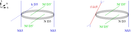
Figure 2: Type IIB brane setup of [4] plus two stacks of $N_{f}$ “flavour” D5-branes before (lhs.) and after the web deformation (rhs.).

This setup preserves $\mathcal{N}=2$ supersymmetry and gives rise to the following $\mathcal{N}=2$ superfields [4]: The NS5-branes divide the D3-brane worldvolume into two intervals along 6. The 3-3 open strings therefore give rise to two $U(N)$ $\mathcal{N}=4$ vector multiplets $(V,\Phi)_{1,2}$ consisting of $\mathcal{N}=2$ vector and chiral multiplets. They also give rise to two complex bifundamental $\mathcal{N}=4$ hypermultiplets $(A,B^{\dagger})_{1,2}$. Furthermore, we note that the (left) NS5-brane splits the $k$ D5-branes into two stacks of $k$ half-D5-branes along the direction 9. This phenomenon is dubbed flavour doubling, see e.g. [22]: Each stack of half D5-branes gives rise to a $U(k)$ global symmetry and provides $2k$ fundamental flavours, i.e. $k$ flavours for each gauge factor. At low energies the 3-5 and 5-3 open string modes therefore generate $k$ fundamental chiral fields $q_{1,2}$, $\tilde{q}_{1,2}$. These fields transform under the $U(k)\times U(k)$ global symmetry as indicated in table 1. The remaining modes coming from strings with both ends on 5-branes are assumed to be decoupled at low energies.

We may now add another class of fundamental fields by introducing $2N_{f}$ “flavour” D$5^{\prime}$-branes along 012789. These branes intersect with the $k$ D5-branes on a three-brane along 0129 and overlap with the D3-branes along 012. This does not break any further supersymmetries, i.e. the total configuration still preserves $\mathcal{N}=2$. At low energies the 3-$5^{\prime}$ and $5^{\prime}$-3 strings give rise to $2N_{f}$ additional fundamental hypermultiplets: $(Q^{r},\tilde{Q}^{r}{}^{\dagger})_{1,2}$ with $r=1,...,N_{f}$. The corresponding $U(N_{f})\times U(N_{f})$ flavour symmetry is non-chiral.

We now perform a web deformation, in which the $k$ D5-branes and the NS5-brane merge into an intermediate $(1,\pm k)5$-brane along $012[3,7]_{\theta_{1}}[4,8]_{\theta_{2}}[5,9]_{\theta_{3}}$, as explained in detail in [4]. This notation means that the $(1,\pm k)5$-brane is aligned along 012 and stretched along directions mixing 345 and 789. Only if the $\theta_{i}$ ($i=1,2,3$) are all the same and satisfy $\tan\theta_{i}=k$ supersymmetry is enhanced from $\mathcal{N}=2$ to $\mathcal{N}=3$ [23, 24].

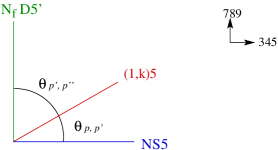
Figure 3: Three types of 5-branes in $\mathbb{E}^{6}$.

The result of this deformation is a triple 5-brane intersection of a $(1,0)5$-brane (NS5-brane), a $(1,k)5$-brane, and two $(0,N_{f})5$-branes ($N_{f}$ D5-branes). These branes overlap over 012, and the remaining directions of the 5-branes form three-planes in the $\mathbb{E}^{6}$ parameterized by $(x^{3},x^{4},x^{5},x^{7},x^{8},x^{9})$. The angle $\theta_{p,q}$ of two of these three-planes is given by [24]

$$\cos\theta_{p,q}=\frac{p\cdot q}{\sqrt{p^{2}{q}^{2}}}\,,$$ (3.1)

where $p\cdot q=p_{i}q_{i}$, and $p,q$ are two of the three $SL(2,\mathbb{Z})$ charge vectors $p=(1,0)$, $p^{\prime}=(1,k)$, $p^{\prime\prime}=(0,N_{f})$. We obtain the angles

$$\tan\theta_{p,p^{\prime}}=k\,, \tan\theta_{p^{\prime},p^{\prime\prime}}=\frac{1}{k}\,, \theta_{p,p^{\prime\prime}}=\frac{\pi}{2}\,,$$ (3.2)

which satisfy $\theta_{p,p^{\prime}}+\theta_{p^{\prime},p^{\prime\prime}}=\theta_{p,p^{\prime\prime}}=\frac{\pi}{2}$. The 5-branes and their intersection angles are shown in figure 3. The rotations in the three three-planes by the same element of $SO(3)_{R}$ correspond to the R-symmetry transformations of the $\mathcal{N}=3$ ultraviolet field theory (2.1)–(2.5) (with $\alpha_{1}=-\alpha_{2}=1$).

We finally note that our setup differs from those considered in [5, 6], which study $\mathcal{N}=2$ supersymmetric Chern-Simons theories with fundamental fields. There the $(1,k)5$-brane is rotated in the 3-7 plane, but not in the 4-8 and 5-9 plane, $\theta_{1}=\theta$, $\theta_{2}=\theta_{3}=0$. Because of this supersymmetry is reduced to $\mathcal{N}=2$ there.

3.1 T-dual setups and lift to M-theory

As in [4] we begin by T-dualizing along the direction 6. The resulting web-deformed type IIA setup then consists of the following branes: The $N$ D3-branes map to $N$ D2-branes along 012, and the NS5-brane turns into a single Kaluza-Klein monopole with world-volume along 012345. The $(1,k)5$ brane is T-dual to an object along $0126[3,7]_{\theta}[4,8]_{\theta}[5,9]_{\theta}$ (with $\tan\theta=k$), which consists of $k$ D6-branes and $1$ KK monopole associated with the 6 direction [4]. In addition we now have $2N_{f}$ D6^′-branes along $0126789$ descending from the flavour D5^′-branes in the type IIB setup.

The type IIA setup may now be lifted to M-theory, where the D2-branes naturally become M2-branes along $012$. The object along $0126[3,7]_{\theta}[4,8]_{\theta}[5,9]_{\theta}$ and the D6^′-branes become KK monopoles with circular direction in 6 and 10 and a linear combination of both [4]. The resulting M-theory configuration will be a stack of $N$ M2-branes located at the origin of a toric hyperkähler manifold [24]. This is an eight-dimensional space ${\cal M}_{8}$ with $sp(2)$ holonomy and preserves $3/16$ of the supersymmetries of the eleven-dimensional supergravity, which is precisely the amount of supersymmetry expected for the dual of theories in 2+1 dimensions with $\mathcal{N}=3$ supersymmetry. Adding a stack of $N$ M2-branes at the origin of ${\cal M}_{8}$ does not break any additional supersymmetry [24].

The metric of ${\cal M}_{8}$ is given by

$$ds^{2}_{{\cal M}_{8}} =U_{ij}d\vec{x}^{i}\cdot d\vec{x}^{j}+U^{ij}(d\varphi_{i}+A_{i})(d\varphi_{j}+A_{j})\,,$$ (3.3)

with the following quantities

$$A_{i}=d\vec{x}^{j}\cdot\vec{\omega}_{ji}=dx^{j}_{a}\omega^{a}_{ji}\,, \partial_{x^{j}_{a}}\omega^{b}_{ki}-\partial_{x^{k}_{b}}\omega^{a}_{ji}=\epsilon^{abc}\partial_{x^{j}_{c}}U_{ki}\,,$$ (3.4)

with $i,j=1,2$. The three-vectors $\vec{x}_{1}$ and $\vec{x}_{2}$ describe positions in two three-planes parameterized by $(x^{7},x^{8},x^{9})$ and $(x^{3},x^{4},x^{5})$, respectively. The two circular directions of the toric geometry are in the directions 6 and 10.

The two-dimensional matrix $U_{ij}$ contains the information of the uplifted five-branes of the IIB setup [24]. Here it is given by

$$U=\mathbf{1}+\begin{pmatrix}h_{1}&0\\ 0&0\end{pmatrix}+\begin{pmatrix}h_{2}&kh_{2}\\ kh_{2}&k^{2}h_{2}\end{pmatrix}+\begin{pmatrix}0&0\\ 0&N^{2}_{f}h_{3}\end{pmatrix}\,,$$ (3.5)

with

$$h_{1}=\frac{1}{2|\vec{x}_{1}|}\,, h_{2}=\frac{1}{2|\vec{x}_{1}+k\vec{x}_{2}|}\,, h_{3}=\frac{1}{|N_{f}\vec{x}_{2}|}\,.$$ (3.6)

The first three terms in (3.5) are as in the ABJM case without flavours [4], while the last term contains the information of the uplifted flavour branes. In the type IIB setup the functions $h_{1,2,3}$ stem from the $(1,0)5$-brane (NS5-brane), the $(1,k)5$-brane, and the (two stacks of) $(0,N_{f})5$-branes (D5-branes), respectively.

An appropriate ansatz for $N$ M2-branes at the origin of ${\cal M}_{8}$ is

$$ds^{2} =H^{-2/3}(-dX_{0}^{2}+dX_{1}^{2}+dX_{2}^{2})+H^{1/3}ds_{{\cal M}_{8}}^{2}\,,$$ (3.7)

$$F =dX_{0}\wedge dX_{1}\wedge dX_{2}\wedge dH^{-1}\,,$$ (3.8)

where the scalar function $H$ only depends on the coordinates of ${\cal M}_{8}$. The supergravity equations of motion then require that $H$ satisfies the Laplace equation on ${\cal M}_{8}$,

$$\partial_{\mu}(\sqrt{g}g^{\mu\nu}\partial_{\nu}H)=0\,,$$ (3.9)

with $g_{\mu\nu}$ given by (3.3).

3.2 Near-horizon geometry

Here we do not attempt to explicitly solve (3.9) but instead explore the hypertoric geometry of the manifold ${\cal M}_{8}$ in more detail. Given the form (3.5) of the matrix $U_{ij}$, we see that the metric (3.3) develops a physical singularity at the point $\vec{x}_{1}=\vec{x}_{2}=0$. In this near-core region the constant piece of the matrix (3.5) is subdominant and can henceforth be dropped. In the following we will carry on to study this region more closely. We begin by presenting the solution to the equations (3.4) by writing an expression for the gauge field one-forms

$$A_{1}=\frac{(x_{12}^{2}dx_{1}^{1}-x_{12}^{1}dx_{1}^{2})+k(x_{12}^{2}dx_{2}^{1}-x_{12}^{1}dx_{2}^{2})}{2|\vec{x}_{12}|(|\vec{x}_{12}|+x_{12}^{3})}+\frac{x_{1}^{2}dx_{1}^{1}-x_{1}^{1}dx_{1}^{2}}{2|\vec{x}_{1}|(|\vec{x}_{1}|+x_{1}^{3})}\,,$$

$$A_{2}=\frac{k(x_{12}^{2}dx_{1}^{1}-x_{12}^{1}dx_{1}^{2})+k^{2}(x_{12}^{2}dx_{2}^{1}-x_{12}^{1}dx_{2}^{2})}{2|\vec{x}_{12}|(|\vec{x}_{12}|+x_{12}^{3})}+\frac{N_{f}(x_{2}^{2}dx_{2}^{1}-x_{2}^{1}dx_{2}^{2})}{|\vec{x}_{2}|(|\vec{x}_{2}|+x_{2}^{3})}\,,$$ (3.10)

where we have introduced the shorthand notation $\vec{x}_{12}=\vec{x}_{1}+k\vec{x}_{2}$. This explicitly determines the metric by inserting (3.10) into (3.3). However, due to the complicated form of (3.10) the complete metric becomes rather difficult to handle and we therefore will not work with it directly.

Instead we want to discuss the isometry group of the geometry (3.3) with solution (3.10). First of all, there are two global $U(1)$ symmetries since (3.3) is invariant under a shift of each of the $\varphi_{i}$ by a constant. We choose to parameterize these $U(1)$s in the following manner

$$U(1)_{\text{gauge}}:\ \left\{\begin{array}[]{ll}\varphi_{1}\longmapsto\varphi_{1}+\lambda_{1}\\ \varphi_{2}\longmapsto\varphi_{2}+\lambda_{1}\end{array}\right.\,, \lambda_{1}\in[0,2\pi)\,,$$ with (3.13)

$$U(1)_{b}:\ \left\{\begin{array}[]{ll}\varphi_{1}\longmapsto\varphi_{1}+\lambda_{2}\\ \varphi_{2}\longmapsto\varphi_{2}-\lambda_{2}\end{array}\right.\,, \lambda_{2}\in[0,2\pi)\,,$$ with (3.16)

where $\lambda_{1}$ and $\lambda_{2}$ are just two constant parameters. The diagonal $U(1)_{\text{gauge}}$ can be promoted to a local symmetry provided that we also transform the gauge potential (3.10). In fact, $U(1)_{\text{gauge}}$ is part of a larger $SU(2)_{\text{gauge}}$ “gauge” symmetry, which acts in the usual way on (3.10)

$$SU(2)_{\text{gauge}}:\,\varphi_{i}\longmapsto\varphi_{i}+\Lambda(\vec{x}_{1},\vec{x}_{2})\,, A_{i}\longmapsto A_{i}-\partial_{i}\Lambda(\vec{x}_{1},\vec{x}_{2})\,.$$ and (3.17)

So far we have only been considering invariances of (3.3) involving $\varphi_{i}$ and $A_{i}$, while there is additionally also an $SO(3)$ symmetry which acts diagonally on $\vec{x}_{1}$ and $\vec{x}_{2}$. As we can see from (3.10), in order to keep the metric (3.3) invariant, such an $SO(3)$ rotation will only close up to a gauge transformation of (3.10). We can, for example, for $\Omega\in SO(3)$ write a transformation which will leave the metric invariant in the following manner

$$SO(3):\,\left\{\begin{array}[]{ccl}(\vec{x}_{1},\vec{x}_{2})&\longmapsto&(\Omega\vec{x}_{1},\Omega\vec{x}_{2})\\ A_{i}&\longmapsto&A_{i}-\partial_{i}h(\Omega,\vec{x}_{1},\vec{x}_{2})\\ \varphi_{i}&\longmapsto&\varphi_{i}+h(\Omega,\vec{x}_{1},\vec{x}_{2})\end{array}\right.\,.$$ (3.21)

Here, according to [25], $h$ is a function of $\Omega$ and $\vec{x}_{1,2}$, which needs to satisfy

$$h(\Omega_{1}\Omega_{2},\vec{x}_{1},\vec{x}_{2})=h(\Omega_{1},\Omega_{2}\vec{x}_{1},\Omega_{2}\vec{x}_{2})+h(\Omega_{2},\vec{x}_{1},\vec{x}_{2})\,, h(\mathbbm{1},\vec{x}_{1},\vec{x}_{2})=0\,.$$ and (3.22)

We can therefore summarize that the complete isometry group of the near-horizon geometry is given by

$$SO(3)\times SU(2)_{\text{gauge}}\times U(1)_{b}\,.$$ (3.23)

This fits nicely with our analysis of the symmetries present in the field theory (see section 2). Indeed, the $SO(3)$ symmetry takes over the role of the $SU(2)$ R-symmetry group, while we can identify $SU(2)_{\text{gauge}}$ with the additional global $SU(2)_{D}$ symmetry present in the dual CFT. As we have already remarked, the global $U(1)_{b}$ is identified with $U(1)_{b}$ of (2.7). We should finally also mention that in the limit $N_{f}=0$ the isometry group (3.23) is in fact enhanced. Most prominently, $SO(3)$, which in (3.21) acts diagonally on $(\vec{x}_{1},\vec{x}_{2})$, is enhanced to $SO(3)\times SO(3)$ acting separately on $\vec{x}_{1}$ and $\vec{x}_{2}$. This in turn means that (3.23) becomes isomorphic to $SU(4)\times U(1)_{b}$, which ties in nicely with the analysis of the symmetries in the dual ABJM-model (see [4]). There it was found, that the three-dimensional Chern-Simons matter theory has an $SU(4)_{R}$ R-symmetry and an additional global baryonic $U(1)$.

4 D6-branes in $AdS_{4}\times{\mathbb{CP}^{3}}$

In the previous section we discussed the fully backreacted solution of the dual gravitational theory. The structure of the corresponding near-horizon geometry is quite involved, which makes a full discussion of the supergravity fluctuations of this background technically difficult. A simpler approach towards a gravity dual of the ABJM theory with flavour is to treat the fundamental fields in the quenched approximation. On the gravity side this corresponds to taking the probe limit [9], in which it is assumed that for a small number of flavours the backreaction of the D6-branes may be ignored. We will therefore embed probe D6-branes into the (type-IIA) near-horizon geometry of the ABJM model, which is $AdS_{4}\times{\mathbb{CP}^{3}}$ [4]. Since flavour branes are spacetime-filling, the D6-branes extend along all the directions of the $AdS_{4}$ space and wrap a Lagrangian-(codimension three)-cycle inside ${\mathbb{CP}^{3}}$. For consistency of the probe approximation, we need to make sure that this cycle is stable and supersymmetric.

The most natural guess for such a Lagrangian subcycle is a real projective space ${\mathbb{RP}^{3}}\subset{\mathbb{CP}^{3}}$. This is due to the well-known mathematical fact that a ${\mathbb{RP}^{3}}$ is among the simplest codimension-three cycles inside ${\mathbb{CP}^{3}}$ [27]. Moreover, it is also known [28] that ${\mathbb{RP}^{3}}$ fulfills certain mathematical stability-criteria under special Hamiltonian deformations. This already points towards the fact that ${\mathbb{RP}^{3}}$ is indeed a stable cycle for the probe D6-brane to wrap.

In the following we will not only show that the configuration of a D6 wrapping a ${\mathbb{RP}^{3}}\subset{\mathbb{CP}^{3}}$ is stable but moreover also supersymmetric. We will proof stability by showing that this cycle gives rise to a generalized calibration 3-form. As a by-product of this computation we will find explicit expressions for the Killing spinors of ${\mathbb{CP}^{3}}$.

4.1 Geometry of ${\mathbb{CP}^{3}}$

4.1.1 Metric and curvature

Let us start by reviewing some basic facts about the $AdS_{4}\times{\mathbb{CP}^{3}}$ supergravity solution. According to [4] the metric, the dilaton and the 2- and 4-form field-strengths are given by

$$ds^{2}=\frac{R^{3}}{k}\left(\frac{1}{4}ds_{Ads_{4}}^{2}+ds_{{\mathbb{CP}^{3}}}^{2}\right), e^{2\phi}=\frac{R^{3}}{k^{3}}\,,$$

$$F^{(2)}_{mn}=kJ_{mn}\,, F^{(4)}_{\mu\nu\rho\tau}=\frac{3R^{3}}{8}\epsilon_{\mu\nu\rho\tau}\,.$$ (4.1)

Here we have used Greek indices $\mu,\nu=1,\ldots,4$ to denote the directions of $AdS_{4}$ and Latin indices $m,n=1,\ldots,6$ for the ${\mathbb{CP}^{3}}$. Moreover, $ds_{{\mathbb{CP}^{3}}}^{2}$ is the standard Fubini-Study metric given by

$$ds_{{\mathbb{CP}^{3}}}^{2}=\frac{d\bar{\zeta}_{\alpha}d\zeta^{\alpha}}{(1+\bar{\zeta}_{\gamma}\zeta^{\gamma})^{2}}+\frac{\zeta^{\alpha}\bar{\zeta}_{\beta}d\bar{\zeta}_{\alpha}d\zeta^{\beta}}{(1+\bar{\zeta}_{\gamma}\zeta^{\gamma})^{4}}\,,$$ (4.2)

with

$$\zeta_{1}=\tan\mu\sin\alpha\sin\frac{\vartheta}{2}e^{\frac{i}{2}(\psi-\varphi+\chi)}\,,$$

$$\zeta_{2}=\tan\mu\cos\alpha e^{\frac{i}{2}\chi}\,,$$

$$\zeta_{3}=\tan\mu\sin\alpha\cos\frac{\vartheta}{2}e^{\frac{i}{2}(\psi+\varphi+\chi)}\,,$$ (4.3)

and $0\leq\mu,\alpha\leq\pi/2$, $0\leq\vartheta\leq\pi$, $0\leq\varphi\leq 2\pi$ [29]. More explicitly, in terms of the left-invariant $SU(2)$ one-forms

$$\sigma_{1}=\cos\psi d\vartheta+\sin\vartheta\sin\psi d\varphi\,, \sigma_{2}=\sin\psi d\vartheta-\sin\vartheta\cos\psi d\varphi\,, \sigma_{3}=d\psi+\cos\vartheta d\varphi\,,$$

the metric $ds_{{\mathbb{CP}^{3}}}^{2}$ can be written as

$$ds_{{\mathbb{CP}^{3}}}^{2}=d\mu^{2}+\sin^{2}\mu \left[d\alpha^{2}+\frac{1}{4}\sin^{2}\alpha(\sigma_{1}^{2}+\sigma_{2}^{2}+\cos^{2}\alpha\sigma_{3}^{2})+\frac{1}{4}\cos^{2}\mu(d\chi+\sin^{2}\alpha\sigma_{3})^{2}\right].$$ (4.4)

The Kähler form $J_{mn}$ is given by

$$J =\frac{1}{2}dA=\frac{1}{4}d\left[\sin^{2}\mu(d\chi+\sin^{2}\alpha\sigma_{3})\right]$$

$$=\sin 2\mu(d\chi+\sin^{2}\alpha(d\psi+\cos\vartheta d\varphi))\wedge d\mu-\frac{1}{4}\sin^{2}\mu\sin^{2}\alpha\sin\vartheta d\varphi\wedge d\vartheta\,.$$ (4.5)

For the choice (4.2) of the metric, ${\mathbb{CP}^{3}}$ is Einstein satisfying the relation

$$R_{mn}=8g_{mn}\,.$$ (4.6)

4.1.2 Lagrangian submanifold

Given the (complex) parameterization (4.3), a ${\mathbb{RP}^{3}}\subset{\mathbb{CP}^{3}}$ is easily found by making sure that $\zeta_{1,2,3}$ all have the same (fixed) complex phase $\omega$. As we can see by a quick inspection, this is achieved by solving

$$\psi-\varphi+\chi=\omega, \chi=\omega, \psi+\varphi+\chi=\omega\,.$$ (4.7)

For the simplest choice $\omega=0$ the solution $\psi=\varphi=\chi=0$ yields a manifestly real parameterization of ${\mathbb{RP}^{3}}=S^{3}/\mathbb{Z}_{2}$ with the standard metric

$$ds_{{\mathbb{RP}^{3}}}^{2}=d\mu^{2}+\sin^{2}\mu d\alpha^{2}+\frac{1}{4}\sin^{2}\alpha\sin^{2}\mu d\vartheta^{2}\,.$$ (4.8)

The isometry group of ${\mathbb{RP}^{3}}$ is $\mathbb{Z}_{2}\ltimes(SO(3)\times SO(3))$, where $\ltimes$ denotes a semi-direct product. This means the isometry group consists of two $SO(3)$ groups and a discrete symmetry exchanging the two $SO(3)$ groups, see e.g. [30]. The occurrence of two $SO(3)$’s reflect the $SU(2)$ R-symmetry and the global $SU(2)_{D}$ symmetry of the field theory. In the following we will show that a D6-brane wrapped around this submanifold is indeed a stable and supersymmetric configuration.

4.2 Killing spinors of ${\mathbb{CP}^{3}}$

For the construction of a bispinor 3-form in the next subsection, we will need the Killing spinors of ${\mathbb{CP}^{3}}$. It is a well-known fact [31] that there are six Killing spinors on ${\mathbb{CP}^{3}}$. They can be found as solutions of the following two equations, which stem from the supervariations of the fermionic degrees of freedom in supergravity

$$D_{m}\epsilon-\frac{1}{32}\left(\Gamma_{m}Q+16\tilde{\Gamma}_{m}\Gamma_{0}\right)\epsilon-\frac{9}{16}\Gamma_{m}\epsilon=0\,,$$ (4.9)

$$\frac{3}{8\sqrt{2}}Q\Gamma_{0}\epsilon+\frac{3}{4\sqrt{2}}\Gamma_{0}\epsilon=0\,.$$ (4.10)

Here we have introduced the quantities

$$Q=J^{mn}\Gamma_{mn}\Gamma_{0}\,, \tilde{\Gamma}_{m}={J_{m}}^{n}\Gamma_{n}\,.$$ and (4.11)

Moreover, $\Gamma_{m}$ are the six-dimensional Dirac matrices. Relation (4.10) is an eigenspinor relation for the operator $Q$, and it was shown in [31] that $Q$ has the following eigenvalues

$$\{-2,-2,-2,-2,-2,-2,6,6\}\,.$$ (4.12)

Since we know that the background $AdS_{4}\times{\mathbb{CP}^{3}}$ preserves $\mathcal{N}=6$ supersymmetry, we conclude that we need to look for eigenspinors to the eigenvalue $-2$ because the latter has a 6-fold degeneracy. The most general spinor compatible with this eigenvalue is given by

$$\epsilon=\left(\begin{array}[]{c}f_{1}+f_{2}+f_{6}\\ -f_{6}\\ -f_{3}+f_{4}+f_{5}\\ f_{5}\\ f_{4}\\ f_{3}\\ f_{2}\\ f_{1}\end{array}\right),$$ (4.21)

where $f_{i=1,\ldots,6}$ are six arbitrary functions of the coordinates $(\mu,\alpha,\vartheta,\varphi,\psi,\chi)$. The exact functional dependence can be fixed by inserting this ansatz into the remaining killing spinor equation (4.9). This yields a system of coupled first order partial differential equations, which can be solved analytically. Since the computations are rather tedious, we will not relate all the details here, but content ourselves by giving the explicit solution in appendix B.

4.3 Embedding of D6-branes

The Killing spinors of ${\mathbb{CP}^{3}}$ can now be used to compute the bispinor 3-form

$$\Omega_{mnp}=\bar{\epsilon}\Gamma_{mnp}\epsilon\,.$$ (4.22)

Since the full $\Omega$ is a rather lengthy expression, we refrain from writing it down completely, but only display the relevant component. Following our logic in section 4.1.2 concerning the Lagrangian submanifold, the latter is parameterized by $(\mu,\alpha,\vartheta)$, while $(\psi,\varphi,\chi)$ are set to constant values. Therefore, the relevant component of $\Omega$ is $\Omega_{\mu\alpha\vartheta}$ given by

$$\Omega_{\mu\alpha\vartheta}= \frac{1}{2}e^{-\frac{i}{2}(2\varphi+\chi+2\psi)}\left(e^{i(\varphi+\chi+2\psi)}\lambda_{1}^{2}+e^{i\varphi}\lambda_{2}^{2}+e^{i\psi}\left(\lambda_{4}^{2}+e^{2i\varphi}\lambda_{6}^{2}+e^{i\chi}\left(e^{2i\varphi}\lambda_{3}^{2}+\lambda_{5}^{2}\right)\right)\right)$$

$$\times\sin\alpha\sin^{2}\mu\,.$$ (4.23)

Notice that this is a complex expression, which we can separate into real and imaginary part

$$\text{Re}(\Omega_{\mu\alpha\vartheta})=\frac{1}{2}\sin\alpha\sin^{2}\mu$$ (4.24)

$$\hskip 8.5359pt\times\left(\left(\lambda_{5}^{2}+\lambda_{6}^{2}\right)\cos\left(\phi-\frac{\chi}{2}\right)+\left(\lambda_{3}^{2}+\lambda_{4}^{2}\right)\cos\left(\phi+\frac{\chi}{2}\right)+\left(\lambda_{1}^{2}+\lambda_{2}^{2}\right)\cos\left(\frac{\chi}{2}+\psi\right)\right),$$

$$\text{Im}(\Omega_{\mu\alpha\vartheta})=-\frac{1}{2}\sin\alpha\sin^{2}\mu$$ (4.25)

$$\hskip 8.5359pt\times\left((\lambda_{5}^{2}-\lambda_{6}^{2})\sin\left(\phi-\frac{\chi}{2}\right)+\left(\lambda_{4}^{2}-\lambda_{3}^{2}\right)\sin\left(\phi+\frac{\chi}{2}\right)+\left(\lambda_{2}^{2}-\lambda_{1}^{2}\right)\sin\left(\frac{\chi}{2}+\psi\right)\right).$$

Following [32], in order to be a real calibration form the restriction of $\Omega$ to the Lagrangian submanifold needs to satisfy

$$\text{Im}(\Omega)_{\big{|}\psi=\varphi=\chi=0}=0\,, \text{Re}(\Omega)_{\big{|}\psi=\varphi=\chi=0}\simeq\text{Vol}_{{\mathbb{RP}^{3}}}\,,$$ and (4.26)

where $\text{Vol}_{{\mathbb{RP}^{3}}}$ is the volume form of the submanifold. Inserting (4.24) and (4.25) into (4.26) we indeed find

$$\text{Im}(\Omega)_{\big{|}\psi=\varphi=\chi=0}=0\,,$$ (4.27)

$$\text{Re}(\Omega)_{\big{|}\psi=\varphi=\chi=0}=\frac{1}{2}(\lambda_{1}^{2}+\lambda_{2}^{2}+\lambda_{3}^{2}+\lambda_{4}^{2}+\lambda_{5}^{2}+\lambda_{6}^{2})\sin\alpha\sin^{2}\mu\,.$$ (4.28)

Comparing to (4.8) we see that this is indeed proportional to the volume form of ${\mathbb{RP}^{3}}$ showing that $\Omega$ is indeed a calibration form. The chosen embedding of the D6-branes is thus stable and supersymmetric. Naively, we expect that the D6-brane embedding breaks half of the supersymmetries of the $AdS_{4}\times{\mathbb{CP}^{3}}$ background, which ties in with the $\mathcal{N}=3$ supersymmetry of the field theory. Clearly, to show this precisely would require a careful analysis of the $\kappa$-symmetry.

5 Conclusions and open questions

In this note we discussed an $\mathcal{N}=3$ version of the ABJM model with $2N_{f}$ fields in the fundamental representation of the $U(N)_{k}\times U(N)_{-k}$ gauge group. The theory has a dual description in terms of $N$ M2-branes at a hypertoric geometry ${\cal M}_{8}$, given by the metric (3.3) with (3.5) and (3.10). We argued that the isometry of ${\cal M}_{8}$ is $SU(2)\times SU(2)\times U(1)$, which matches to the $SU(2)$ R-symmetry of $\mathcal{N}=3$ supersymmetry, a global $SU(2)_{D}$ symmetry and a $U(1)_{b}$ “baryonic” symmetry in the dual field theory. Of course, a complete construction of the near-horizon geometry would require to also determine the harmonic function $H$ of the geometry by solving the Laplace equation (3.9), possibly along the lines of [34].

Another approach outlined in this paper is to consider the “flavour” D6-branes in the probe approximation, which corresponds to quenched flavours in the field theory. This requires the embedding of the D6-branes into the $AdS_{4}\times{\mathbb{CP}^{3}}$ near-horizon geometry of the ABJM model. We showed that ${\mathbb{RP}^{3}}$ is a special Lagrangian three-cycle in ${\mathbb{CP}^{3}}$ and that D6-branes wrapping $AdS_{4}\times{\mathbb{RP}^{3}}$ are stable and supersymmetric. Since the isometries of ${\mathbb{RP}^{3}}$ match again the global symmetries of the field theory, we expect that fluctuations of the D6-branes are dual to bound state operators of (massless) fundamentals. It would be interesting to verify this by an explicit calculation. This could possibly be done (numerically) using the Dirac-Born-Infeld action evaluated on the world-volume of the D6-branes. We leave this for future work.

Appendix A Symmetries of the action

In this section we will explore the symmetry content of the action (2.1)–(2.3) for the particular values $\alpha_{1}=-\alpha_{2}=1$. In the way (2.1)–(2.3) is written only $\mathcal{N}=2$ supersymmetry is manifest. In order to exhibit a possible enhancement of the latter we need to get rid of the auxiliary fields as they are intimately tied to the $\mathcal{N}=2$ superspace formulation. We therefore need to work out the action in component formulation. To this end, we recall the Grassmann expansion of all superfields involved. The chiral superfields are of the form

$$A_{i}=a_{i}+\sqrt{2}\theta\psi^{(A)}_{i}+\theta^{2}F^{(A)}_{i}\,, B_{i}=b_{i}+\sqrt{2}\theta\psi^{(B)}_{i}+\theta^{2}F^{(B)}_{i}\,,$$ (A.1)

$$Q_{i}^{r}=q_{i}^{r}+\sqrt{2}\theta\zeta^{r}_{i}+\theta^{2}G^{r}_{i}\,, \tilde{Q}^{r}_{i}=\tilde{q}_{i}^{r}+\sqrt{2}\theta\tilde{\zeta}^{r}_{i}+\theta^{2}\tilde{G}^{r}_{i}\,,$$ (A.2)

while the vector superfields have the expansion

$$V_{i}=2i\theta\bar{\theta}\sigma_{i}+2\theta\gamma^{\mu}\bar{\theta}A_{\mu,i}+\sqrt{2}i\theta^{2}\bar{\theta}\bar{\chi}_{i}-\sqrt{2}i\bar{\theta}^{2}\theta\chi_{i}+\theta^{2}\bar{\theta}^{2}D_{i}\quad(i=1,2)\,.$$ (A.3)

Although we have also explicitly written down fermionic components in the Grassmann expansion, we will in the following only focus on the scalar fields, namely $(a_{i},b_{i},q_{1,2}^{r},\tilde{q}_{1,2}^{r})$. It is then straight-forward to eliminate the auxiliary fields $(F^{(A,B)}_{i},G^{r}_{1,2},\tilde{G}^{r}_{1,2},\sigma_{i},D_{i})$ from the action (2.1)–(2.3), after which the pure scalar part becomes

$$S=\frac{4\pi^{2}}{3k^{2}}\big{[} q_{a}^{1}\bar{q}^{a}_{1}q_{b}^{1}\bar{q}^{b}_{1}q_{c}^{1}\bar{q}^{c}_{1}+q_{a}^{2}\bar{q}^{a}_{2}q_{b}^{2}\bar{q}^{b}_{2}q_{c}^{2}\bar{q}^{c}_{2}-4q_{a}^{1}\bar{q}^{b}_{1}q_{c}^{1}\bar{q}^{a}_{1}q_{b}^{1}\bar{q}^{c}_{1}-4q_{a}^{2}\bar{q}^{b}_{2}q_{c}^{2}\bar{q}^{a}_{2}q_{b}^{2}\bar{q}^{c}_{2}+$$

$$+ a_{a}^{i}\bar{a}^{a}_{i}a_{b}^{j}\bar{a}^{b}_{j}a_{c}^{k}\bar{a}^{c}_{k}+\bar{a}^{a}_{i}a_{a}^{i}\bar{a}^{b}_{j}a_{b}^{j}\bar{a}^{c}_{k}a_{c}^{k}+4a_{a}^{i}\bar{a}^{b}_{j}a_{c}^{k}\bar{a}^{a}_{i}a_{b}^{j}\bar{a}^{c}_{k}-6a_{a}^{i}\bar{a}^{b}_{j}a_{b}^{j}\bar{a}^{a}_{i}a_{c}^{k}\bar{a}^{c}_{k}$$

$$+ 3a_{a}^{i}\bar{a}^{a}_{i}a_{b}^{j}\bar{a}^{b}_{j}q_{c}^{1}\bar{q}^{c}_{1}+3\bar{a}^{a}_{i}a_{a}^{i}\bar{a}^{b}_{j}a_{b}^{j}\bar{q}^{c}_{2}q_{c}^{2}-6a_{a}^{i}\bar{a}^{b}_{j}a_{b}^{j}\bar{a}^{a}_{i}q_{c}^{1}\bar{q}^{c}_{1}-6\bar{a}^{a}_{i}a_{b}^{j}\bar{a}^{b}_{j}a_{a}^{i}\bar{q}^{c}_{2}q_{c}^{2}$$

$$+ 9a_{a}^{i}\bar{a}^{a}_{i}q_{b}^{1}\bar{q}^{b}_{1}q_{c}^{1}\bar{q}^{c}_{1}+9\bar{a}^{a}_{i}a_{a}^{i}\bar{q}^{b}_{2}q_{b}^{2}\bar{q}^{c}_{2}q_{c}^{2}-6a_{a}^{i}\bar{a}^{a}_{i}q_{b}^{1}\bar{q}^{c}_{1}q_{c}^{1}\bar{q}^{b}_{1}-6\bar{a}^{a}_{i}a_{a}^{i}\bar{q}^{b}_{2}q_{c}^{2}\bar{q}^{c}_{2}q_{b}^{2}$$

$$- 6a_{a}^{i}\bar{a}^{b}_{i}q_{b}^{1}\bar{q}^{a}_{1}q_{c}^{1}\bar{q}^{c}_{1}-6\bar{a}^{a}_{i}a_{b}^{i}\bar{q}^{b}_{2}q_{a}^{2}\bar{q}^{c}_{2}q_{c}^{2}+6a_{a}^{i}\bar{a}^{b}_{i}q_{b}^{1}\bar{q}^{c}_{1}q_{c}^{1}\bar{q}^{a}_{1}+6\bar{a}^{a}_{i}a_{b}^{i}\bar{q}^{b}_{2}q_{c}^{2}\bar{q}^{c}_{2}q_{a}^{2}$$

$$- 6a_{a}^{i}\bar{a}^{b}_{i}q_{c}^{1}\bar{q}^{a}_{1}q_{b}^{1}\bar{q}^{c}_{1}-6\bar{a}^{a}_{i}a_{b}^{i}\bar{q}^{c}_{2}q_{a}^{2}\bar{q}^{b}_{2}q_{c}^{2}-6a_{a}^{i}\bar{a}^{b}_{i}q_{c}^{1}\bar{q}^{c}_{1}q_{b}^{1}\bar{q}^{a}_{1}-6\bar{a}^{b}_{i}a_{a}^{i}\bar{q}^{c}_{2}q_{c}^{2}\bar{q}^{a}_{2}q_{b}^{2}-$$

$$- 6\bar{a}^{a}_{i}q_{b}^{1}\bar{q}^{b}_{1}a_{a}^{i}\bar{q}^{c}_{2}q_{c}^{2}+12\bar{a}^{a}_{i}q_{b}^{1}\bar{q}^{c}_{1}a_{a}^{i}\bar{q}^{b}_{2}q_{c}^{2}+12\epsilon_{ij}\epsilon^{kl}a_{c}^{i}\bar{a}^{b}_{k}a_{a}^{j}\bar{a}^{c}_{l}q_{b}^{1}\bar{q}^{a}_{1}$$

$$+ 12\epsilon^{ij}\epsilon_{kl}\bar{a}^{c}_{i}a_{b}^{k}\bar{a}^{a}_{j}a_{c}^{l}\bar{q}^{b}_{2}q_{a}^{2}\big{]}\,,$$ (A.4)

where flavour indices are suppressed. Here we have arranged all fields in the following doublet form

$$a_{a}^{i}=\left(\begin{array}[]{c}a_{i}\\ \bar{b}_{i}\end{array}\right)\,, q_{a}^{1}=\left(\begin{array}[]{c}q_{1}\\ \bar{\tilde{q}}_{1}\end{array}\right)\,, q_{a}^{2}=\left(\begin{array}[]{c}\tilde{q}_{2}\\ \bar{q}_{2}\end{array}\right)\,,$$ and and (A.11)

which exhibits invariance of (A.4) under two types of $SU(2)$ symmetries. First of all, we find a $SU(2)_{R}$ R-symmetry, which acts on the indices $a,b=1,2$. This symmetry acts on the bifundamental fields $a_{a}^{i}$ as well as on the flavours $q_{a}^{1,2}$. Apart from this, there is yet another $SU(2)$, which acts on the index $i,j=1,2$. We call this symmetry $SU(2)_{D}$ as it can be understood to be the diagonal of the $SU(2)_{A}\times SU(2)_{B}$ global symmetry, which has already been described in [4]. It is, however, important to notice that in contrast to the pure ABJM-case this $SU(2)_{D}$ commutes with the R-symmetry group $SU(2)_{R}$ and therefore does not lead to an additional enhancement of the $SU(2)_{R}$ R-symmetry group.

As a side remark, we note that the first four lines of (A.4) are invariant under a larger $SU(2)_{a}\times SU(2)_{q}$ symmetry rotating separately $a_{a}^{i}$ and $q^{1,2}_{a}$. However, the last four lines of (A.4) contain contractions between the $a_{a}^{i}$ and $q^{i}_{a}$ fields breaking $SU(2)_{a}\times SU(2)_{q}$ down to $SU(2)_{R}$.

Appendix B Killing spinors of ${\mathbb{CP}^{3}}$

According to the reasoning of section 4.2, we expect to find a six-dimensional solution space to the Killing spinor equation, which is parameterized by the integration constants $\lambda_{1},\ldots,\lambda_{6}$. With these parameters, we can state the final result for the general Killing spinor defined in (4.21):

$$f_{1} =\frac{1}{2}e^{-\frac{i}{4}(2\varphi+\chi+2\psi)}\bigg{[}e^{\frac{i}{2}(\varphi+\chi+2\psi)}{\lambda_{5}}(\cos\alpha+i\cos\mu\sin\alpha)-e^{\frac{i}{2}\varphi}{\lambda_{6}}\sin\alpha\sin\mu$$

$$\hskip 14.22636pt+e^{\frac{i}{2}\psi}\bigg{(}e^{\frac{i}{2}\chi}\bigg{(}\cos(\vartheta/2)\left(\left(e^{i\varphi}{\lambda_{1}}-i{\lambda_{3}}\cos\alpha\right)\cos\mu+{\lambda_{3}}\sin\alpha\right)$$ (B.1)

$$\hskip 14.22636pt+\bigg{(}e^{i\varphi}{\lambda_{1}}(\sin\alpha-i\cos\alpha\cos\mu)-{\lambda_{3}}\cos\mu\bigg{)}\sin(\vartheta/2)\bigg{)}$$

$$\hskip 14.22636pt+\sin\mu\bigg{(}\left(i{\lambda_{2}}+e^{i\varphi}{\lambda_{4}}\cos\alpha\right)\cos(\vartheta/2)+\sin(\vartheta/2)({\lambda_{2}}\cos\alpha+{\lambda_{4}}(\sin\varphi-i\cos\varphi))\bigg{)}\bigg{)}\bigg{]},$$

$$f_{2} =\frac{1}{2}e^{-\frac{i}{4}(2\varphi+\chi+2\psi)}\bigg{[}-e^{\frac{i}{2}(\varphi+\chi+2\psi)}{\lambda_{5}}(\cos\alpha+i\cos\mu\sin\alpha)-e^{\frac{i}{2}\varphi}{\lambda_{6}}\sin\alpha\sin\mu$$

$$\hskip 14.22636pt+e^{\frac{i}{2}\psi}\bigg{(}e^{\frac{i}{2}\chi}\bigg{(}\cos(\vartheta/2)\left(\left(e^{i\varphi}{\lambda_{1}}+i{\lambda_{3}}\cos\alpha\right)\cos\mu-{\lambda_{3}}\sin\alpha\right)$$

$$\hskip 14.22636pt-\left({\lambda_{3}}\cos\mu+e^{i\varphi}{\lambda_{1}}(\sin\alpha-i\cos\alpha\cos\mu)\right)\sin(\vartheta/2)\bigg{)}$$

$$\hskip 14.22636pt+\left(\left(e^{i\varphi}{\lambda_{4}}\cos\alpha-i{\lambda_{2}}\right)\cos(\vartheta/2)+\left(ie^{i\varphi}{\lambda_{4}}+{\lambda_{2}}\cos\alpha\right)\sin(\vartheta/2)\right)\sin\mu\bigg{)}\bigg{]},$$ (B.2)

$$f_{3} =\frac{1}{2}e^{-\frac{i}{2}(\varphi+\psi)}\bigg{[}e^{\frac{i}{4}(2\varphi-\chi)}{\lambda_{6}}(\cos\alpha+\cos\mu\sin\alpha)-e^{\frac{i}{4}(2\varphi+\chi+4\psi)}{\lambda_{5}}\sin\alpha\sin\mu$$

$$\hskip 14.22636pt+e^{-\frac{i}{4}(\chi-2\psi)}\bigg{(}\sin(\vartheta/2)\bigg{(}\left(-e^{i\varphi}{\lambda_{4}}-i{\lambda_{2}}\cos\alpha\right)\cos\mu+{\lambda_{2}}\sin\alpha$$

$$\hskip 14.22636pt+e^{\frac{i}{2}\chi}\left(e^{i\varphi}{\lambda_{1}}\cos\alpha-i{\lambda_{3}}\right)\sin\mu\bigg{)}+\cos(\vartheta/2)\big{(}e^{i\varphi}{\lambda_{4}}\sin\alpha$$

$$\hskip 14.22636pt+e^{\frac{i}{2}\chi}\left(ie^{i\varphi}{\lambda_{1}}+{\lambda_{3}}\cos\alpha\right)\sin\mu+\cos\mu({\lambda_{2}}-ie^{i\varphi}{\lambda_{4}}\cos\alpha)\big{)}\bigg{)}\bigg{]},$$ (B.3)

$$f_{4} =\frac{1}{2}e^{-\frac{i}{2}(\varphi+\psi)}\bigg{[}e^{\frac{i}{4}(2\varphi-\chi)}{\lambda_{6}}(\cos\alpha+i\cos\mu\sin\alpha)+e^{\frac{i}{4}(2\varphi+\chi+4\psi)}{\lambda_{5}}\sin\alpha\sin\mu$$

$$\hskip 14.22636pt+e^{-\frac{i}{4}(\chi-2\psi)}\bigg{(}\sin(\vartheta/2)\bigg{(}\left(e^{i\varphi}{\lambda_{4}}-i{\lambda_{2}}\cos\alpha\right)\cos\mu+{\lambda_{2}}\sin\alpha$$

$$\hskip 14.22636pt-e^{\frac{i}{2}\chi}\left(i{\lambda_{3}}+e^{i\varphi}{\lambda_{1}}\cos\alpha\right)\sin\mu\bigg{)}+\cos(\vartheta/2)\bigg{(}\left(-{\lambda_{2}}-ie^{i\varphi}{\lambda_{4}}\cos\alpha\right)\cos\mu$$

$$\hskip 14.22636pt+e^{i\varphi}{\lambda_{4}}\sin\alpha-e^{\frac{i}{2}}\sin\mu({\lambda_{3}}\cos\alpha-ie^{i\varphi}{\lambda_{1}})\bigg{)}\bigg{)}\bigg{]},$$ (B.4)

$$f_{5} =\frac{1}{2}e^{-\frac{i}{2}(\varphi+\psi)}\bigg{[}-e^{\frac{i}{4}(2\varphi-\chi)}{\lambda_{6}}(\cos\alpha-i\cos\mu\sin\alpha)-e^{\frac{i}{4}(2\varphi+\chi+4\psi)}{\lambda_{5}}\sin\alpha\sin\mu$$

$$\hskip 14.22636pt+e^{-\frac{i}{4}(\chi-2\psi)}\bigg{(}\sin(\vartheta/2)\bigg{(}\left(-e^{i\varphi}{\lambda_{4}}-i{\lambda_{2}}\cos\alpha\right)\cos\mu-{\lambda_{2}}\sin\alpha$$

$$\hskip 14.22636pt+e^{\frac{i}{2}\chi}\left(e^{i\varphi}{\lambda_{1}}\cos\alpha-i{\lambda_{3}}\right)\sin\mu\bigg{)}+\cos(\vartheta/2)\bigg{(}-e^{i\varphi}{\lambda_{4}}\sin\alpha$$

$$\hskip 14.22636pt+e^{\frac{i}{2}\chi}\left(ie^{i\varphi}{\lambda_{1}}+{\lambda_{3}}\cos\alpha\right)\sin\mu+\cos\mu({\lambda_{2}}-ie^{i\varphi}{\lambda_{4}}\cos\alpha)\bigg{)}\bigg{)}\bigg{]},$$ (B.5)

$$f_{6} =-\frac{1}{2}e^{-\frac{i}{4}(2\varphi+\chi+2\psi)}\bigg{[}-e^{\frac{i}{2}(\varphi+\chi+2\psi)}{\lambda_{5}}(\cos\alpha-i\cos\mu\sin\alpha)-e^{\frac{i}{2}\varphi}{\lambda_{6}}\sin\alpha\sin\mu$$

$$\hskip 14.22636pt+e^{\frac{i}{2}\psi}\bigg{(}e^{\frac{i}{2}\chi}\big{(}\cos(\vartheta/2)\left(\left(e^{i\varphi}{\lambda_{1}}-i{\lambda_{3}}\cos\alpha\right)\cos\mu-{\lambda_{3}}\sin\alpha\right)$$ (B.6)

$$\hskip 14.22636pt+\left({\lambda_{3}}\cos\mu+e^{i\varphi}{\lambda_{1}}(i\cos\alpha\cos\mu+\sin\alpha)\right)\sin(\vartheta/2)\big{)}$$

$$\hskip 14.22636pt+\sin\mu\left(\left(i{\lambda_{2}}+e^{i\varphi}{\lambda_{4}}\cos\alpha\right)\cos(\vartheta/2)+\sin(\vartheta/2)({\lambda_{2}}\cos\alpha-ie^{i\varphi}{\lambda_{4}})\right)\bigg{)}\bigg{]}.$$

References

• [1] J. Bagger and N. Lambert, Modeling multiple M2’s, Phys. Rev.  D 75, 045020 (2007) [arXiv:hep-th/0611108]; J. Bagger and N. Lambert, Gauge Symmetry and Supersymmetry of Multiple M2-Branes, Phys. Rev.  D 77, 065008 (2008) [arXiv:0711.0955 [hep-th]]; J. Bagger and N. Lambert, Comments On Multiple M2-branes, JHEP 0802, 105 (2008) [arXiv:0712.3738 [hep-th]];
• [2] A. Gustavsson, Algebraic structures on parallel M2-branes, Nucl. Phys.  B 811, 66 (2009) [arXiv:0709.1260 [hep-th]]. A. Gustavsson, Selfdual strings and loop space Nahm equations, JHEP 0804, 083 (2008) [arXiv:0802.3456 [hep-th]];
• [3] M. Van Raamsdonk, Comments on the Bagger-Lambert theory and multiple M2-branes, JHEP 0805, 105 (2008) [arXiv:0803.3803 [hep-th]].
• [4] O. Aharony, O. Bergman, D. L. Jafferis and J. Maldacena, N=6 superconformal Chern-Simons-matter theories, M2-branes and their gravity duals, JHEP 0810, 091 (2008) [arXiv:0806.1218 [hep-th]].
• [5] A. Giveon and D. Kutasov, Seiberg Duality in Chern-Simons Theory, Nucl. Phys.  B 812, 1 (2009) [arXiv:0808.0360 [hep-th]].
• [6] V. Niarchos, Seiberg Duality in Chern-Simons Theories with Fundamental and Adjoint Matter, JHEP 0811, 001 (2008) [arXiv:0808.2771 [hep-th]].
• [7] V. Niarchos, R-charges, Chiral Rings and RG Flows in Supersymmetric Chern-Simons-Matter Theories, arXiv:0903.0435 [hep-th].
• [8] J. Erdmenger, N. Evans, I. Kirsch and E. Threlfall, Mesons in Gauge/Gravity Duals - A Review, Eur. Phys. J.  A 35, 81 (2008) [arXiv:0711.4467 [hep-th]].
• [9] A. Karch and E. Katz, Adding flavor to AdS/CFT, JHEP 0206, 043 (2002) [arXiv:hep-th/0205236].
• [10] M. Kruczenski, D. Mateos, R. C. Myers and D. J. Winters, Meson spectroscopy in AdS/CFT with flavour, JHEP 0307, 049 (2003) [arXiv:hep-th/0304032].
• [11] J. Babington, J. Erdmenger, N. J. Evans, Z. Guralnik and I. Kirsch, Chiral symmetry breaking and pions in non-supersymmetric gauge / gravity duals, Phys. Rev. D 69, 066007 (2004) [arXiv:hep-th/0306018].
• [12] D. Gaiotto and D. L. Jafferis, Notes on adding D6 branes wrapping RP3 in AdS4 x CP3, arXiv:0903.2175 [hep-th].
• [13] Y. Hikida, W. Li and T. Takayanagi, ABJM with Flavors and FQHE, arXiv:0903.2194 [hep-th].
• [14] I. R. Klebanov and E. Witten, Superconformal field theory on threebranes at a Calabi-Yau singularity, Nucl. Phys.  B 536, 199 (1998) [arXiv:hep-th/9807080].
• [15] S. Kuperstein, Meson spectroscopy from holomorphic probes on the warped deformed conifold, JHEP 0503, 014 (2005) [arXiv:hep-th/0411097].
• [16] P. Ouyang, Holomorphic D7-branes and flavored N = 1 gauge theories, Nucl. Phys.  B 699, 207 (2004) [arXiv:hep-th/0311084]; T. S. Levi and P. Ouyang, Mesons and Flavor on the Conifold, Phys. Rev. D 76, 105022 (2007) [arXiv:hep-th/0506021].
• [17] M. Benna, I. Klebanov, T. Klose and M. Smedback, Superconformal Chern-Simons Theories and $AdS_{4}/CFT_{3}$ Correspondence, JHEP 0809, 072 (2008) [arXiv:0806.1519 [hep-th]].
• [18] D. L. Jafferis and X. Yin, Chern-Simons-Matter Theory and Mirror Symmetry, arXiv:0810.1243 [hep-th].
• [19] D. Gaiotto and X. Yin, Notes on superconformal Chern-Simons-matter theories, JHEP 0708, 056 (2007) [arXiv:0704.3740 [hep-th]].
• [20] A. N. Kapustin and P. I. Pronin, Nonrenormalization theorem for gauge coupling in (2+1)-dimensions, Mod. Phys. Lett.  A 9, 1925 (1994) [arXiv:hep-th/9401053].
• [21] L. V. Avdeev, D. I. Kazakov and I. N. Kondrashuk, Renormalizations in supersymmetric and nonsupersymmetric nonAbelian Chern-Simons field theories with matter, Nucl. Phys.  B 391, 333 (1993); L. V. Avdeev, G. V. Grigorev and D. I. Kazakov, Renormalizations in Abelian Chern-Simons field theories with matter, Nucl. Phys.  B 382, 561 (1992).
• [22] J. Park, R. Rabadan and A. M. Uranga, N = 1 type IIA brane configurations, chirality and T-duality, Nucl. Phys.  B 570, 3 (2000) [arXiv:hep-th/9907074].
• [23] T. Kitao, K. Ohta and N. Ohta, Three-dimensional gauge dynamics from brane configurations with (p,q)-fivebrane, Nucl. Phys.  B 539, 79 (1999) [arXiv:hep-th/9808111].
• [24] J. P. Gauntlett, G. W. Gibbons, G. Papadopoulos and P. K. Townsend, Hyper-Kaehler manifolds and multiply intersecting branes, Nucl. Phys.  B 500, 133 (1997) [arXiv:hep-th/9702202].
• [25] I. I. Cotaescu and M. Visinescu, The induced representation of the isometry group of the Euclidean Taub-NUT space and new spherical harmonics, Mod. Phys. Lett.  A 19 (2004) 1397 [arXiv:hep-th/0312129].
• [26] D. Arean, D. E. Crooks and A. V. Ramallo, Supersymmetric probes on the conifold, JHEP 0411, 035 (2004) [arXiv:hep-th/0408210].
• [27] R. Chiang, Nonstandard Lagrangian Submanifolds in $\mathbb{C}\mathbb{P}^{n}$, arXiv:math/0303262 [math.SG]
• [28] Yong-Geun Oh, Second variation and stabilities of minimal lagrangian submanifolds in Kähler manifolds, Invent. math. 101, 501 (1990); Yong-Geun Oh, Volume minimization of Lagrangian submanifolds under Hamiltonian deformations, Math. Z. 212, 175 (1993).
• [29] C. N. Pope and N. P. Warner, An $SU(4)$ invariant compactification of the $d=11$ Supergravity on a strechted seven-sphere, Phys. Lett. B 150, 352 (1985).
• [30] B. McInnes, De Sitter and Schwarzschild-de Sitter according to Schwarzschild and de Sitter, JHEP 0309, 009 (2003) [arXiv:hep-th/0308022].
• [31] B. E. W. Nilsson and C. N. Pope, Hopf Fibration Of Eleven-Dimensional Supergravity, Class. Quant. Grav.  1, 499 (1984).
• [32] J.F.G. Cascales and A.M. Uranga, Branes on Generalized Calibrated Submanifolds, JHEP 0411, 083 (2004) [arXiv:hep-th/0407132]; J. Dadok and F. R. Harvey, Calibrations and spinors, Acta. Math. 170, 83 (1993); J. Gutowski, G. Papadopoulos and P. K. Townsend, Supersymmetry and generalized calibrations, Phys. Rev.  D 60, 106006 (1999) [arXiv:hep-th/9905156].
• [33] P. Koerber and L. Martucci, JHEP 0801, 047 (2008) [arXiv:0710.5530 [hep-th]]; P. Koerber, Stable D-branes, calibrations and generalized Calabi-Yau geometry, JHEP 0508, 099 (2005) [arXiv:hep-th/0506154]; L. Martucci and P. Smyth, Supersymmetric D-branes and calibrations on general N = 1 backgrounds, JHEP 0511, 048 (2005) [arXiv:hep-th/0507099].
• [34] A. Hashimoto and P. Ouyang, Supergravity dual of Chern-Simons Yang-Mills theory with N=6,8 superconformal IR fixed JHEP 0810, 057 (2008) [arXiv:0807.1500 [hep-th]].