Stationary light in cold atomic gases

Abstract

We discuss stationary light created by a pair of counter-propagating control fields in $\Lambda$-type atomic gases with electromagnetically induced transparency for the case of negligible Doppler broadening. In this case the secular approximation used in the discussion of stationary light in hot vapors is no longer valid. We discuss the quality of the effective light-trapping system and show that in contrast to previous claims it is finite even for vanishing ground-state dephasing. The dynamics of the photon loss is in general non exponential and can be faster or slower than in hot gases.

I Introduction

Strong coupling between light and matter is of large interest in many fields of physics. It is of particular importance in quantum information and quantum-optical realizations of strongly interacting many-body systems. The interaction strength between single photons and quantum dipole oscillators is determined by the value of the electromagnetic field at the position of the oscillator and thus by the spatial confinement of the photons. This has lead to the development of cavity quantum electrodynamics where strong confinement and thus strong coupling is achieved by means of low-loss micro-resonators cavity-QED . An alternative suggested by Andre and Lukin Andre-PRL-2002 and first implemented in a proof-of-principle experiment by Bajcsy et al. Bajcsy-Nature-2003 , is to create spatially confined quasi-stationary pulses of light with very low losses by means of electromagnetically induced transparency (EIT) Harris-Physics-Today-1997 ; Fleischhauer-RMP-2005 in an ensemble of $\Lambda$-type three-level atoms driven by two counter-propagating control fields. The physical properties of stationary light were discussed in a number of theoretical studies. It was shown that under adiabatic conditions quasi-stationary light obeys a Schrödinger equation with complex mass and that inhomogeneous control fields can be used to spatially confine and compress its wave-packet Zimmer-OptComm-2006 . The fundamental quasi-particles of stationary light have been identified Zimmer-PRA-2008 , a transition from a Schrödinger-like to a Dirac-like dynamics has been found Unanyan-2008 and many-body phenomena with stationary-light polaritons have been discussed theoretically such as the Tonks gas transition Chang2008 and Bose-Einstein condensation Fleischhauer-PRL-2008 .

An essential assumption of the original model for stationary light is the secular approximation in which spatial modulations of the ground-state coherence of the $\Lambda$-type atoms with wavenumbers on the order of the optical fields and its harmonics are neglected. The latter is a very good approximation in warm gases, where atomic motion leads to a fast dephasing of fast spatial oscillations. It fails however for cold gases or other systems where the motion is suppressed such as solids solids or atoms in optical lattices Masalas2004 ; Trotzky-2008 . Although the problem of a secular approximation can be entirely avoided by using a double-$\Lambda$ rather than a $\Lambda$ transition Moiseev2 ; Zimmer-PRA-2008 , it is interesting to consider the dynamics in a cold gas of $\Lambda$-type atoms without the secular approximation. The earliest analysis of this case was done by Moiseev and Ham Moiseev . However their analysis was limited to the case of unequal coupling field intensities, thus the probe field was not really stationary. In a more recent study Mølmer and Hansen found that without secular approximation the wave-packet of light is truly stationary for equal strength of the control field, i.e. does not undergo a diffusive spreading, and the only source of photon loss is the finite lifetime of the ground-state coherence Molmer . In this analysis radiative losses where neglected however. The result obtained in Molmer predicts the possibility of light trapping in EIT media with unprecendented $Q$ factors. In the present paper we analyze stationary light in $\Lambda$-type media without the secular approximation by taking into account the relaxation of the excited state. We prove that the unavoidable excited-state decay limits the lifetime of the probe field in the medium. It leads either to a broadening of the quasi-stationary wavepacket in time or a splitting into two pulses Xue-PRA-2008 depending on the system parameters. The general dynamical behaviour is non-trivial, leading e.g. to a non-exponential decay of photons from the initial volume. We identify parameter regimes in which the effective loss in cold gases is slower or faster than the one in a warm gas where the secular approximation holds.

II field equations of stationary light beyond the secular approximation

We here consider a medium consisting of an ensemble of non-moving three-level atoms with a $\Lambda$ configuration shown in Fig.1. We assume that initially some coherence is stored in the lower levels of the atomic medium, so that when a standing wave resonant coupling field $\Omega_{c}$ is applied, a quasi-stationary probe field $E$ is created. For simplicity the states $\left|g\right\rangle$ and $\left|s\right\rangle$ are assumed to be degenerate, thus the wave vectors of the probe and the coupling fields have equal magnitude $k$.

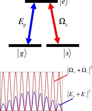
Figure 1: (color online) Schematic diagram of the three-level atomic system and the medium pumped by a standing wave coupling field.

The interaction Hamiltonian in rotating wave approximation reads

$$\hat{H}=-\hbar\sum_{j}\left(gE\hat{\sigma}_{eg}^{j}+\Omega_{c}\hat{\sigma}_{es}^{j}\right)+H.c.,$$ (1)

where $E$ is the dimensionless slowly-varying complex amplitude of the probe field, $g$ is the atom field coupling constant, $\Omega_{c}$ is the Rabi frequency of the coupling field, and $\hat{\sigma}_{\mu\nu}^{j}=\left|\mu\right\rangle_{jj}\left\langle\nu\right|$ are the atomic transition operators of the $j$th atom between states $|\mu\rangle$ and $|\nu\rangle$. The atom dynamics is governed by Langevin equations corresponding to (1) and including losses from the excited state. They can be written as

$$\partial_{t}\hat{\sigma}_{ge} = -\Gamma\hat{\sigma}_{ge}+igE(\hat{\sigma}_{gg}-\hat{\sigma}_{ee})+i\Omega_{c}\hat{\sigma}_{gs},$$ (2)

$$\partial_{t}\hat{\sigma}_{gs} = i\Omega_{c}^{\ast}\hat{\sigma}_{ge}+igE\hat{\sigma}_{es},$$ (3)

where $\Gamma$ is the relaxation rate of the upper level and it is assumed that the decoherence of the lower-level transition is negligible on the time scale of interest. In the limit of low probe-field intensities ($|gE|\ll|\Omega_{c}|$) and for an initial preparation of the ensemble in the ground state $|g\rangle$, we can set in eq.(2) $\hat{\sigma}_{gg}\approx\hat{1};\quad\hat{\sigma}_{ss}=\hat{\sigma}_{ee}=\hat{\sigma}_{se}=0$, which corresponds to the well-known pertubative linear-response limit. Since losses are included in the above equations there should be in general Langevin noise operators Gardiner . The noise operators are however inconsequential since in the linear-response limit, considered here, there is no excitation of the excited states. Thus they are neglected. We assume furthermore, that the characteristic duration of interaction $T$ is long compared with respect to the upper level relaxation ($\Gamma T\gg 1)$. This allows for an adiabatic elimination of the optical coherence $\hat{\sigma}_{ge}$ and equations (2) are reduced to

$$\Gamma\hat{\sigma}_{ge} =igE+i\Omega_{c}\hat{\sigma}_{gs}$$ (4)

$$\partial_{t}\hat{\sigma}_{gs} =i\Omega_{c}^{\ast}\hat{\sigma}_{ge}.$$

Differentiating the first equation with respect to time and assuming a constant control field $\Omega_{c}$ yields

$$\partial_{t}\hat{\sigma}_{ge}=\frac{ig}{\Gamma}\partial_{t}E-\frac{|\Omega_{c}|^{2}}{\Gamma}\hat{\sigma}_{ge},$$

which has the formal solution

$$\hat{\sigma}_{ge}\left(z,t\right) = \frac{ig}{\Gamma}\int\limits_{0}^{t}\frac{\partial E}{\partial\tau}\exp\left\{-\frac{|\Omega_{c}|^{2}}{\Gamma}(t-\tau)\right\}{\rm d}\tau$$ (5)

$$+i\frac{\Omega_{c}}{\Gamma}\hat{\sigma}_{gs}\left(z,0\right)\exp\left\{-\frac{|\Omega_{c}|^{2}}{\Gamma}t\right\}.$$

Since the coupling field is a standing wave formed by two counterpropagating fields of equal intensity and polarization, it can be expressed as $\Omega_{c}\left(z\right)=2\Omega\cos\left(kz\right)$, where $\Omega$ represents the amplitude of the coupling field. The probe field consists also of two counterpropagating components $E=E_{+}e^{ikz}+E_{-}e^{-ikz}$. Due to the presence of $|\Omega_{c}(z)|^{2}$ in the exponents in eq.5, the optical coherence and thus by virtue of eq.4 also the ground-state coherence will develop all harmonics of $e^{\pm ikz}$. Thus we make the ansatz

$$\hat{\sigma}_{gs}\left(z,t\right) = \sum\limits_{n=-\infty}^{\infty}\hat{\sigma}_{gs}^{(n)}\left(z,t\right)e^{iknz},$$ (6)

$$\hat{\sigma}_{ge}\left(z,t\right) = \sum\limits_{n=-\infty}^{\infty}\hat{\sigma}_{ge}^{(n)}\left(z,t\right)e^{iknz}.$$

The secular approximation corresponds to disregarding all terms in $\hat{\sigma}_{gs}$ with $n\neq 0$. This is justified in a hot gas where atomic motion washes out the fast spatial oscillations associated with terms $\hat{\sigma}_{gs}^{(n)}$ and $n\neq 0$ Andre-PRL-2002 ,Zimmer-OptComm-2006 .

The propagation of the probe pulse components are governed by the Maxwell equations for the slowly varying field amplitudes

$$\left(\frac{\partial}{\partial t}\pm c\frac{\partial}{\partial z}\right)E_{\pm}=igN\hat{\sigma}_{ge}^{(\pm 1)}.$$ (7)

where $\hat{\sigma}_{ge}^{(\pm 1)}$ are the components of atomic coherence between levels $\left|g\right\rangle$ and $\left|e\right\rangle$ that oscillate in space according to $e^{\pm ikz}$, and $N$ is the number density of atoms.

If the stationary light pulse is generated from a stored spin coherence without rapidly oscillating components, i.e. for $\sigma_{gs}^{(\pm n)}(z,t=0)=0$, for $n\neq 0$ the corresponding initial conditions are

$$\Gamma\hat{\sigma}_{ge}^{\pm 1}(z,0) = i\Omega\,\hat{\sigma}_{gs}(z,0),$$ (8)

$$\hat{\sigma}_{ge}^{\pm n}(z,0) = 0,\quad\text{for}\enspace n\neq 1.$$

Using the identity $e^{A\cos z}=\sum\limits_{n=-\infty}^{\infty}I_{\left|n\right|}\left(A\right)\cos\left(zn\right)=\sum\limits_{n=-\infty}^{\infty}I_{\left|n\right|}\left(A\right)\text{e}^{izn}$, with $I_{n}$ being the $n$th order modified Bessel function, we can rewrite equation (5).

$$\qquad\qquad\hat{\sigma}_{ge}^{(\pm 1)}=\frac{ig}{\Gamma}\,\int\limits_{0}^{t}\mathrm{d}t^{\prime}\,e^{-\beta(t-t^{\prime})}\times$$ (9)

$$\times\left[I_{0}\left(\beta(t-t^{\prime})\right)\frac{\partial E_{\pm}}{\partial t^{\prime}}-I_{1}\left(\beta(t-t^{\prime})\right)\frac{\partial E_{\mp}}{\partial t^{\prime}}\right]$$

$$\enspace+i\hat{\sigma}_{gs}(z,0)\Omega\mathrm{e}^{-\beta t}\left[I_{0}\Bigl{(}\beta t\Bigr{)}-I_{1}\Bigl{(}\beta t\Bigr{)}\right]/\Gamma,$$

where we have introduced $\beta=2\Omega^{2}/\Gamma$. If we consider times $t$ which are sufficiently large, the initial value term in eq.(9) can be disregarded.

Substituting (9) and (8) into equations (7) and introducing the sum and difference normal modes $E_{s}=E_{+}+E_{-}$, $E_{d}=E_{+}-E_{-}$ yields

$$\frac{\partial E_{s}}{\partial t}+c\frac{\partial E_{d}}{\partial z} =-\frac{g^{2}N}{\Gamma}\int\limits_{0}^{t}\mathrm{d}t^{\prime}f_{-}\Bigl{(}\beta(t-t^{\prime})\Bigr{)}\frac{\partial E_{s}}{\partial t^{\prime}}$$ (10)

$$\frac{\partial E_{d}}{\partial t}+c\frac{\partial E_{s}}{\partial z} =-\frac{g^{2}N}{\Gamma}\int\limits_{0}^{t}\mathrm{d}t^{\prime}f_{+}\Bigl{(}\beta(t-t^{\prime})\Bigr{)}\frac{\partial E_{d}}{\partial t^{\prime}},$$ (11)

where $f_{\pm}(x)=e^{-x}\Bigl{[}I_{0}\bigl{(}x\bigr{)}\pm I_{1}\bigl{(}x\bigr{)}\Bigr{]}$.

For the following discussion it is convenient to introduce normalized variables and parameter

$$\tau\equiv\frac{g^{2}N}{\Gamma}\,t,\qquad\xi\equiv\frac{z}{l_{\mathrm{abs}}},\qquad a\equiv\frac{2\Omega^{2}}{g^{2}N}=2\cot^{2}\theta,$$ (12)

where $l_{\mathrm{abs}}=c\Gamma/g^{2}N$ is the resonant absorption length of the medium in the absence of EIT. This leads to the normalized equations

$$\partial_{\tau}E_{s}+\partial_{\xi}E_{d} = -\int_{0}^{\tau}\!\!\mathrm{d}\tau^{\prime}\,f_{-}\bigl{(}a(\tau-\tau^{\prime})\bigr{)}\,\partial_{\tau^{\prime}}E_{s},$$ (13)

$$\partial_{\tau}E_{d}+\partial_{\xi}E_{s} = -\int_{0}^{\tau}\!\!\mathrm{d}\tau^{\prime}\,f_{+}\bigl{(}a(\tau-\tau^{\prime})\bigr{)}\,\partial_{\tau^{\prime}}E_{d}.$$ (14)

III probe-field dynamics

In the following we will qualitatively discuss the probe-field dynamics resulting from eqs.(13,14), illustrate the results with numerical examples and compare the field evolution with the case of a hot atomic gas. Eqs.(13,14) turn into the corresponding equations for a warm atomic gas where the secular approximation is valid, if one sets $f_{-}(a(\tau-\tau^{\prime}))\sim(2/a)\delta(\tau-\tau^{\prime})$, and $f_{+}(a(\tau-\tau^{\prime}))\to 1$

$$\frac{\partial E_{s}}{\partial\tau}+\frac{\partial E_{d}}{\partial\xi} = -\tan^{2}\theta\frac{\partial E_{s}}{\partial\tau},$$ (15)

$$\frac{\partial E_{d}}{\partial\tau}+\frac{\partial E_{s}}{\partial\xi} = -E_{d},$$ (16)

where $\tan^{2}\theta=g^{2}N/\Omega^{2}$. In this case adiabatic eliminating the fast decaying difference mode, i.e. $E_{d}\simeq-\partial_{\xi}E_{s}$, results in a diffusion equations for the sum mode

$$\frac{\partial E_{s}}{\partial\tau}+\frac{\partial^{2}E_{s}}{\partial\xi^{2}}=0,\qquad$$ (17)

$$\text{or}\qquad\frac{\partial E_{s}}{\partial t}+v_{\mathrm{gr}}l_{\mathrm{abs}}\frac{\partial^{2}E_{s}}{\partial z^{2}}=0,$$ (18)

where $v_{\mathrm{gr}}=c\cos^{2}\theta$ is the group velocity of EIT. Associated with the diffusion is a (non-exponential) loss of excitation with a characteristic time scale of $T_{\mathrm{loss}}^{s}={L^{2}}/{l_{\mathrm{abs}}v_{\mathrm{gr}}}$, with $L$ being the characteristic initial confinement length of the stationary pulse.

In order to discuss the stationary-light dynamics beyond the secular approximation we start with numerical solutions of eqs.(13,14) for two characteristic cases. In Fig.2 the decay of the total field intensity $I=\int\mathrm{d}z(E_{+}^{2}+E_{-}^{2})$ in the interval $\{-3L_{0},3L_{0}\}$ is shown after retrieval of an initial gaussian spin excitation of spatial shape $\exp\bigl{\{}-z^{2}/L_{0}^{2}\bigr{\}}$, and $L_{0}=5l_{\mathrm{abs}}$ (solid line) for two important cases. In the first case (top curve) $\tan^{2}\theta=100$, i.e. $a=0.02$, in the second (bottom curve) $\tan^{2}\theta=1$, i.e. $a=2$. Also shown is a comparision with the results obtained with the secular approximation (dotted line).

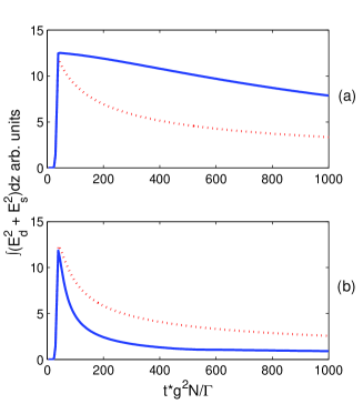
Figure 2: (color online) Decay of total field intensity within the spatial region from -3 $L_{0}$ to 3 $L_{0}$ for an initial spin excitation of spatial shape $\exp\{-z^{2}/L_{0}^{2}\}$, $L_{0}=5l_{\mathrm{abs}}$ in cold atomic gas (blue, solid line) and in inhomogeneously broadened (red, dotted line) media for $\tan^{2}\theta=100$ (top) and $\tan^{2}\theta=1$ (bottom).

The time evolution of the field distributions of $E_{s}$ and $E_{d}$ for the two cases are shown in Fig.3 ($\tan^{2}\theta=100$) and Fig.4 ($\tan^{2}\theta=1$).

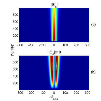
Figure 3: (color online) Spatio-temporal dynamics of sum $E_{s}$ (a) and difference $E_{d}\times 10$ (b) modes of the probe field corresponding to the top curve in Fig.2, i.e. $\tan^{2}\theta=100$.

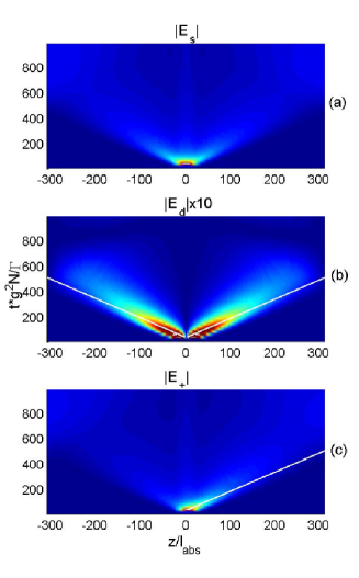
Figure 4: (color online) Spatio-temporal dynamics of sum $E_{s}$ (a) and difference $E_{d}\times 10$ (b) modes of the probe field, as well as field component $E_{+}$ (c), corresponding to the bottom curve in Fig.2, i.e. $\tan^{2}\theta=1$. The white lines indicate the velocity $2c\cos^{2}\theta/(2\cos^{2}\theta+\sin^{2}\theta)$.

From the numerical examples several conclusions can be drawn: First of all one recognizes that contrary to the claims in Ref.Molmer the field intensity decays even if the dephasing of the ground-state coherence is neglected. The decay is caused by the relaxation of the upper state which was not taken into account in Molmer by restricting the discussion to the loweest order in the adiabatic expansion. Thus stationary light in cold gases or solids does not provide a perfect cavity. Secondly the decay of the intensity can either be slower or faster as compared to the case with secular approximation. In the first case, i.e. Fig.3 the evolution of the field distribution is very similar to the diffusive spreading but much slower than in the secular-approximation limit shown in Fig.5. On the other hand in the second case (see Fig.4), two pulse components emerge which propagate with the group velocity $v_{\mathrm{gr}}=c\cos^{2}\theta$ with some additional loss Xue-PRA-2008 .

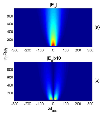
Figure 5: (color online) Dynamics of the sum $E_{s}$ (a) and difference modes $E_{d}\times 10$ (b) of the probe field in inhomogeneosly broadened medium, i.e. under conditions that justify the secular approximation. All parameteres are identical to the Fig.2.

We now want to give a qualititative explanation of the different dynamics in the two cases, which is due to the different action of the integral kernels $f_{\pm}$ in eqs.(13) and (14). For this it is instructive to perform a Laplace-transform of eqs.(13) and (14):

$$s\widetilde{E}_{s}-E_{s}(0)+\partial_{\xi}\widetilde{E}_{d} = -\widetilde{f}_{-}(s)\cdot\left(s\widetilde{E}_{s}-E_{s}(0)\right),$$ (19)

$$s\widetilde{E}_{d}-E_{d}(0)+\partial_{\xi}\widetilde{E}_{s} = -\widetilde{f}_{+}(s)\cdot\left(s\widetilde{E}_{d}-E_{d}(0)\right),$$ (20)

where the Laplace transform of $f_{\pm}$ reads

$${\widetilde{f}}_{+}(s) = \frac{1}{a}\left[\sqrt{2\frac{a}{s}+1}-1\right],$$

$${\widetilde{f}}_{-}(s) = \frac{1}{a}\left[-\frac{1}{\sqrt{2\frac{a}{s}+1}}+1\right].$$

This yields

$$s\widetilde{E}_{s}-E_{s}(0) = -\frac{\partial_{\xi}\widetilde{E}_{d}}{1+{\widetilde{f}}_{-}(s)},$$ (21)

$$s\widetilde{E}_{d}-E_{d}(0) = -\frac{\partial_{\xi}\widetilde{E}_{s}}{1+{\widetilde{f}}_{+}(s)}.$$ (22)

III.0.1 limit of small $a$

Assuming that $a$ is small, a series expansion of $1/(1+{\widetilde{f}}_{\pm}(s))$ yields

$$\frac{1}{1+{\widetilde{f}}_{\pm}(s)}\approx\frac{s}{s+1}$$

For the slow time evolution, i.e. for (physical) times large compared to $(g^{2}N/\Gamma)^{-1}$ only values of $s\ll 1$ are relevant, and thus the right hand side can be replaced by $s$. Substituting this into eqs.(19) and (20) one arrives at

$$\partial_{\xi}^{2}E_{s}-E_{s} = -\left(E_{s}(\xi,0)+\partial_{\xi}E_{d}(\xi,0)\right),$$

$$\partial_{\xi}^{2}E_{d}-E_{d} = -\left(E_{d}(\xi,0)+\partial_{\xi}E_{s}(\xi,0)\right),$$

which describes truly stationary wave packets that decay exponentially with increasing distance. That there is no dynamics is of course due to the fact that only the leading order term in the expansion of $1/(1+{\widetilde{f}}_{\pm})$ was taken into account.

III.0.2 limit of large $a$

A qualitative explanation of the opposite case can be found by considering the limit of large $a$. To properly analyze this case one has to take into account that also the most relevant Laplace frequency $s$ increases when $a$ becomes large. In fact the numerical data suggest that the ratio $a/s$, with $s$ being the most relevant Laplace frequency approaches a constant. Thus in this case one has

$$\frac{1}{1+{\widetilde{f}}_{+}(s)} \approx \frac{a}{a-1+x}$$

$$\frac{1}{1+{\widetilde{f}}_{-}(s)} \approx \frac{a}{a+1-1/x},$$

where $x=\sqrt{2\dfrac{a}{s}+1}$ is well approximated by a constant. This leads to the approximate equations

$$\partial_{\tau}E_{s}+\frac{a}{a+1-1/x}\partial_{\xi}E_{d} = 0,$$

$$\partial_{\tau}E_{d}+\frac{a}{a-1+x}\partial_{\xi}E_{s} = 0.$$

In the limit of large $a\,$ one arrives at wave equations for the forward and backward components

$$\partial_{\tau}^{2}E_{\pm}{\pm}\frac{a^{2}}{(a+1-1/x)(a-1+x)}\partial_{\xi}^{2}E_{\pm}=0,$$

which reads in physical time and space:

$$\partial_{t}^{2}E_{\pm}{\pm}\frac{c^{2}a^{2}}{(a+1-1/x)(a-1+x)}\partial_{z}^{2}E_{\pm}=0.$$

Thus the envelope of $E_{\pm}$ evolves freely This explains the splitting of the stationary light wavepacket into two components each of which propagating with the modified group velocity $2c\cos^{2}\theta/(2\cos^{2}\theta+f\sin^{2}\theta)$, with $f=(x-1/x)/4$. Noting that the most relevant Laplace frequency for the example in Fig.4 leads to a value of $f$ on the order of unity we find reasonable agreement with the numerical results.

IV summary

We considered the dynamics of stationary light in a standing medium without secular approximation and derived equations describing the evolution of the sum and difference modes of the pulse. A numerical as well as approximate analytical solution showed that for small coupling field intensities the probe field spreading is slower than in the secular approximation but in contrast to the results of Molmer non-zero. In the opposite limit of strong coupling the probe pulse splits into two counterpropagating components.

G.N. acknowledges support by the Alexander von Humboldt Foundation.

References

- (1) J.H. Kimble, Phys. Scr. T 76, 127 (1998). J.M. Raimond, M. Brune, S. Haroche, Rev. Mod. Phys. 73, 565 (2001). H. Walther, B.T.H. Varcoe, B.G. Englert and Th. Becker, Rep. Prog. Phys. 69, 1325 (2006).
- (2) A. Andre and M.D. Lukin, Phys. Rev. Lett. 89, 143602 (2002); A. Andre, M. Bajcsy, A.S. Zibrov, and M.D. Lukin, Phys. Rev. Lett. 94, 063902 (2005).
- (3) M. Bajcsy, A. S. Zibrov, M.D. Lukin, Nature (London), 426, 638 (2003).
- (4) S. E. Harris, Physics Today, 50, Nr.7, 36 (1997).
- (5) M. Fleischhauer, A. Imamoglu, and J. P. Marangos, Rev. Mod. Phys. 77, 663 (2005).
- (6) F. E. Zimmer, A. Andre, M. D. Lukin, and M. Fleischhauer, Opt. Comm. 264, 441 (2006)
- (7) F. E. Zimmer, J. Otterbach, R. G. Unanyan, B. W. Shore and M. Fleischhauer, Phys. Rev. A 77, 063823 (2008); Y. D. Chong, and M. Soljacic, Phys. Rev. A 77, 013823 (2008).
- (8) J. Otterbach, R.G. Unanyan and M. Fleischhauer, Phys. Rev. Lett. 102, 063602 (2009).
- (9) D. E. Chang, V. Gritsev, G. Morigi, V. Vuleti, M. D. Lukin, E. A. Demler, Nature Physics 4, 884 (2008).
- (10) M. Fleischhauer, J. Otterbach, and R.G. Unanyan, Phys. Rev. Lett. 101, 163601 (2008).
- (11) A. V. Turukhin, V. S. Sudarshanam, M. S. Shahriar, J. A. Musser, B. S. Ham, and P. R. Hemmer, Phys. Rev. Lett. 88, 023602 (2001).
- (12) M. Masalas and M. Fleischhauer, Phys. Rev. A 69, 061801(R) (2004).
- (13) F. Gerbier, S. Trotzky, S. Folling, U. Schnorrberger, J. D. Thompson, A. Widera, I. Bloch, L. Pollet, M. Troyer, B. Capogrosso-Sansone, N. V. Prokof’ev, B. V. Svistunov, Phys. Rev. Lett. 101, 155303 (2008).
- (14) S.A. Moiseev and B.S. Ham, Phys. Rev. A 73, 033812 (2006).
- (15) S.A. Moiseev and B.S. Ham, Phys. Rev. A 71, 053802 (2005).
- (16) K.R. Hansen and K. Mølmer, Phys. Rev. A 75, 065804 (2007). K.R. Hansen and K. Mølmer, Phys. Rev. A 75, 053802 (2007).
- (17) Yan Xue and B. S. Ham, Phys. Rev. A 78, 053830 (2008).
- (18) Quantum Noise, C.W. Gardiner, P. Zoller, (Springer, Berlin, 2000).