ITEP-TH-11/09
LPTENS-09/05
UUITP-08/09

1 Introduction

A new example of the $AdS_{4}/CFT_{3}$ duality proposed in [2] and further developed in [3] establishes an equivalence of the superconformal Chern-Simons-matter theory and type IIA string theory on $AdS_{4}\times CP^{3}$ [4, 5, 6]. This AdS/CFT system turns out to be integrable [7, 4, 5, 8] and exactly solvable [9, 1, 10] in the large-$N$ (free string) limit. However, certain features of the available exact solution are rather puzzling and call for an explanation. The purpose of this paper is to address these puzzles and to clarify how the building blocks of the exact solution fit together with the perturbative spectrum of the string sigma-model.

Let us begin by shortly describing the exact solution of the planar $AdS_{4}/CFT_{3}$ system [10] from the worldsheet perspective, which is most appropriate for our purposes. An alternative but equivalent interpretation can be given in terms of an integrable spin chain that arises in the $\mathcal{N}=6$ Chern-Simons theory [7, 11, 12, 13, 14, 15]. The solution of [10] describes the exact spectrum of the string sigma-model in the light-cone gauge, which is a massive two-dimensional integrable quantum field theory. The main building blocks of the exact solution are the spectrum of elementary excitations and their exact S-matrix [1]. The S-matrix, defined on an infinitely long string, can be diagonalized by the Bethe ansatz equations [9]. The periodic boundary conditions of the closed string are then imposed with the help of the Y-system and thermodynamic Bethe ansatz [10].

The global symmetries, along with integrability, are of central importance for this construction. The global symmetry group of the string sigma-model on $AdS_{4}\times CP^{3}$ is $OSp(6|4)$, but in the light-cone gauge only the $PSU(2|2)\times U(1)$ subgroup is linearly realized. The worldsheet spectrum consists of massive particles, which transform in the $(2|2)_{+1}$ and $(2|2)_{-1}$ representations of $PSU(2|2)\times U(1)$ and have the dispersion relation [11]:

$$\varepsilon(p)=\sqrt{\frac{1}{4}+4h^{2}(\lambda)\sin^{2}\frac{p}{\sqrt{2\lambda}}}\,\,\stackrel{{\scriptstyle\lambda\rightarrow\infty}}{{\longrightarrow}}\,\,\sqrt{p^{2}+\frac{1}{4}}\,.$$ (1.1)

Here $\lambda$ is the ’t Hooft coupling of the Chern-Simons theory. The string tension is given by $T=\sqrt{\lambda/2}$ [2]. $h(\lambda)$ is an interpolating function [11] which behaves as $h(\lambda)\simeq\sqrt{\lambda/2}$ at strong coupling. At finite $p$ and $\varepsilon$ the elementary excitations are transverse fluctuations of the string moving on the light-like geodesic (the BMN modes) [17, 11, 4, 18]. If one pumps momentum $p\sim\sqrt{\lambda}$ in a BMN mode, it blows up into a soliton (the giant magnon) [11, 18, 19, 20, 21, 22, 23, 24, 25, 26, 27, 28, 29]. The factorizable scattering matrix of the solitons was constructed in [1] and is built from the Beisert’s $PSU(2|2)$-invariant S-matrix [30, 31] and the BES/BHL dressing phase [32, 33].

This picture has two puzzling features. Firstly, the soliton-antisoliton scattering according to [1] is completely reflectionless. This does not contradict any basic principles, but does not follow from the known symmetries either. In fact, different factorizable S-matrices with the same symmetries do exist, and have a non-vanishing reflection amplitude [34]. These S-matrices, however, disagree with explicit two-loop computations in the Chern-Simons theory [35]. Secondly, the number of degrees of freedom in the scattering theory and on the worldsheet do not match. The scattering theory of [1] describes $(2|2)+(2|2)=(4|4)$ worldsheet degrees of freedom, while critical superstring should have $(8|8)$. Indeed, fixing the light-cone gauge in the sigma-model (or, alternatively, expanding near a non-trivial spinning string solution [36, 37, 38, 39, 40]), one finds sixteen massive oscillation modes. Those include, in addition to the light modes (1.1), $(4|4)$ heavy modes with the dispersion [17, 11, 18]

$$E(p)=\sqrt{p^{2}+1}\,.$$ (1.2)

An interpretation of these modes is rather unclear. They do not show up in the scattering theory. Does this mean that the S-matrix is incomplete and has to be extended to a larger set of elementary excitations? The classical, large-$\lambda$ limit of the Bethe equations [8] suggests that this is not the case. As shown in [8], all sixteen BMN modes can be identified as solutions to the classical string Bethe equations. However, the solutions associated with the light and heavy modes are qualitatively different. While the light modes are associated with solitary Bethe roots, the heavy modes are described by stacks [8]. The stacks [41, 42] are compounds of two momentum-carrying Bethe roots, which are not bound states of the corresponding particles. Stacks can be identified only at extreme values of some small parameter, in this case the inverse string tension $2/\sqrt{2\lambda}$. At finite $\lambda$, a stack is indistinguishable from a generic two-particle state.

We suggest the following resolution of the apparent mismatch in the number of degrees of freedom. In order to understand if the heavy modes exist as elementary excitations, we need to see whether they appear as poles in Green’s functions or not. Let us consider the propagator of a heavy mode $G(\omega,p)$. At strictly infinite coupling it has a pole at $\omega=E(p)$. We are going to argue, however, that $\alpha^{\prime}$ corrections cannot be neglected even if the coupling $1/\sqrt{2\lambda}$ is very small. The reason is that the pole lies exactly at the threshold of pair production of two light modes. The polarization operator thus has a cut with the branch point also at $\omega=E(p)$: $\Pi(\omega,p)\sim i(\omega-E(p))^{\nu}$. For the $\Phi\phi^{2}$-type interaction in two dimensions, we would expect $\nu=-1/2$, but as we shall see later the derivatives in the heavy-light-light interaction vertex soften the threshold singularity to $\nu=+1/2$. The one-loop corrected Green’s function thus behaves near the threshold as

$$G(\omega,p)\sim\frac{iZ(p)}{\omega-E(p)+\frac{C(p)}{\sqrt{2\lambda}}\,\sqrt{E(p)-\omega}}\,.$$ (1.3)

Sufficiently close to $E(p)$, for $|\omega-E(p)|\sim 1/\lambda$, the second term in the denominator is as important as the first one and can change the analytic properties of $G(\omega,p)$. Whether the pole in $G(\omega,p)$ survives or not depends on the sign of $C$. If $C$ is positive, the pole shifts below the threshold: $E_{\rm 1-loop}=E-C^{2}/2\lambda$. If $C$ is negative, the pole disappears. The propagator then has only a cut on the physical sheet which means that the heavy mode dissolves in the continuum and does not exist as a physical excitation at finite $\lambda$.

We will calculate the polarization operator for one of the heavy modes (the others should be related by supersymmetry) using the large-$\lambda$ (near-BMN) expansion of the sigma-model in $AdS_{4}\times CP^{3}$ [43, 44]. In [43, 44], the near-BMN expansion was utilized to compute energy shifts of the BMN oscillator spectrum. In these calculations the heavy modes were integrated out. The agreement of the near-BMN calculations with the Bethe-ansatz predictions [43, 44] implies that a contribution of the heavy modes is already contained in the S-matrix of [1]. We will compute the worldsheet S-matrix explicitly and in particular will verify that the reflection amplitude in the particle-antiparticle scattering cancels out to the leading order is the $1/\sqrt{\lambda}$ expansion.

2 The sigma-model

We will start with the supercoset formulation of the worldsheet sigma-model on $AdS_{4}\times{C}P^{3}$ [4, 5, 45], which arises after partially fixing kappa-symmetry gauge in the full Green-Schwarz action [6]. The construction of the supercoset $OSp(6|4)/SO(3,1)\times U(3)$ sigma-model is based on the $\mathbbm{Z}_{4}$ decomposition of the $osp(6|4)$ superalgebra:

$$osp(6|4)=h_{0}\oplus h_{1}\oplus h_{2}\oplus h_{3}.$$ (2.1)

Since the superalgebra admits a $\mathbb{Z}_{4}$ automorphism [4, 5], this decomposition is consistent with the (anti)commutation relations: $[h_{i},h_{j}\}\subset h_{(i+j)\!\!\mod\!4}$. The $h_{0}$ subalgebra is the denominator of the coset: $h_{0}=so(3,1)\oplus u(3)$, $h_{0}\oplus h_{2}$ is the bosonic subalgebra $so(3,2)\oplus su(4)$, and $h_{1}$, $h_{3}$ contain all the odd generators. The worldsheet embedding coordinates are parameterized by a coset representative $g(x)\in OSp(6|4)$, defined up to gauge transformations $g(x)\rightarrow g(x)h(x)$ with $h(x)\in SO(3,1)\times U(3)$. The global $OSp(6|4)$ acts from the left: $g(x)\rightarrow g^{\prime}g(x)$. The sigma-model action can be expressed in terms of the $OSp(6|4)$-invariant current

$$P_{\mu}=g^{-1}\partial_{\mu}g=P_{0\,\mu}+P_{1\,\mu}+P_{2\,\mu}+P_{3\,\mu}.$$ (2.2)

The $h_{0}$ component of the $\mathbbm{Z}_{4}$ decomposition of $P_{\mu}$ transforms as a gauge connection: $P_{0\,\mu}\rightarrow h^{-1}P_{0\,\mu}h+h^{-1}\partial_{\mu}h$. The other three components transform homogeneously: $P_{1,2,3\,\mu}\rightarrow h^{-1}P_{1,2,3\,\mu}h$. The Lagrangian of the sigma-model is

$$\mathcal{L}=\frac{\sqrt{2\lambda}}{2}\,\mathop{\mathrm{Str}}\left(\sqrt{-h}h^{\mu\nu}P_{2\,\mu}P_{2\,\nu}+\epsilon^{\mu\nu}P_{1\,\mu}P_{3\,\nu}\right),$$ (2.3)

where $\mathop{\mathrm{Str}}(\cdot\,\,\cdot)$ is the invariant bilinear form on $osp(6|4)$.

The light-cone gauge breaks $OSp(6|4)$ down to $PSU(2|2)\times U(1)$, of which only the bosonic subgroup $SU(2)\times SU(2)\times U(1)$ will be manifest. This suggests the following choice of basis in $osp(6|4)$:

$$h_{0} = \{R^{a}_{b},R^{a},R_{a},R;K_{i},T_{i}\}$$

$$h_{2} = \{B^{a},B_{a},J,M;L_{i},D\}$$

$$h_{1} = \{Q^{a}_{\alpha},\bar{Q}_{a\alpha},Q_{\alpha},\bar{Q}_{\alpha}\}$$

$$h_{3} = \{S_{a\alpha},\bar{S}^{a}_{\alpha},S_{\alpha},\bar{S}_{\alpha}\},$$ (2.4)

where $a,b=1,2$ and $\alpha=1,2$ are the indices of the unbroken $SU(2)\times SU(2)$. The commutation relations of $osp(6|4)$ are listed in appendix A, along with the components of the invariant bilinear form. The light-cone coordinates in the coset are conjugate to $D\pm iJ/2$. The unbroken subalgebra $su(2)\oplus su(2)\oplus u(1)$ is the set of generators that commute with both $J$ and $D$: $\{R^{a}_{b}-\delta^{a}_{b}R^{c}_{c}/2,R;T_{i}\}$. In the limit of an infinitely long string, which we will take later, the supercharges that commute with the light-cone Hamiltonian $D-iJ/2$ are also conserved. Those are $Q^{a}_{\alpha}-i\varepsilon^{ab}\bar{Q}_{b\alpha}$ and $\bar{S}^{a}_{\alpha}+i\varepsilon^{ab}S_{b\alpha}$. Together with the conserved bosonic generators they form a $psu(2|2)$ subalgebra.

In order to fix the light-cone gauge, it is convenient to use the following parameterization of the coset representative:

$$g=\,{\rm e}\,^{\Xi}\,{\rm e}\,^{\mathbbm{X}},$$ (2.5)

where

$$\Xi=tD+\frac{i}{2}\,\varphi J$$ (2.6)

and

$$\mathbbm{X} = \frac{1}{\sqrt{2}}\,X^{a}B_{a}+\frac{1}{\sqrt{2}}\,\bar{X}_{a}B^{a}+\frac{1}{2}\,ZM+Y^{i}L_{i}+\frac{1}{2}\,\varepsilon^{\alpha\beta}\varepsilon_{ab}\chi^{a}_{R\,\alpha}Q^{b}_{\beta}+\frac{i}{2}\,\varepsilon^{\alpha\beta}\chi^{a}_{R\,\alpha}\bar{Q}_{a\beta}$$ (2.7)

$$-i\bar{\psi}^{\alpha}_{L}Q_{\alpha}+i\varepsilon^{\alpha\beta}\psi_{R\,\alpha}\bar{Q}_{\beta}-\frac{1}{2}\,\varepsilon^{\alpha\beta}\chi^{a}_{L\,\alpha}S_{a\beta}-\frac{i}{2}\,\varepsilon^{\alpha\beta}\varepsilon_{ab}\chi^{a}_{L\,\alpha}\bar{S}^{b}_{\beta}-\varepsilon^{\alpha\beta}\psi_{L\,\alpha}S_{\beta}+\bar{\psi}^{\alpha}_{R}\bar{S}_{\alpha}.$$

By choosing the same coefficients in front of $Q^{a}_{\alpha}$, $\bar{Q}_{a\alpha}$ and $S_{a\alpha}$, $\bar{S}^{a}_{\alpha}$, we eliminate eight fermionic degrees of freedom and thus fix the residual kappa-symmetry [4] of the coset sigma-model.

The light-cone gauge treats $t$, $\varphi$ and the rest of the world-sheet coordinates asymmetrically. The centre of mass of the string moves along the light-like geodesic $\varphi=t$, and we need to keep the dependence on $t$ and $\varphi$ in the Lagrangian exactly. The string oscillations in the transverse directions, which are parameterized by $\mathbbm{X}$, are small and can be treated perturbatively. The current (2.2) expands as

$$P_{\mu}=\partial_{\mu}\Xi+\frac{1-\,{\rm e}\,^{-\mathop{\mathrm{ad}}\mathbbm{X}}}{\mathop{\mathrm{ad}}\mathbbm{X}}\,\mathcal{D}_{\mu}\mathbbm{X}=\partial_{\mu}\Xi+\mathcal{D}_{\mu}\mathbbm{X}-\frac{1}{2}[\mathbbm{X},\mathcal{D}_{\mu}\mathbbm{X}]+\frac{1}{6}[\mathbbm{X},[\mathbbm{X},\mathcal{D}_{\mu}\mathbbm{X}]]+\ldots.$$ (2.8)

where the long derivative is defined by

$$\mathcal{D}_{\mu}\mathbbm{X}=\partial_{\mu}\mathbbm{X}+[\partial_{\mu}\Xi,\mathbbm{X}].$$ (2.9)

Plugging this expansion into the Lagrangian (2.3) one can get the sigma-model action to any desired order in $\mathbbm{X}$, although explicit expressions quickly get complicated.

To the two lowest orders, and omitting the overall factors of $\sqrt{\lambda/2}$ and $\sqrt{-h}$,

$$\mathcal{L}^{(0)}=\frac{1}{2}\left(\partial_{\mu}\varphi\right)^{2}-\frac{1}{2}\left(\partial_{\mu}t\right)^{2},$$ (2.10)

and

$$\mathcal{L}^{(2)} = \partial_{\mu}\bar{X}_{a}\partial^{\mu}X^{a}+\frac{1}{2}\left(\partial_{\mu}Z\right)^{2}+\frac{1}{2}\left(\partial_{\mu}Y_{i}\right)^{2}$$ (2.11)

$$+i\bar{\psi}^{\alpha}\gamma^{\mu}\overleftrightarrow{\partial_{\nu}}\psi_{\alpha}\Pi_{\mu}^{\nu\lambda}\partial_{\lambda}t+\frac{i}{4}\,\bar{\chi}^{\alpha}_{a}\gamma^{\mu}\overleftrightarrow{\partial_{\nu}}\chi^{a}_{\alpha}\Pi_{\mu}^{\nu\lambda}\partial_{\lambda}\left(t+\varphi\right)$$

$$-\left(\frac{1}{2}\,Y^{2}_{i}+\frac{1}{2}\,\bar{\psi}^{\alpha}\psi_{\alpha}+\frac{1}{8}\,\bar{\chi}^{\alpha}_{a}\chi^{a}_{\alpha}\right)\left(\partial_{\mu}t\right)^{2}-\left(\frac{1}{2}\,Z^{2}+\frac{1}{4}\,\bar{X}_{a}X^{a}+\frac{1}{8}\,\bar{\chi}^{\alpha}_{a}\chi_{\alpha}^{a}\right)\left(\partial_{\mu}\varphi\right)^{2}$$

$$-\frac{1}{4}\,\bar{\chi}^{\alpha}_{a}\chi_{\alpha}^{a}\partial_{\mu}t\partial^{\mu}\varphi-\frac{1}{8}\,\bar{\chi}^{\alpha}_{a}\chi_{\alpha}^{a}\epsilon^{\mu\nu}\partial_{\mu}t\partial_{\nu}\varphi,$$

where the fermions have been combined into two-dimensional Dirac ($\psi_{\alpha}$) and Majorana ($\chi_{\alpha}^{a}$) spinors:

$$\psi_{\alpha}=\begin{pmatrix}\psi_{L\,\alpha}\\ \psi_{R\,\alpha}\\ \end{pmatrix}, \bar{\psi}^{\alpha}=\left(\bar{\psi}_{L}^{\alpha}\,\,\,\bar{\psi}_{R}^{\alpha}\right)$$ (2.12)

$$\chi^{a}_{\alpha}=\begin{pmatrix}\chi^{a}_{L\,\alpha}\\ \chi^{a}_{R\,\alpha}\\ \end{pmatrix}, \bar{\chi}^{\alpha}_{a}=-i\varepsilon^{\alpha\beta}\varepsilon_{ab}\left(-\chi^{b}_{R\,\beta}\,\,\,\chi^{b}_{L\,\beta}\right)=-i\varepsilon^{\alpha\beta}\varepsilon_{ab}\chi^{b\,T}_{\beta}\gamma^{1}.$$ (2.13)

The Dirac matrices $\gamma^{\mu}$ are chosen to be

$$\gamma^{\mu}=(\sigma^{1},i\sigma^{2}).$$ (2.14)

The symbol $\Pi_{\mu}^{\nu\lambda}$ is defined as

$$\Pi_{\mu}^{\nu\lambda}=\delta_{\mu}^{0}h^{\nu\lambda}+\frac{1}{\sqrt{-h}}\,\delta^{1}_{\mu}\epsilon^{\nu\lambda}.$$ (2.15)

Fixing the light-cone gauge at the quadratic level in fluctuations amounts to treating $t$ and $\varphi$ as classical background fields: $t=\tau=\varphi$ and replacing $h^{\mu\nu}$ by the flat Minkowski metric $\eta_{\mu\nu}$. Then $\partial_{\mu}t=\delta^{0}_{\mu}=\partial_{\mu}\varphi$, $\Pi^{\nu 0}_{\mu}=\delta^{\nu}_{\mu}$, and (2.11) becomes

$$\mathcal{L}^{(2)}_{\rm g.f.} = \partial_{\mu}\bar{X}_{a}\partial^{\mu}X^{a}-\frac{1}{4}\,\bar{X}_{a}X^{a}+\frac{1}{2}\left(\partial_{\mu}Z\right)^{2}-\frac{1}{2}\,Z^{2}+\frac{1}{2}\left(\partial_{\mu}Y_{i}\right)^{2}-\frac{1}{2}\,Y^{2}_{i}$$ (2.16)

$$+i\bar{\psi}^{\alpha}\gamma^{\mu}\partial_{\mu}\psi_{\alpha}-\frac{1}{2}\bar{\psi}^{\alpha}\psi_{\alpha}+\frac{i}{2}\,\bar{\chi}^{\alpha}_{a}\gamma^{\mu}\partial_{\mu}\chi^{a}_{\alpha}-\frac{1}{2}\,\bar{\chi}^{\alpha}_{a}\chi^{a}_{\alpha}.$$

This Lagrangian describes two complex scalars and two Dirac fermions of mass $1/2$, and four real scalars and four Majorana fermions of mass $1$ (the second equation in (2.13) can be regarded as a Majorana condition). The Lagrangian is equivalent to the one derived in [4], although we have used a different coset parameterization. The light modes $(X^{a},\psi_{\alpha})$, $(\bar{X}_{a},\bar{\psi}^{\alpha})$ correspond to particles and anti-particles of the worldsheet scattering theory and transform in the $(2|2)_{\pm 1}$ representations of the unbroken symmetry group $PSU(2|2)\times U(1)$. The heavy modes $(Z,Y_{i},\chi^{a}_{\alpha})$ are neutral under $U(1)$ and transform in the $(\mathbf{1},\mathbf{1})$, $(\mathbf{1},\mathbf{3})$ and $(\mathbf{2},\mathbf{2})$ representations of $SU(2)\times SU(2)$.

Higher orders of the expansion in $\mathbb{X}$ describe interactions of the BMN modes, which will lead to non-trivial scattering and to quantum corrections. Our goal will be to compute the imaginary part of the polarization operator for the $Z$ field at one loop and the $2\rightarrow 2$ scattering amplitudes for $X^{a}$ and $\bar{X}_{a}$ at the tree level. For that we need to expand the sigma-model Lagrangian to the quartic order in fluctuations. The resulting general expressions are quite complicated, but for this particular computation only a few terms are necessary. These terms in fact are quite simple. At the cubic level, the interaction terms that involve $Z$ and two light fields are generally of the form $Z\bar{\psi}\psi$ and $Z\bar{X}X$. In the parameterization (2.7) the $Z\bar{\psi}\psi$ vertex is absent, and we are left with the unique $Z\bar{X}X$ term:

$$\mathcal{L}^{(3)}=i\,Z\bar{X}_{a}\overleftrightarrow{\partial_{\mu}}X^{a}\partial^{\mu}\varphi+\ldots.$$ (2.17)

Again, the gauge fixing amounts to replacing $\partial_{\mu}\varphi$ by $\delta_{\mu}^{0}$ and $h^{\mu\nu}$ by the Minkowski metric (see appendix B for a more rigorous argument):

$$\mathcal{L}^{(3)}_{\rm g.f.}=iZ\bar{X}_{a}\overleftrightarrow{\partial_{0}}X^{a}+\ldots.$$ (2.18)

At the quartic level the only terms we need are the $X$, $\bar{X}$ self-interactions:

$$\mathcal{L}^{(4)} = \frac{1}{24}\left(\bar{X}_{a}X^{a}\right)^{2}\left(\partial_{\mu}\varphi\right)^{2}+\frac{1}{6}\left(\partial_{\mu}\bar{X}_{a}X^{a}\right)^{2}+\frac{1}{6}\left(\bar{X}_{a}\partial_{\mu}X^{a}\right)^{2}-\frac{1}{6}\,\bar{X}_{a}\partial_{\mu}X^{a}\partial^{\mu}\bar{X}_{b}X^{b}$$ (2.19)

$$-\frac{1}{6}\,\partial_{\mu}\bar{X}_{a}\partial^{\mu}X^{a}\bar{X}_{b}X^{b}+\ldots.$$

Applying the gauge-fixing procedure outlined in appendix B to the Lagrangian (2.10), (2.11), (2.17), (2.19) we get

$$\mathcal{L}^{(4)}_{\rm g.f.} = \frac{6a-5}{96}\left(\bar{X}_{a}X^{a}\right)^{2}+\frac{1}{6}\left(\partial_{\mu}\bar{X}_{a}X^{a}\right)^{2}+\frac{1}{6}\left(\bar{X}_{a}\partial_{\mu}X^{a}\right)^{2}-\frac{1}{6}\,\bar{X}_{a}\partial_{\mu}X^{a}\partial^{\mu}\bar{X}_{b}X^{b}$$ (2.20)

$$-\frac{1}{6}\,\partial_{\mu}\bar{X}_{a}\partial^{\mu}X^{a}\bar{X}_{b}X^{b}-\frac{1-2a}{2}\left(\partial_{\mu}\bar{X}_{a}\partial^{\mu}X^{a}\right)^{2}$$

$$+\frac{1-2a}{4}\left(\partial_{\mu}\bar{X}_{a}\partial_{\nu}X^{a}+\partial_{\nu}\bar{X}_{a}\partial_{\mu}X^{a}\right)^{2}+\frac{1}{4}\,\bar{X}_{a}X^{a}\left(\partial_{0}\bar{X}_{b}\partial_{0}X^{b}+\partial_{1}\bar{X}_{b}\partial_{1}X^{b}\right)+\ldots\!,$$

where $a$ is the gauge-fixing parameter, $0\leqslant a\leqslant 1/2$, which interpolates between the temporal gauge ($a=0$) and the pure light-cone gauge ($a=1/2$) [46]. The gauge-fixed string action is

$$S_{\rm l.c.}=\frac{\sqrt{2\lambda}}{2}\int d^{2}x\,\left(\mathcal{L}^{(2)}_{\rm g.f.}+\mathcal{L}^{(3)}_{\rm g.f.}+\mathcal{L}^{(4)}_{\rm g.f.}+\ldots\right),$$ (2.21)

where the fields are periodic in $x^{1}$ with the period $\mathcal{J}_{+}=2[(1-a)J+aE]/\sqrt{2\lambda}$ (appendix B). We will ignore this periodicity by sending $\mathcal{J}_{+}$ to infinity, and will treat (2.21) as a massive two-dimensional field theory on a plane with the coupling constant $\sqrt{2\lambda}/2$.

Our gauge-fixed Lagrangian is different from those in [43] and [44], where different sets of coordinates on $CP^{3}$ were used. The Lagrangians should be related by field redefinitions. In the next two sections we will use the light-cone string Lagrangian to compute the one-loop polarization operator for $Z$, and the tree level scattering matrix for $X$, $\bar{X}$.

3 Quantum corrections for the heavy mode

Figure 1: The one-loop self-energy graphs.

There are two types of diagrams that contribute to the self-energy of $Z$ at one loop (fig. 1). In principle all cubic and quartic vertices that involve $Z$ are necessary to compute the one-loop polarization operator, but only the heavy-light-light vertex contributes to the threshold singularity at $\omega=E(p)$ we are interested in. Indeed, the bubble graph, fig. 1b, does not have an imaginary part, and the two-particle cut of the diagram 1a with a heavy mode in the loop starts at $\omega=2E(p/2)$ rather than at $\omega=E(p)=2\varepsilon(p/2)$.

Since $Z$ couples to the charge density of $X$, the polarization operator $\Pi(\omega,p)$ can be expressed through the $00$ component of the correlator of currents:

$$\Pi=\frac{2}{\sqrt{2\lambda}}\,\Pi_{00},$$ (3.1)

where

$$\Pi_{\mu\nu}=i\int d^{2}x\,\,{\rm e}\,^{-i\vec{p}\vec{x}}\left\langle J_{\mu}(x)J_{\nu}(0)\right\rangle,\qquad J_{\mu}=i\bar{X}_{a}\overleftrightarrow{\partial_{\mu}}X^{a}.$$ (3.2)

The standard Feynman parameter representation for the loop integral gives

$$\Pi_{\mu\nu}=\frac{1}{8\pi}\left\{\frac{2}{\varepsilon}-\gamma+\ln(4\pi)+\int_{0}^{1}dx\,\left[2\eta_{\mu\nu}\ln\left(\frac{1}{4}-x(1-x)\vec{p}^{\,2}\right)+\frac{(1-2x)^{2}p_{\mu}p_{\nu}}{\frac{1}{4}-x(1-x)\vec{p}^{\,2}}\right]\right\},$$ (3.3)

where we have used dimensional regularization to cut off the divergence. The divergent term does not contribute to $\mathop{\mathrm{Im}}\Pi$ and should cancel against the bubble graph 1b plus the heavy mode loop in 1a.

Near the threshold ($\vec{p}^{\,2}=1$):

$$\mathop{\mathrm{Im}}\Pi_{\mu\nu}\simeq-\frac{1}{4}\,\left(p_{\mu}p_{\nu}-\eta_{\mu\nu}\right)\sqrt{1-\vec{p}^{\,2}}\,,$$ (3.4)

and

$$\mathop{\mathrm{Im}}\Pi(\omega,p)\simeq-\frac{\sqrt{2E(p)}}{2\sqrt{2\lambda}}\,p^{2}\sqrt{E(p)-\omega}\,.$$ (3.5)

The function $C$ in (1.3) thus is given by

$$C(p)=-\frac{p^{2}}{2\sqrt{2E(p)}}\,,$$ (3.6)

and is strictly negative. From the discussion following eq. (1.3) we conclude that the one-particle pole in the $Z$ propagator disappears once quantum corrections are taken into account. There is no world-sheet particle associated with $Z$, it dissolves in the $X$–$\bar{X}$ continuum. We expect the same to happen with the other heavy modes, by supersymmetry. Indeed, there are terms of the form $Y_{i}\bar{\psi}^{\alpha}\sigma_{i\alpha}^{\hphantom{i\alpha}\beta}\psi_{\beta}$ and $\bar{\chi}^{\alpha}_{a}\psi_{\alpha}\bar{X}_{b}\varepsilon^{ab}$ in the cubic Lagrangian that can mediate the mixing of $Y_{i}$ and $\chi_{\alpha}^{a}$ with the light modes. Strictly speaking the conclusion that the heavy modes dissolve in the continuum also requires that the real part of the polarization operator vanishes at the threshold. This we have not checked, but it is plausible that supersymmetry cancelations guarantee the absence of mass renormalization, because the heavy modes lie in the semi-short representation of $PSU(2|2)$ and should be BPS protected.

4 Worldsheet scattering

The only physical excitations on the string worldsheet are the $(2|2)+(2|2)$ light modes $X^{a}$ and $\psi_{\alpha}$. Their scattering matrix, whose form was conjectured in [1], underlies the exact solution of the model. Here we will compute the worldsheet scattering amplitudes to the first order in $2/\sqrt{2\lambda}$ and compare them with the strong-coupling expansion of the conjectured exact S-matrix. For simplicity we consider only the $XX\rightarrow XX$ and $X\bar{X}\rightarrow X\bar{X}$ amplitudes. In this case there are three channels, defined in fig. 2: the scattering $\mathbbm{S}_{ab}^{cd}$, the transmission $\mathbbm{T}_{da}^{cb}$ and the reflection $\mathbbm{R}_{da}^{cb}$.

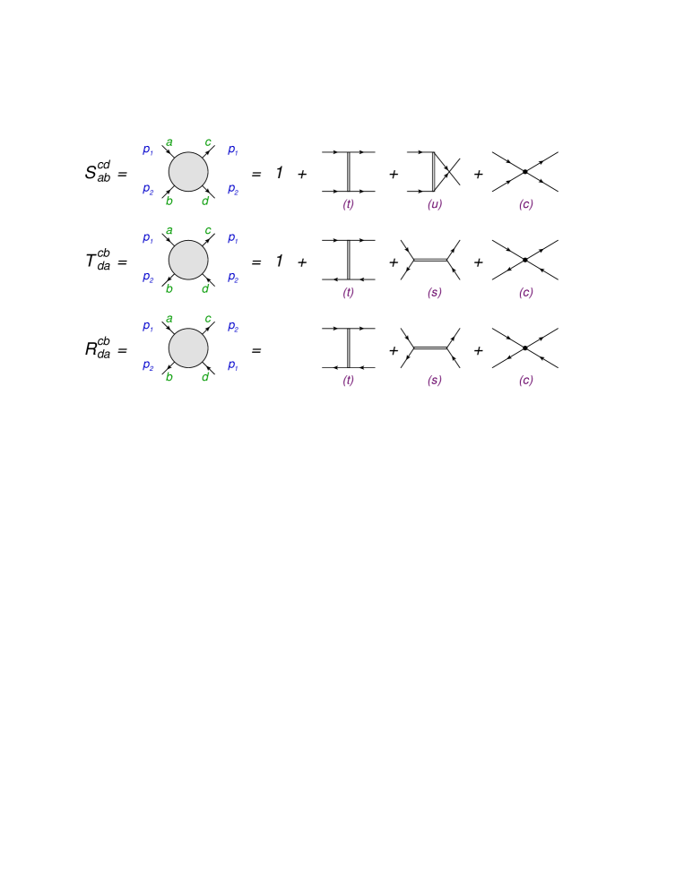
Figure 2: The scattering ($XX\rightarrow XX$), transmission ($X\bar{X}\rightarrow X\bar{X}$) and reflection ($X\bar{X}\rightarrow\bar{X}X$) amplitudes. At tree level, they are given by the sum of the contact interaction diagram (c) and the exchange graphs with the heavy mode $Z$ in the (s), (t), and (u) channels.

4.1 Worldsheet calculation

At tree level,

$$\mathbbm{S}_{ab}^{cd} = \delta_{a}^{c}\delta_{b}^{d}+\frac{2i}{\sqrt{2\lambda}}\,S_{ab}^{cd}+\ldots$$

$$\mathbbm{T}_{da}^{cb} = \delta_{a}^{c}\delta_{d}^{b}+\frac{2i}{\sqrt{2\lambda}}\,T_{da}^{cb}+\ldots$$

$$\mathbbm{R}_{da}^{cb} = \frac{2i}{\sqrt{2\lambda}}\,R_{da}^{cb}+\ldots.$$ (4.1)

The diagrams that contribute to $S_{ab}^{cd}$, $T_{da}^{cb}$ and $R_{da}^{cb}$ are shown in fig. 2. It is straightforward to compute these diagrams from the vertices in the gauge-fixed Lagrangian (2.16), (2.18), (2.20). In order to get the S-matrix elements one needs to take into account the Jacobian from the momentum-conservation delta-function:

$$\delta^{(2)}\left(p_{1}^{\mu}+p_{2}^{\mu}-k_{1}^{\mu}-k_{2}^{\mu}\right)=\frac{\varepsilon_{1}\varepsilon_{2}}{\varepsilon_{1}p_{2}-\varepsilon_{2}p_{1}}\left[\delta(p_{1}-k_{1})\delta(p_{2}-k_{2})-\delta(p_{1}-k_{2})\delta(p_{2}-k_{1})\right],$$ (4.2)

and the external leg factor $1/(4\varepsilon_{1}\varepsilon_{2})$. Collecting various pieces together, we get:

$$S_{ab}^{cd} = \frac{1}{4}\,\,\frac{1}{\varepsilon_{1}p_{2}-\varepsilon_{2}p_{1}}\left\{\left[\frac{1}{2}\left((p_{1}+p_{2})^{2}-2\varepsilon_{1}\varepsilon_{2}+4(1-2a)(\varepsilon_{1}p_{2}-\varepsilon_{2}p_{1})^{2}\right)_{(c)}+\varepsilon_{1}\varepsilon_{2}\,{}_{(t)}\right]\right.$$ (4.3)

$$\times\left.\delta_{a}^{c}\delta_{b}^{d}+\left[\frac{1}{8}\left(12p_{1}p_{2}-4\varepsilon_{1}\varepsilon_{2}-1\right)_{(c)}+\frac{1}{8}\left(4p_{1}p_{2}+4\varepsilon_{1}\varepsilon_{2}+1\right)_{(u)}\right]\delta_{a}^{d}\delta_{b}^{c}\right\}$$

$$T_{da}^{cb} = \frac{1}{4}\,\,\frac{1}{\varepsilon_{1}p_{2}-\varepsilon_{2}p_{1}}\left\{\left[\frac{1}{2}\left((p_{1}-p_{2})^{2}+2\varepsilon_{1}\varepsilon_{2}+4(1-2a)(\varepsilon_{1}p_{2}-\varepsilon_{2}p_{1})\right)_{(c)}-\varepsilon_{1}\varepsilon_{2}\,{}_{(t)}\right]\right.$$ (4.4)

$$\times\left.\delta_{a}^{c}\delta_{d}^{b}+\left[\frac{1}{8}\left(4\varepsilon_{1}\varepsilon_{2}-12p_{1}p_{2}-1\right)_{(c)}-\frac{1}{8}\left(4\varepsilon_{1}\varepsilon_{2}+4p_{1}p_{2}-1\right)_{(s)}\right]\delta_{a}^{b}\delta_{d}^{c}\right\}$$

$$R_{da}^{cb} = \frac{1}{4}\,\,\frac{1}{\varepsilon_{1}p_{2}-\varepsilon_{2}p_{1}}\left\{\left[\frac{1}{8}\left(4\varepsilon_{1}\varepsilon_{2}+p_{1}p_{2}+1\right)_{(c)}-\frac{1}{8}\left(4\varepsilon_{1}\varepsilon_{2}+p_{1}p_{2}+1\right)_{(t)}\right]\delta_{a}^{c}\delta_{d}^{b}\right.$$ (4.5)

$$\left.+\left[\frac{1}{8}\left(-4\varepsilon_{1}\varepsilon_{2}-p_{1}p_{2}+1\right)_{(c)}+\frac{1}{8}\left(4\varepsilon_{1}\varepsilon_{2}+p_{1}p_{2}-1\right)_{(s)}\right]\delta_{a}^{b}\delta_{d}^{c}\right\},$$

The contribution from the exchange diagrams is structurally similar to that of the contact interaction, and in fact the two contributions tend to cancel. In the case of the reflection amplitude the cancelation is complete:

$$S_{ab}^{cd} = \left[\frac{1}{8}\,\,\frac{(p_{1}+p_{2})^{2}}{\varepsilon_{1}p_{2}-\varepsilon_{2}p_{1}}+\frac{1}{2}\left(1-2a\right)\left(\varepsilon_{1}p_{2}-\varepsilon_{2}p_{1}\right)\right]\delta_{a}^{c}\delta_{b}^{d}+\frac{1}{2}\,\,\frac{p_{1}p_{2}}{\varepsilon_{1}p_{2}-\varepsilon_{2}p_{1}}\,\delta_{a}^{d}\delta_{b}^{c}$$ (4.6)

$$T_{da}^{cb} = \left[\frac{1}{8}\,\,\frac{(p_{1}-p_{2})^{2}}{\varepsilon_{1}p_{2}-\varepsilon_{2}p_{1}}+\frac{1}{2}\left(1-2a\right)\left(\varepsilon_{1}p_{2}-\varepsilon_{2}p_{1}\right)\right]\delta_{a}^{c}\delta_{d}^{b}-\frac{1}{2}\,\,\frac{p_{1}p_{2}}{\varepsilon_{1}p_{2}-\varepsilon_{2}p_{1}}\,\delta_{a}^{b}\delta_{d}^{c}$$ (4.7)

$$R_{da}^{cb} = 0.$$ (4.8)

The tree-level worldsheet S-matrix is indeed reflectionless, in accord with the conjectured absence of reflection in the exact soliton-antisoliton scattering [1]. Let us check that the transmission and scattering amplitudes also agree with the S-matrix proposed in [1].

4.2 Comparison to the exact result

The exact S-matrix is expressed in terms of the kinematic variables

$$x^{\pm}=\frac{1+\sqrt{1+16h^{2}(\lambda)\sin^{2}\frac{p}{\sqrt{2\lambda}}}}{4h(\lambda)\sin\frac{p}{\sqrt{2\lambda}}}\,\,{\rm e}\,^{\pm\frac{ip}{\sqrt{2\lambda}}},$$ (4.9)

which at strong coupling become

$$x^{\pm}\simeq\frac{1+2\varepsilon}{2p}\left(1\pm\frac{ip}{\sqrt{2\lambda}}\right).$$ (4.10)

The exact S-matrix of $AdS_{4}/CFT_{3}$ is the Beisert’s $PSU(2|2)$ S-matrix [30, 31] with an appropriate dressing phase. The $X^{a}X^{b}\rightarrow X^{c}X^{d}$ amplitude coincides with the S-matrix element for the scalar states of the $(2|2)$ multiplet:

$$\mathbb{S}_{ab}^{cd}=\,{\rm e}\,^{i\theta}\,\frac{1-\frac{1}{x_{1}^{+}x_{2}^{-}}}{1-\frac{1}{x_{1}^{+}x_{2}^{+}}}\,\,\frac{x_{1}^{-}-x_{2}^{-}}{x_{1}^{-}-x_{2}^{+}}\,\delta_{a}^{c}\delta_{b}^{d}+\,{\rm e}\,^{i\theta}\left(\frac{1-\frac{1}{x_{1}^{+}x_{2}^{-}}}{1-\frac{1}{x_{1}^{-}x_{2}^{+}}}\,\,\frac{x_{1}^{+}-x_{2}^{-}}{x_{1}^{-}-x_{2}^{+}}-\frac{1-\frac{1}{x_{1}^{+}x_{2}^{-}}}{1-\frac{1}{x_{1}^{+}x_{2}^{+}}}\,\,\frac{x_{1}^{-}-x_{2}^{-}}{x_{1}^{-}-x_{2}^{+}}\right)\delta_{a}^{d}\delta_{b}^{c},$$ (4.11)

The dressing phase $\theta$ is mildly gauge-dependent [47], and has the following general form:

$$\theta=\frac{1}{\sqrt{2\lambda}}\left[p_{2}-p_{1}-2a(\varepsilon_{1}p_{2}-\varepsilon_{2}p_{1})\right]-\frac{\sqrt{2\lambda}}{2}\sum_{r,s=\pm}rs\chi(x_{1}^{r},x_{2}^{s}).$$ (4.12)

where [48]

$$\chi(x,y)=(x-y)\left[\frac{1}{xy}+\left(1-\frac{1}{xy}\right)\ln\left(1-\frac{1}{xy}\right)\right]+O\left(\frac{1}{\sqrt{2\lambda}}\right).$$ (4.13)

Higher orders in the dressing phase are known exactly [33], and in fact non-perturbatively in $\lambda$ [32, 49], but we will only need the leading term explicitly shown in (4.13).

Expanding (4.11) in $1/\sqrt{2\lambda}$, we get:

$$\mathbb{S}_{ab}^{cd}\simeq\left\{1+\frac{i}{\sqrt{2\lambda}}\left[\frac{1}{4}\,\,\frac{(p_{1}+p_{2})^{2}}{\varepsilon_{1}p_{2}-\varepsilon_{2}p_{1}}+\left(1-2a\right)\left(\varepsilon_{1}p_{2}-\varepsilon_{2}p_{1}\right)\right]\right\}\delta_{a}^{c}\delta_{b}^{d}+\frac{i}{\sqrt{2\lambda}}\,\,\frac{p_{1}p_{2}}{\varepsilon_{1}p_{2}-\varepsilon_{2}p_{1}}\,\delta_{a}^{d}\delta_{b}^{c},$$ (4.14)

which agrees precisely with the explicit worldsheet calculation (4.1), (4.6).

To compare the $X^{a}\bar{X}_{b}\rightarrow X^{c}\bar{X}_{d}$ transmission amplitude with the exact S-matrix of Ahn and Nepomechie [1], we should take into account that in [1] the S-matrix is expressed in terms of the fields with the upper $su(2)$ indices: $B^{a}=\varepsilon^{ab}\bar{X}_{b}$. The transmission amplitude is again given by the Beisert’s $PSU(2|2)$ S-matrix, with an addition dressing factor. The transmission matrix $\mathbb{T}_{da}^{cb}$ defined in fig. 2 is then proportional to the $XX\rightarrow XX$ scattering matrix:

$$\mathbb{T}_{da}^{cb}=S_{0}\varepsilon^{bf}\varepsilon_{de}\mathbb{S}_{af}^{ce},$$ (4.15)

where [1]

$$S_{0}=\frac{1-\frac{1}{x_{1}^{-}x_{2}^{+}}}{1-\frac{1}{x_{1}^{+}x_{2}^{-}}}\,\,\frac{x_{1}^{-}-x_{2}^{+}}{x_{1}^{+}-x_{2}^{-}}\,.$$ (4.16)

If we write

$$\mathbb{S}_{ab}^{cd}=A\delta_{a}^{c}\delta_{b}^{d}+B\delta_{a}^{d}\delta_{b}^{c},$$ (4.17)

then

$$\mathbb{T}_{da}^{cb}=S_{0}\left(A+B\right)\delta_{a}^{c}\delta_{d}^{b}-S_{0}B\delta_{a}^{b}\delta_{d}^{c}.$$ (4.18)

The additional factor $S_{0}$ expands at strong coupling as

$$S_{0}\simeq 1-\frac{i}{\sqrt{2\lambda}}\,\,\frac{2p_{1}p_{2}}{\varepsilon_{1}p_{2}-\varepsilon_{2}p_{1}}\,,$$ (4.19)

and from (4.18), (4.14) we find:

$$\mathbb{T}_{da}^{cb}\simeq\left\{1+\frac{i}{\sqrt{2\lambda}}\left[\frac{1}{4}\,\frac{(p_{1}-p_{2})^{2}}{\varepsilon_{1}p_{2}-\varepsilon_{2}p_{1}}+\left(1-2a\right)\left(\varepsilon_{1}p_{2}-\varepsilon_{2}p_{1}\right)\right]\right\}\delta_{a}^{c}\delta_{d}^{b}-\frac{i}{\sqrt{2\lambda}}\,\frac{p_{1}p_{2}}{\varepsilon_{1}p_{2}-\varepsilon_{2}p_{1}}\,\delta_{a}^{b}\delta_{d}^{c},$$ (4.20)

again in the precise agreement with the direct worldsheet calculation.

5 Conclusions

In this paper we studied the fate of the heavy BMN modes in type IIA string theory on $AdS_{4}\times CP^{3}$. We argued that once the quantum corrections are taken into account the heavy modes mix with the two-particle continuum of the light modes and disappear from the spectrum. This picture is confirmed by an explicit one-loop calculation in the worldsheet sigma-model and is consistent with the Bethe ansatz solution of the $AdS_{4}/CFT_{3}$ system, where heavy modes were interpreted as stacks of Bethe roots. The true physical excitations on the string worldsheet are the $4+4$ light modes. It is interesting that all the bosonic light modes are fluctuations in the $CP^{3}$ directions. The transverse modes in $AdS_{4}$ disappear by mixing with the two-fermion states. This is in a qualitative agreement with the spin-chain picture of the spectrum in the dual $\mathcal{N}=6$ Chern-Simons theory. The AdS directions are dual to the covariant derivatives in the field-theory operators. In the Chern-Simons spin chain, the derivative operators mix with fermions: $\Phi D_{\mu}\Phi\leftrightarrow\bar{\Psi}_{\alpha}\sigma_{\mu}^{\hphantom{\mu}\alpha\beta}\Psi_{\beta}$, and do not form a closed sector [7] .

Despite that the heavy modes disappear from the spectrum, the corresponding fields appear as intermediate states in the perturbative worldsheet S-matrix. In fact, the exchange of the heavy modes is crucially important for cancelation of the reflection amplitude in the particle-antiparticle scattering. We also checked that the scattering and transmission amplitudes computed in the light-cone sigma-model agree with the large-$\lambda$ expansion of the exact S-matrix proposed in [1].

Acknowledgments

I would like to thank C. Ahn, G. Arutyunov, S. Frolov, S. Hirano, D. Hofman, J. Maldacena, J. Minahan, S.-J. Rey, P. Vieira and especially T. Harmark and M. Orselli for interesting discussions. I also thank the organizers of the the 29th winter school ”Geometry and Physics” in Srni and of the workshop ”Gauge Fields, Cosmology and Mathematical String Theory” in Banff for hospitality during the course of this work. This work was supported in part by the Swedish Research Council under the contract 621-2007-4177, in part by the RFFI grant 09-02-00253, and in part by the grant for support of scientific schools NSH-3036.2008.2.

Appendix A The $osp(6|4)$ superalgebra

The (anti)commutation relations of $osp(6|4)$ in the basis (2) are

$$[R^{a}_{b},R^{c}_{d}]=\delta^{a}_{d}R^{c}_{b}-\delta^{c}_{b}R^{a}_{d},\qquad[R^{a}_{b},R^{c}]=\delta^{a}_{b}R^{c}-\delta^{c}_{b}R^{a},\qquad[R^{a}_{b},R_{c}]=-\delta^{a}_{b}R_{c}+\delta^{a}_{c}R_{b},$$

$$[R^{a},R_{b}]=\delta^{a}_{b}\left(R^{c}_{c}-R\right)-R^{a}_{b},\qquad[R,R^{a}]=-R^{a},\qquad[R,R_{a}]=R_{a},$$

$$[T_{i},T_{j}]=\varepsilon_{ijk}T_{k},\qquad[T_{i},K_{j}]=\varepsilon_{ijk}K_{k},\qquad[K_{i},K_{j}]=-\varepsilon_{ijk}T_{k},$$

$$[R^{a}_{b},B^{c}]=-\delta^{c}_{b}B^{a},\qquad[R^{a}_{b},B_{c}]=\delta^{a}_{c}B_{b},\qquad[R^{a},B_{b}]=\frac{1}{2}\,\delta^{a}_{b}\left(J+M\right),$$

$$[R_{a},B^{b}]=\frac{1}{2}\,\delta^{b}_{a}\left(J-M\right),\qquad[R,B^{a}]=-B^{a},\qquad[R,B_{a}]=B_{a},$$

$$[J,R^{a}_{b}]=-\delta^{a}_{b}M,\qquad[J,R^{a}]=-B^{a},\qquad[J,R_{a}]=-B_{a},$$

$$[M,R^{a}_{b}]=-\delta^{a}_{b}J,\qquad[M,R^{a}]=B^{a},\qquad[M,R_{a}]=-B_{a},$$

$$[T_{i},L_{j}]=\varepsilon_{ijk}L_{k},\qquad[K_{i},L_{j}]=-\delta_{ij}D,\qquad[D,K_{i}]=L_{i},$$

$$[B^{a},B_{b}]=\delta^{a}_{b}R+R^{a}_{b},\qquad[J,B^{a}]=-R^{a},\qquad[J,B_{a}]=-R_{a},\qquad[J,M]=-2R^{a}_{a},$$

$$[M,B^{a}]=-R^{a},\qquad[M,B_{a}]=R_{a},\qquad[D,L_{i}]=-K_{i},\qquad[L_{i},L_{j}]=-\varepsilon_{ijk}T_{k},$$

$$[R^{a}_{b},Q^{c}_{\alpha}]=-\delta^{c}_{b}Q^{a}_{\alpha},\qquad[R^{a}_{b},\bar{Q}_{c\alpha}]=\delta^{a}_{c}\bar{Q}_{b\alpha},\qquad[R^{a},Q^{b}_{\alpha}]=-\varepsilon^{ab}Q_{\alpha},$$

$$[R^{a},\bar{Q}_{\alpha}]=\varepsilon^{ab}\bar{Q}_{b\alpha},\qquad[R_{a},\bar{Q}_{b\alpha}]=\varepsilon_{ab}\bar{Q}_{\alpha},\qquad[R_{a},Q_{\alpha}]=-\varepsilon_{ab}Q^{b}_{\alpha},$$

$$[R,Q_{\alpha}]=-Q_{\alpha},\qquad[R,\bar{Q}_{\alpha}]=\bar{Q}_{\alpha},\qquad[K_{i},Q^{a}_{\alpha}]=\frac{1}{2}\,\sigma_{i\alpha}^{\hphantom{i\alpha}\beta}Q^{a}_{\beta},$$

$$[K_{i},Q_{\alpha}]=\frac{1}{2}\,\sigma_{i\alpha}^{\hphantom{i\alpha}\beta}Q_{\beta},\qquad[K_{i},\bar{Q}_{a\alpha}]=-\frac{1}{2}\,\sigma_{i\alpha}^{\hphantom{i\alpha}\beta}\bar{Q}_{a\beta},\qquad[K_{i},\bar{Q}_{\alpha}]=-\frac{1}{2}\,\sigma_{i\alpha}^{\hphantom{i\alpha}\beta}\bar{Q}_{\beta},$$

$$[T_{i},Q^{a}_{\alpha}]=\frac{i}{2}\,\sigma_{i\alpha}^{\hphantom{i\alpha}\beta}Q^{a}_{\beta},\qquad[T_{i},Q_{\alpha}]=\frac{i}{2}\,\sigma_{i\alpha}^{\hphantom{i\alpha}\beta}Q_{\beta},$$

$$[T_{i},\bar{Q}_{a\alpha}]=\frac{i}{2}\,\sigma_{i\alpha}^{\hphantom{i\alpha}\beta}\bar{Q}_{a\beta},\qquad[T_{i},\bar{Q}_{\alpha}]=\frac{i}{2}\,\sigma_{i\alpha}^{\hphantom{i\alpha}\beta}\bar{Q}_{\beta},$$

$$[R^{a}_{b},S_{c\alpha}]=\delta^{a}_{c}S_{b\alpha},\qquad[R^{a}_{b},\bar{S}^{c}_{\alpha}]=-\delta^{c}_{b}\bar{S}^{a}_{\alpha},\qquad[R^{a},\bar{S}^{b}_{\alpha}]=-\varepsilon^{ab}\bar{S}_{\alpha},$$

$$[R^{a},S_{\alpha}]=\varepsilon^{ab}S_{b\alpha},\qquad[R_{a},S_{b\alpha}]=\varepsilon_{ab}S_{\alpha},\qquad[R_{a},\bar{S}_{\alpha}]=-\varepsilon_{ab}\bar{S}^{b}_{\alpha},$$

$$[R,S_{\alpha}]=S_{\alpha},\qquad[R,\bar{S}_{\alpha}]=-\bar{S}_{\alpha},\qquad[K_{i},S_{a\alpha}]=\frac{1}{2}\,\sigma_{i\alpha}^{\hphantom{i\alpha}\beta}S_{a\beta},$$

$$[K_{i},S_{\alpha}]=\frac{1}{2}\,\sigma_{i\alpha}^{\hphantom{i\alpha}\beta}S_{\beta},\qquad[K_{i},\bar{S}^{a}_{\alpha}]=-\frac{1}{2}\,\sigma_{i\alpha}^{\hphantom{i\alpha}\beta}\bar{S}^{a}_{\beta},\qquad[K_{i},\bar{S}_{\alpha}]=-\frac{1}{2}\,\sigma_{i\alpha}^{\hphantom{i\alpha}\beta}\bar{S}_{\beta},$$

$$[T_{i},S_{a\alpha}]=\frac{i}{2}\,\sigma_{i\alpha}^{\hphantom{i\alpha}\beta}S_{a\beta},\qquad[T_{i},S_{\alpha}]=\frac{i}{2}\,\sigma_{i\alpha}^{\hphantom{i\alpha}\beta}S_{\beta},$$

$$[T_{i},\bar{S}^{a}_{\alpha}]=\frac{i}{2}\,\sigma_{i\alpha}^{\hphantom{i\alpha}\beta}\bar{S}^{a}_{\beta},\qquad[T_{i},\bar{S}_{\alpha}]=\frac{i}{2}\,\sigma_{i\alpha}^{\hphantom{i\alpha}\beta}\bar{S}_{\beta},$$

$$[B^{a},\bar{Q}_{b\alpha}]=\delta^{a}_{b}\bar{S}_{\alpha},\qquad[B^{a},\bar{Q}_{\alpha}]=-\bar{S}^{a}_{\alpha},\qquad[B_{a},Q^{b}_{\alpha}]=\delta^{b}_{a}S_{\alpha},\qquad[B_{a},Q_{\alpha}]=-S_{a\alpha},$$

$$[J,Q^{a}_{\alpha}]=\varepsilon^{ab}S_{b\alpha},\qquad[J,\bar{Q}_{a\alpha}]=-\varepsilon_{ab}\bar{S}^{b}_{\alpha},\qquad[M,Q^{a}_{\alpha}]=\varepsilon^{ab}S_{b\alpha},$$

$$[M,\bar{Q}_{a\alpha}]=\varepsilon_{ab}\bar{S}^{b}_{\alpha},\qquad[L_{i},Q^{a}_{\alpha}]=\frac{1}{2}\,\sigma_{i\alpha}^{\hphantom{i\alpha}\beta}\bar{S}^{a}_{\beta},\qquad[L_{i},Q_{\alpha}]=\frac{1}{2}\,\sigma_{i\alpha}^{\hphantom{i\alpha}\beta}\bar{S}_{\beta},$$

$$[L_{i},\bar{Q}_{a\alpha}]=\frac{1}{2}\,\sigma_{i\alpha}^{\hphantom{i\alpha}\beta}S_{a\beta},\qquad[L_{i},\bar{Q}_{\alpha}]=\frac{1}{2}\,\sigma_{i\alpha}^{\hphantom{i\alpha}\beta}S_{\beta},\qquad[D,Q^{a}_{\alpha}]=\frac{1}{2}\,\bar{S}^{a}_{\alpha},$$

$$[D,Q_{\alpha}]=\frac{1}{2}\,\bar{S}_{\alpha},\qquad[D,\bar{Q}_{a\alpha}]=-\frac{1}{2}\,S_{a\alpha},\qquad[D,\bar{Q}_{\alpha}]=-\frac{1}{2}\,S_{\alpha},$$

$$[B^{a},S_{b\alpha}]=\delta^{a}_{b}Q_{\alpha},\qquad[B^{a},S_{\alpha}]=-Q^{a}_{\alpha},\qquad[B_{a}\bar{S}^{b}_{\alpha}]=\delta^{b}_{a}\bar{Q}_{\alpha},\qquad[B_{a},\bar{S}_{\alpha}]=-\bar{Q}_{a\alpha},$$

$$[J,\bar{S}^{a}_{\alpha}]=\varepsilon^{ab}\bar{Q}_{b\alpha},\qquad[J,S_{a\alpha}]=-\varepsilon_{ab}Q^{b}_{\alpha},\qquad[M,\bar{S}^{a}_{\alpha}]=\varepsilon^{ab}\bar{Q}_{b\alpha},$$

$$[M,S_{a\alpha}]=\varepsilon_{ab}Q^{b}_{\alpha},\qquad[L_{i},S_{a\alpha}]=\frac{1}{2}\,\sigma_{i\alpha}^{\hphantom{i\alpha}\beta}\bar{Q}_{a\beta},\qquad[L_{i},S_{\alpha}]=\frac{1}{2}\,\sigma_{i\alpha}^{\hphantom{i\alpha}\beta}\bar{Q}_{\beta},$$

$$[L_{i},\bar{S}^{a}_{\alpha}]=\frac{1}{2}\,\sigma_{i\alpha}^{\hphantom{i\alpha}\beta}Q^{a}_{\beta},\qquad[L_{i},\bar{S}_{\alpha}]=\frac{1}{2}\,\sigma_{i\alpha}^{\hphantom{i\alpha}\beta}Q_{\beta},\qquad[D,S_{a\alpha}]=\frac{1}{2}\,\bar{Q}_{a\alpha},$$

$$[D,S_{\alpha}]=\frac{1}{2}\,\bar{Q}_{\alpha},\qquad[D,\bar{S}^{a}_{\alpha}]=-\frac{1}{2}\,Q^{a}_{\alpha},\qquad[D,\bar{S}_{\alpha}]=-\frac{1}{2}\,Q_{\alpha},$$

$$\{Q^{a}_{\alpha},Q^{b}_{\beta}\}=-\frac{i}{2}\,\varepsilon_{\alpha\beta}\varepsilon^{ab}\left(J-M\right),\qquad\{Q^{a}_{\alpha},Q_{\beta}\}=i\varepsilon_{\alpha\beta}B^{a},$$

$$\{Q^{a}_{\alpha},\bar{Q}_{b\beta}\}=-i\delta^{a}_{b}\left[\varepsilon_{\alpha\beta}D-\left(\sigma_{i}\varepsilon\right)_{\alpha\beta}L_{i}\right],\qquad\{Q_{\alpha},\bar{Q}_{\beta}\}=-i\left[\varepsilon_{\alpha\beta}D-\left(\sigma_{i}\varepsilon\right)_{\alpha\beta}L_{i}\right],$$

$$\{\bar{Q}_{a\alpha},\bar{Q}_{b\beta}\}=\frac{i}{2}\,\varepsilon_{\alpha\beta}\varepsilon_{ab}\left(J+M\right),\qquad\{\bar{Q}_{a\alpha},\bar{Q}_{\beta}\}=i\varepsilon_{\alpha\beta}B_{a},$$

$$\{S_{a\alpha},S_{b\beta}\}=\frac{i}{2}\,\varepsilon_{\alpha\beta}\varepsilon_{ab}\left(J+M\right),\qquad\{S_{a\alpha},S_{\beta}\}=i\varepsilon_{\alpha\beta}B_{a},$$

$$\{S_{a\alpha},\bar{S}^{b}_{\beta}\}=-i\delta^{b}_{a}\left[\varepsilon_{\alpha\beta}D-\left(\sigma_{i}\varepsilon\right)_{\alpha\beta}L_{i}\right],\qquad\{S_{\alpha},\bar{S}_{\beta}\}=-i\left[\varepsilon_{\alpha\beta}D-\left(\sigma_{i}\varepsilon\right)_{\alpha\beta}L_{i}\right],$$

$$\{\bar{S}^{a}_{\alpha},\bar{S}^{b}_{\beta}\}=-\frac{i}{2}\,\varepsilon_{\alpha\beta}\varepsilon^{ab}\left(J-M\right),\qquad\{\bar{S}^{a}_{\alpha},\bar{S}_{\beta}\}=i\varepsilon_{\alpha\beta}B^{a},$$

$$\{Q^{a}_{\alpha},S_{b\beta}\}=i\delta^{a}_{b}\left(\sigma_{i}\varepsilon\right)_{\alpha\beta}\left(K_{i}-iT_{i}\right)+i\varepsilon_{\alpha\beta}R^{a}_{b},\qquad\{Q^{a}_{\alpha},S_{\beta}\}=-i\varepsilon_{\alpha\beta}\varepsilon^{ab}R_{b},$$

$$\{Q_{\alpha},S_{a\beta}\}=-i\varepsilon_{\alpha\beta}\varepsilon_{ab}R^{b},\qquad\{Q_{\alpha},S_{\beta}\}=i\left(\sigma_{i}\varepsilon\right)_{\alpha\beta}\left(K_{i}-iT_{i}\right)+i\varepsilon_{\alpha\beta}R,$$

$$\{\bar{Q}_{a\alpha},\bar{S}^{b}_{\beta}\}=-i\delta^{b}_{a}\left(\sigma_{i}\varepsilon\right)_{\alpha\beta}\left(K_{i}+iT_{i}\right)-i\varepsilon_{\alpha\beta}R^{b}_{a},\qquad\{\bar{Q}_{a\alpha},\bar{S}_{\beta}\}=i\varepsilon_{\alpha\beta}\varepsilon_{ab}R^{b},$$

$$\{\bar{Q}_{\alpha},\bar{S}^{a}_{\beta}\}=i\varepsilon_{\alpha\beta}\varepsilon^{ab}R_{b},\qquad\{\bar{Q}_{\alpha},\bar{S}_{\beta}\}=-i\left(\sigma_{i}\varepsilon\right)_{\alpha\beta}\left(K_{i}+iT_{i}\right)-i\varepsilon_{\alpha\beta}R,$$ (A.1)

where $\sigma_{i\alpha}^{\hphantom{i\alpha}\beta}$ are Pauli matrices.

The non-zero components of the invariant metric are

$$\mathop{\mathrm{Str}}R^{a}_{b}R^{c}_{d}=-\delta^{a}_{d}\delta^{c}_{b},\qquad\mathop{\mathrm{Str}}R^{a}R_{b}=-\delta^{a}_{b},\qquad\mathop{\mathrm{Str}}R^{2}=-1,\qquad\mathop{\mathrm{Str}}B^{a}B_{b}=\delta^{a}_{b}$$

$$\mathop{\mathrm{Str}}J^{2}=-2,\qquad\mathop{\mathrm{Str}}M^{2}=2,\qquad\mathop{\mathrm{Str}}D^{2}=-\frac{1}{2}\,,\qquad\mathop{\mathrm{Str}}L_{i}L_{j}=\frac{1}{2}\,\delta_{ij},$$

$$\mathop{\mathrm{Str}}K_{i}K_{j}=\frac{1}{2}\,\delta_{ij},\qquad\mathop{\mathrm{Str}}T_{i}T_{j}=-\frac{1}{2}\,\delta_{ij},\qquad\mathop{\mathrm{Str}}Q^{a}_{\alpha}S_{b\beta}=i\varepsilon_{\alpha\beta}\delta^{a}_{b},$$

$$\mathop{\mathrm{Str}}Q_{\alpha}S_{\beta}=i\varepsilon_{\alpha\beta},\qquad\mathop{\mathrm{Str}}\bar{Q}_{a\alpha}\bar{S}^{b}_{\beta}=i\varepsilon_{\alpha\beta}\delta^{b}_{a},\qquad\mathop{\mathrm{Str}}\bar{Q}_{\alpha}\bar{S}_{\beta}=i\varepsilon_{\alpha\beta}.$$ (A.2)

Appendix B Light-cone gauge

In this appendix we consider the light-cone gauge fixing for the bosonic string in the background

$$ds^{2}=-G_{tt}dt^{2}+G_{\varphi\varphi}d\varphi^{2}+2G_{\varphi i}d\varphi dx^{i}+G_{ij}dx^{i}dx^{j},$$ (B.1)

where $G_{tt}$, $G_{\varphi\varphi}$, $G_{\varphi i}$ and $G_{ij}$ are functions of $x^{i}$. This is a slight generalization over [50, 47] where the case of $G_{\varphi i}=0$ has been considered.

The light-cone gauge fixing can be done in three steps [51]: one can T-dualize in the $\varphi$ direction, integrate out the worldsheet metric and then fix the gauge in the resulting Nambu-Goto action. This yields a non-polynomial Lagrangian, which can be further expanded in the transverse fluctuations. T-duality is equivalent to gauging the isometry

$$\varphi\rightarrow\varphi-(1-a)\xi,\qquad t\rightarrow t+a\xi$$ (B.2)

of the metric (B.1), and then imposing the flatness condition on the gauge connection. Here $0\leqslant a\leqslant 1/2$ is a gauge parameter that interpolated between the temporal ($a=0$) and light-cone ($a=1/2$) gauges [46]. The worldsheet Lagrangian becomes

$$\mathcal{L} = -\frac{G_{tt}}{2}\left(\partial_{\mu}t+aA_{\mu}\right)^{2}+\frac{G_{\varphi\varphi}}{2}\left[\partial_{\mu}\varphi-\left(1-a\right)A_{\mu}\right]^{2}$$ (B.3)

$$+G_{\varphi i}\left[\partial_{\mu}\varphi-\left(1-a\right)A_{\mu}\right]\partial^{\mu}X^{i}+\frac{G_{ij}}{2}\,\partial_{\mu}X^{i}\partial^{\mu}X^{j}+\frac{1}{\sqrt{-h}}\,\tilde{\varphi}\varepsilon^{\mu\nu}\partial_{\mu}A_{\nu},$$

where $\tilde{\varphi}$ is a Lagrange multiplier that imposes the flatness condition on $A_{\mu}$. The equations of motion for $A_{\mu}$ imply that

$$\varepsilon^{\mu\nu}\partial_{\nu}\tilde{\varphi}=\frac{J^{\mu}}{T}\,,$$ (B.4)

where $J^{\mu}$ is the Neother current associated with the isometry (B.2) and $T$ is the string tension ($T=\sqrt{2\lambda}/2$ in $AdS_{4}\times CP^{3}$). Setting $\mu=0$ and integrating along the fixed-time section of the string worldsheet, we find:

$$\tilde{\varphi}(x^{0},x^{1}+L)-\tilde{\varphi}(x^{0},x^{1})=\int_{-L/2}^{L/2}dx^{1}\,\partial_{1}\tilde{\varphi}=\mathcal{J}_{+}\equiv\frac{J_{+}}{T}\,,$$ (B.5)

where $J_{+}$ is the corresponding Neother charge ($J_{+}=(1-a)J+aE$, where $J$ is the angular momentum of the string and $E$ is its energy), and $L$ is the internal length of the string that can be chosen arbitrarily due to the reparameterization invariance.

The T-dual Lagrangian arises after integrating out $A_{\mu}$ in (B.3):

$$\tilde{\mathcal{L}} = \frac{1}{2}\,\,\frac{1}{\left(1-a\right)^{2}G_{\varphi\varphi}-a^{2}G_{tt}}\left\{-G_{tt}G_{\varphi\varphi}\left(\partial_{\mu}X^{+}\right)^{2}+\left(\partial_{\mu}\tilde{\varphi}\right)^{2}-2aG_{tt}G_{\varphi i}\partial_{\mu}X^{+}\partial^{\mu}X^{i}\vphantom{\frac{a}{1-a}}\right.$$ (B.6)

$$\left.+\tilde{G}_{ij}\partial_{\mu}X^{i}\partial^{\mu}X^{j}-\frac{1}{\sqrt{-h}}\,\varepsilon^{\mu\nu}\partial_{\mu}\tilde{\varphi}\left[\frac{a}{1-a}G_{tt}\partial_{\nu}X^{+}+\left(1-a\right)G_{\varphi i}\partial_{\nu}X^{i}\right]\right\},$$

where

$$X^{+}=\left(1-a\right)t+a\varphi,$$ (B.7)

and the T-dual transverse metric is

$$\tilde{G}_{ij}=\left[\left(1-a\right)^{2}G_{\varphi\varphi}-a^{2}G_{tt}\right]G_{ij}-\left(1-a\right)^{2}G_{\varphi i}G_{\varphi j}.$$ (B.8)

The corresponding Nambu-Goto Lagrangian is

$$\mathcal{L}_{\rm NG} = -\frac{1}{\left(1-a\right)^{2}G_{\varphi\varphi}-a^{2}G_{tt}}\left\{\vphantom{\frac{aG_{tt}}{1-a}}\left[\vphantom{+\left(aG_{tt}G_{\varphi i}\partial_{1}X^{i}-\tilde{G}_{ij}\partial_{1}X^{i}\partial_{1}X^{j}\right)^{2}}\left(G_{tt}G_{\varphi\varphi}+2aG_{tt}G_{\varphi i}\partial_{0}X^{i}-\tilde{G}_{ij}\partial_{0}X^{i}\partial_{0}X^{j}\right)\right.\right.$$ (B.9)

$$\left.\left.\times\left(1+\tilde{G}_{ij}\partial_{1}X^{i}\partial_{1}X^{j}\right)+\left(aG_{tt}G_{\varphi i}\partial_{1}X^{i}-\tilde{G}_{ij}\partial_{0}X^{i}\partial_{1}X^{j}\right)^{2}\right]^{1/2}\right.$$

$$\left.-\frac{aG_{tt}}{1-a}-\left(1-a\right)G_{\varphi i}\partial_{0}X^{i}\right\}.$$

This is written in the gauge

$$X^{+}=\tau,\qquad\tilde{\varphi}=\sigma.$$ (B.10)

The consistency of this gauge with the boundary condition (B.5) requires that the length of the string is identified with the light-cone momentum in the units of the string tension:

$$L=\mathcal{J}_{+}.$$ (B.11)

Of course one can choose arbitrary $L$, but then the gauge condition should be replaced by $\tilde{\varphi}=\mathcal{J}_{+}\sigma/L$, and the factor $\mathcal{J}_{+}/L$ will appear in many places in the gauge fixed Lagrangian. The choice (B.11) has an advantage that all the coefficients in the Lagrangian are pure numbers. The only coupling constant is an overall factor of the string tension.

The Nambu-Goto action (B.9) can be readily expanded in the transverse fluctuations. If we assume that $G_{tt}=1+O(X^{2})$, $G_{\varphi\varphi}=1+O(X^{2})$ and $G_{\varphi i}=O(X^{3})$, then up to the quartic order:

$$\mathcal{L}_{\rm NG} = \frac{G_{ij}}{2}\,\partial_{\mu}X^{i}\partial^{\mu}X^{j}-\frac{G_{tt}}{2}+\frac{G_{\varphi\varphi}}{2}+G_{\varphi i}\partial_{0}X^{i}$$ (B.12)

$$+\frac{1}{4}\left(1-G_{tt}G_{\varphi\varphi}\right)G_{ij}\left(\partial_{0}X^{i}\partial_{0}X^{j}+\partial_{1}X^{i}\partial_{1}X^{j}\right)+\frac{1}{4}\left(G_{tt}-1\right)^{2}-\frac{1}{4}\left(G_{\varphi\varphi}-1\right)^{2}$$

$$-\frac{1-2a}{8}\left({G_{tt}}-{G_{\varphi\varphi}}\right)^{2}-\frac{1-2a}{8}\left(G_{ij}\partial_{\mu}X^{i}\partial^{\mu}X^{j}\right)^{2}$$

$$+\frac{1-2a}{4}\left(G_{ij}\partial_{\mu}X^{i}\partial_{\nu}X^{j}\right)^{2}+\ldots.$$

The first line is the naive Lagrangian obtained by setting $t=\tau=\varphi$ in the Polyakov action, the second line is an additional gauge-invariant interaction that arises at the quartic order, the last two lines are gauge-dependent and vanish in the pure light-cone gauge $a=1/2$.

References

• [1] C. Ahn and R. I. Nepomechie, “N=6 super Chern-Simons theory S-matrix and all-loop Bethe ansatz equations”, JHEP 0809, 010 (2008), 0807.1924.
• [2] O. Aharony, O. Bergman, D. L. Jafferis and J. Maldacena, “N=6 superconformal Chern-Simons-matter theories, M2-branes and their gravity duals”, JHEP 0810, 091 (2008), 0806.1218.
• [3] O. Aharony, O. Bergman and D. L. Jafferis, “Fractional M2-branes”, JHEP 0811, 043 (2008), 0807.4924.
• [4] G. Arutyunov and S. Frolov, “Superstrings on $AdS_{4}\times CP^{3}$ as a Coset Sigma-model”, JHEP 0809, 129 (2008), 0806.4940.
• [5] j. Stefanski, B., “Green-Schwarz action for Type IIA strings on $AdS_{4}\times CP^{3}$, Nucl. Phys. B808, 80 (2009), 0806.4948.
• [6] J. Gomis, D. Sorokin and L. Wulff, “The complete $AdS_{4}\times CP^{3}$ superspace for the type IIA superstring and D-branes”, JHEP 0903, 015 (2009), 0811.1566.
• [7] J. A. Minahan and K. Zarembo, “The Bethe ansatz for superconformal Chern-Simons”, JHEP 0809, 040 (2008), 0806.3951.
• [8] N. Gromov and P. Vieira, “The AdS4/CFT3 algebraic curve”, JHEP 0902, 040 (2009), 0807.0437.
• [9] N. Gromov and P. Vieira, “The all loop AdS4/CFT3 Bethe ansatz”, JHEP 0901, 016 (2009), 0807.0777.
• [10] N. Gromov, V. Kazakov and P. Vieira, “Integrability for the Full Spectrum of Planar AdS/CFT”, 0901.3753.
• [11] D. Gaiotto, S. Giombi and X. Yin, “Spin Chains in N=6 Superconformal Chern-Simons-Matter Theory”, JHEP 0904, 066 (2009), 0806.4589.
• [12] D. Bak and S.-J. Rey, “Integrable Spin Chain in Superconformal Chern-Simons Theory”, JHEP 0810, 053 (2008), 0807.2063.
• [13] D. Bak, D. Gang and S.-J. Rey, “Integrable Spin Chain of Superconformal U(M)xU(N) Chern- Simons Theory”, JHEP 0810, 038 (2008), 0808.0170.
• [14] B. I. Zwiebel, “Two-loop Integrability of Planar N=6 Superconformal Chern- Simons Theory”, 0901.0411.
• [15] J. A. Minahan, W. Schulgin and K. Zarembo, “Two loop integrability for Chern-Simons theories with N=6 supersymmetry”, JHEP 0903, 057 (2009), 0901.1142.
• [16] O. Bergman and S. Hirano, “Anomalous radius shift in AdS(4)/CFT(3)”, 0902.1743.
• [17] T. Nishioka and T. Takayanagi, “On Type IIA Penrose Limit and N=6 Chern-Simons Theories”, JHEP 0808, 001 (2008), 0806.3391.
• [18] G. Grignani, T. Harmark and M. Orselli, “The SU(2) x SU(2) sector in the string dual of N=6 superconformal Chern-Simons theory”, Nucl. Phys. B810, 115 (2009), 0806.4959.
• [19] G. Grignani, T. Harmark, M. Orselli and G. W. Semenoff, “Finite size Giant Magnons in the string dual of N=6 superconformal Chern-Simons theory”, JHEP 0812, 008 (2008), 0807.0205.
• [20] B.-H. Lee, K. L. Panigrahi and C. Park, “Spiky Strings on $AdS_{4}\times{\bf CP}^{3}$, JHEP 0811, 066 (2008), 0807.2559.
• [21] I. Shenderovich, “Giant magnons in $AdS_{4}/CFT_{3}$: dispersion, quantization and finite-size corrections”, 0807.2861.
• [22] C. Ahn, P. Bozhilov and R. C. Rashkov, “Neumann-Rosochatius integrable system for strings on $AdS_{4}\times CP^{3}$, JHEP 0809, 017 (2008), 0807.3134.
• [23] S. Ryang, “Giant Magnon and Spike Solutions with Two Spins in $AdS_{4}\times CP^{3}$, JHEP 0811, 084 (2008), 0809.5106.
• [24] D. Bombardelli and D. Fioravanti, “Finite-Size Corrections of the $\mathbb{CP}^{3}$ Giant Magnons: the Lúscher terms”, 0810.0704.
• [25] T. Lukowski and O. O. Sax, “Finite size giant magnons in the SU(2) x SU(2) sector of $AdS_{4}xCP^{3}$, JHEP 0812, 073 (2008), 0810.1246.
• [26] C. Ahn and P. Bozhilov, “Finite-size Effect of the Dyonic Giant Magnons in N=6 super Chern-Simons Theory”, 0810.2079.
• [27] M. C. Abbott and I. Aniceto, “Giant Magnons in $AdS_{4}\times CP^{3}$: Embeddings, Charges and a Hamiltonian”, 0811.2423.
• [28] C. Kalousios, M. Spradlin and A. Volovich, “Dyonic Giant Magnons on $CP^{3}$, 0902.3179.
• [29] R. Suzuki, “Giant Magnons on $CP^{3}$ by Dressing Method”, 0902.3368.
• [30] N. Beisert, “The su(2—2) dynamic S-matrix”, Adv. Theor. Math. Phys. 12, 945 (2008), hep-th/0511082.
• [31] N. Beisert, “The Analytic Bethe Ansatz for a Chain with Centrally Extended su(2—2) Symmetry”, J. Stat. Mech. 0701, P017 (2007), nlin/0610017.
• [32] N. Beisert, B. Eden and M. Staudacher, “Transcendentality and crossing”, J. Stat. Mech. 0701, P021 (2007), hep-th/0610251.
• [33] N. Beisert, R. Hernandez and E. Lopez, “A crossing-symmetric phase for $AdS_{5}\times S^{5}$ strings”, JHEP 0611, 070 (2006), hep-th/0609044.
• [34] C. Ahn and R. I. Nepomechie, “An alternative S-matrix for N=6 Chern-Simons theory ?”, JHEP 0903, 068 (2009), 0810.1915.
• [35] C. Ahn and R. I. Nepomechie, “Two-loop test of the N=6 Chern-Simons theory S-matrix”, JHEP 0903, 144 (2009), 0901.3334.
• [36] T. McLoughlin and R. Roiban, “Spinning strings at one-loop in $AdS_{4}\times P^{3}$, JHEP 0812, 101 (2008), 0807.3965.
• [37] L. F. Alday, G. Arutyunov and D. Bykov, “Semiclassical Quantization of Spinning Strings in $AdS_{4}\times CP^{3}$, JHEP 0811, 089 (2008), 0807.4400.
• [38] C. Krishnan, $AdS_{4}/CFT_{3}$ at One Loop”, JHEP 0809, 092 (2008), 0807.4561.
• [39] N. Gromov and V. Mikhaylov, “Comment on the Scaling Function in $AdS_{4}\times CP_{3}$, JHEP 0904, 083 (2009), 0807.4897.
• [40] T. McLoughlin, R. Roiban and A. A. Tseytlin, “Quantum spinning strings in $AdS_{4}\times CP^{3}$: testing the Bethe Ansatz proposal”, JHEP 0811, 069 (2008), 0809.4038.
• [41] N. Beisert, V. A. Kazakov, K. Sakai and K. Zarembo, “Complete spectrum of long operators in N = 4 SYM at one loop”, JHEP 0507, 030 (2005), hep-th/0503200.
• [42] N. Gromov and P. Vieira, “Complete 1-loop test of AdS/CFT”, JHEP 0804, 046 (2008), 0709.3487.
• [43] D. Astolfi, V. G. M. Puletti, G. Grignani, T. Harmark and M. Orselli, “Finite-size corrections in the SU(2) x SU(2) sector of type IIA string theory on $AdS_{4}xCP^{3}$, Nucl. Phys. B810, 150 (2009), 0807.1527.
• [44] P. Sundin, “The $AdS_{4}\times CP_{3}$ string and its Bethe equations in the near plane wave limit”, JHEP 0902, 046 (2009), 0811.2775.
• [45] D. V. Uvarov, $AdS_{4}\times CP^{3}$ superstring and D=3 N=6 superconformal symmetry”, 0811.2813.
• [46] G. Arutyunov, S. Frolov and M. Zamaklar, “Finite-size effects from giant magnons”, Nucl. Phys. B778, 1 (2007), hep-th/0606126.
• [47] G. Arutyunov and S. Frolov, “Foundations of the $AdS_{5}\times S^{5}$ Superstring. Part I”, 0901.4937.
• [48] G. Arutyunov, S. Frolov and M. Staudacher, “Bethe ansatz for quantum strings”, JHEP 0410, 016 (2004), hep-th/0406256.
• [49] N. Dorey, D. M. Hofman and J. M. Maldacena, “On the singularities of the magnon S-matrix”, Phys. Rev. D76, 025011 (2007), hep-th/0703104.
• [50] T. Klose, T. McLoughlin, R. Roiban and K. Zarembo, “Worldsheet scattering in $AdS_{5}\times S^{5}$, JHEP 0703, 094 (2007), hep-th/0611169.
• [51] M. Kruczenski and A. A. Tseytlin, “Semiclassical relativistic strings in $S^{5}$ and long coherent operators in N = 4 SYM theory”, JHEP 0409, 038 (2004), hep-th/0406189.