Strict Self-Assembly of Discrete Sierpinski Triangles

Abstract

Winfree (1998) showed that discrete Sierpinski triangles can self-assemble in the Tile Assembly Model. A striking molecular realization of this self-assembly, using DNA tiles a few nanometers long and verifying the results by atomic-force microscopy, was achieved by Rothemund, Papadakis, and Winfree (2004).

Precisely speaking, the above self-assemblies tile completely filled-in, two-dimensional regions of the plane, with labeled subsets of these tiles representing discrete Sierpinski triangles. This paper addresses the more challenging problem of the strict self-assembly of discrete Sierpinski triangles, i.e., the task of tiling a discrete Sierpinski triangle and nothing else.

We first prove that the standard discrete Sierpinski triangle cannot strictly self-assemble in the Tile Assembly Model. We then define the fibered Sierpinski triangle, a discrete Sierpinski triangle with the same fractal dimension as the standard one but with thin fibers that can carry data, and show that the fibered Sierpinski triangle strictly self-assembles in the Tile Assembly Model. In contrast with the simple XOR algorithm of the earlier, non-strict self-assemblies, our strict self-assembly algorithm makes extensive, recursive use of optimal counters, coupled with measured delay and corner-turning operations. We verify our strict self-assembly using the local determinism method of Soloveichik and Winfree (2007).

1 Introduction

Structures that self-assemble in naturally occurring biological systems are often fractals of low dimension, by which we mean that they are usefully modeled as fractals and that their fractal dimensions are less than the dimension of the space or surface that they occupy. The advantages of such fractal geometries for materials transport, heat exchange, information processing, and robustness imply that structures engineered by nanoscale self-assembly in the near future will also often be fractals of low dimension.

The simplest mathematical model of nanoscale self-assembly is the Tile Assembly Model (TAM), an extension of Wang tiling [17, 18] that was introduced by Winfree [20] and refined by Rothemund and Winfree [13, 12]. (See also [1, 11, 16].) This elegant model, which is described in section 2, uses tiles with various types and strengths of “glue” on their edges as abstractions of molecules adsorbing to a growing structure. (The tiles are squares in the two-dimensional TAM, which is most widely used, cubes in the three-dimensional TAM, etc.) Despite the model’s deliberate oversimplification of molecular geometry and binding, Winfree [20] proved that the TAM is computationally universal in two or more dimensions. Self-assembly in the TAM can thus be directed algorithmically.

This paper concerns the self-assembly of fractal structures in the Tile Assembly Model. The typical test bed for a new research topic involving fractals is the Sierpinski triangle, and this is certainly the case for fractal self-assembly. Specifically, Winfree [20] showed that the standard discrete Sierpinski triangle ${\mathbf{S}}$, which is illustrated in Figure 1, self-assembles from a set of seven tile types in the Tile Assembly Model. Formally, ${\mathbf{S}}$ is a set of points in the discrete Euclidean plane $\mathbb{Z}^{2}$. The obvious and well-known resemblance between ${\mathbf{S}}$ and the Sierpinski triangle in $\mathbb{R}^{2}$ that is studied in fractal geometry [8] is a special case of a general correspondence between “discrete fractals” and “continuous fractals” [19]. Continuous fractals are typically bounded (in fact, compact) and have intricate structure at arbitrarily small scales, while discrete fractals like $\mathbf{S}$ are unbounded and have intricate structure at arbitrarily large scales.

A striking molecular realization of Winfree’s self-assembly of $\mathbf{S}$ was reported in 2004. Using DNA double-crossover molecules (which were first synthesized in pioneering work of Seeman and his co-workers [15]) to construct tiles only a few nanometers long, Rothemund, Papadakis and Winfree [14] implemented the molecular self-assembly of $\mathbf{S}$ with low enough error rates to achieve correct placement of 100 to 200 tiles, confirmed by atomic force microscopy (AFM). This gives strong evidence that self-assembly can be algorithmically directed at the nanoscale.

The abstract and laboratory self-assemblies of $\mathbf{S}$ described above are impressive, but they are not (nor were they intended or claimed to be) true fractal self-assemblies. Winfree’s abstract self-assembly of $\mathbf{S}$ actually tiles an entire quadrant of the plane in such a way that five of the seven tile types occupy positions corresponding to points in $\mathbf{S}$. Similarly, the laboratory self-assemblies tile completely filled-in, two-dimensional regions, with DNA tiles at positions corresponding to points of $\mathbf{S}$ marked by inserting hairpin sequences for AFM contrast. To put the matter figuratively, what self-assembles in these assemblies is not the fractal $\mathbf{S}$ but rather a two-dimensional canvas on which $\mathbf{S}$ has been painted.

In order to achieve the advantages of fractal geometries mentioned in the first paragraph of this paper, we need self-assemblies that construct fractal shapes and nothing more. Accordingly, we say that a set $F\subseteq\mathbb{Z}^{2}$ strictly self-assembles in the Tile Assembly Model if there is a (finite) tile system that eventually places a tile on each point of $F$ and never places a tile on any point of the complement, $\mathbb{Z}^{2}-F$. (This condition is defined precisely in section 2.)

The specific topic of this paper is the strict self-assembly of discrete Sierpinski triangles in the Tile Assembly Model. We present two main results on this topic, one negative and one positive.

Our negative result is that the standard discrete Sierpinski triangle $\mathbf{S}$ cannot strictly self-assemble in the Tile Assembly Model. That is, there is no tile assembly system that places tiles on all the points of $\mathbf{S}$ and on none of the points of $\mathbb{Z}^{2}-\mathbf{S}$. This theorem appears in section 3. The key to its proof is an extension of the theorem of Adleman, Cheng, Goel, Huang, Kempe, Moisset de Espanés, and Rothemund [2] on the number of tile types required for a finite tree to self-assemble from a single seed tile at its root.

Our positive result is that a slight modification of $\mathbf{S}$, the fibered Sierpinski triangle $\mathbf{T}$ illustrated in Figure 2, strictly self-assembles in the Tile Assembly Model. Intuitively, the fibered Sierpinski triangle $\mathbf{T}$ (defined precisely in section 4) is constructed by following the recursive construction of $\mathbf{S}$ but also adding a thin fiber to the left and bottom edges of each stage in the construction. These fibers, which carry data in an algorithmically directed self-assembly of $\mathbf{T}$, have thicknesses that are logarithmic in the sizes of the corresponding stages of $\mathbf{T}$. This means that $\mathbf{T}$ is visually indistinguishable from $\mathbf{S}$ at sufficiently large scales. Mathematically, it implies that $\mathbf{T}$ has the same fractal dimension as $\mathbf{S}$.

Since our strict self-assembly must tile the set $\mathbf{T}$ “from within,” the algorithm that directs it is perforce more involved than the simple XOR algorithm that directs Winfree’s seven-tile-type, non-strict self-assembly of $\mathbf{S}$. Our algorithm, which is described in section 5, makes extensive, recursive use of optimal counters [5], coupled with measured delay and corner-turning operations. It uses 51 tile types, but these are naturally partitioned into small functional groups, so that we can use Soloveichik and Winfree’s local determinism method [16] to prove that ${\bf T}$ strictly self-assembles.

2 Preliminaries

2.1 Notation and Terminology

We work in the discrete Euclidean plane $\mathbb{Z}^{2}=\mathbb{Z}\times\mathbb{Z}$. We write $U_{2}$ for the set of all unit vectors, i.e., vectors of length $1$, in $\mathbb{Z}^{2}$. We regard the four elements of $U_{2}$ as (names of the cardinal) directions in $\mathbb{Z}^{2}$.

We write $[X]^{2}$ for the set of all $2$-element subsets of a set $X$. All graphs here are undirected graphs, i.e., ordered pairs $G=(V,E)$, where $V$ is the set of vertices and $E\subseteq[V]^{2}$ is the set of edges. A cut of a graph $G=(V,E)$ is a partition $C=(C_{0},C_{1})$ of $V$ into two nonempty, disjoint subsets $C_{0}$ and $C_{1}$.

A binding function on a graph $G=(V,E)$ is a function $\beta:E\rightarrow\mathbb{N}$. (Intuitively, if $\{u,v\}\in E$, then $\beta\left(\{u,v\}\right)$ is the strength with which $u$ is bound to $v$ by $\{u,v\}$ according to $\beta$. If $\beta$ is a binding function on a graph $G=(V,E)$ and $C=(C_{0},C_{1})$ is a cut of $G$, then the binding strength of $\beta$ on $C$ is

$$\beta_{C}=\left\{\beta(e)\left|e\in E,e\cap C_{0}\neq\emptyset,\textmd{ and }e\cap C_{1}\neq\emptyset\right.\right\}.$$

The binding strength of $\beta$ on the graph $G$ is then

$$\beta(G)=\min\left\{\beta_{C}\left|C\textmd{ is a cut of }G\right.\right\}.$$

A binding graph is an ordered triple $G=(V,E,\beta)$, where $(V,E)$ is a graph and $\beta$ is a binding function on $(V,E)$. If $\tau\in\mathbb{N}$, then a binding graph $G=(V,E,\beta)$ is $\tau$-stable if $\beta(V,E)\geq\tau$.

A grid graph is a graph $G=(V,E)$ in which $V\subseteq\mathbb{Z}^{2}$ and every edge $\{\vec{m},\vec{n}\}\in E$ has the property that $\vec{m}-\vec{n}\in U_{2}$. The full grid graph on a set $V\subseteq\mathbb{Z}^{2}$ is the graph $G^{\#}_{V}=(V,E)$ in which $E$ contains every $\{\vec{m},\vec{n}\}\in[V]^{2}$ such that $\vec{m}-\vec{n}\in U_{2}$.

We say that $f$ is a partial function from a set $X$ to a set $Y$, and we write $f:X\dashrightarrow Y$, if $f:D\rightarrow Y$ for some set $D\subseteq X$. In this case, $D$ is the domain of $f$, and we write $D={\rm dom}\;{f}$.

All logarithms here are base-2.

2.2 The Tile Assembly Model

We review the basic ideas of the Tile Assembly Model. Our development largely follows that of [13, 12], but some of our terminology and notation are specifically tailored to our objectives. In particular, our version of the model only uses nonnegative “glue strengths”, and it bestows equal status on finite and infinite assemblies. We emphasize that the results in this section have been known for years, e.g., they appear, with proofs, in [12].

Definition 1.

A tile type over an alphabet $\Sigma$ is a function $t:U_{2}\rightarrow\Sigma^{*}\times\mathbb{N}$. We write $t=({\rm col}_{t},{\rm str}_{t})$, where ${\rm col}_{t}:U_{2}\rightarrow\Sigma^{*}$, and ${\rm str}_{t}:U_{2}\rightarrow\mathbb{N}$ are defined by $t(\vec{u})=({\rm col}_{t}(\vec{u}),{\rm str}_{t}(\vec{u}))$ for all $\vec{u}\in U_{2}$.

Intuitively, a tile of type $t$ is a unit square. It can be translated but not rotated, so it has a well-defined “side $\vec{u}\;$” for each $\vec{u}\in U_{2}$. Each side $\vec{u}$ of the tile is covered with a “glue” of color ${\rm col}_{t}(\vec{u})$ and strength ${\rm str}_{t}(\vec{u})$. If tiles of types $t$ and $t^{\prime}$ are placed with their centers at $\vec{m}$ and $\vec{m}+\vec{u}$, respectively, where $\vec{m}\in\mathbb{Z}^{2}$ and $\vec{u}\in U_{2}$, then they will bind with strength ${\rm str}_{t}(\vec{u})\cdot[\![t(\vec{u})=t^{\prime}(-\vec{u})]\!]$ where $[\![\phi]\!]$ is the Boolean value of the statement $\phi$. Note that this binding strength is $0$ unless the adjoining sides have glues of both the same color and the same strength.

For the remainder of this section, unless otherwise specified, $T$ is an arbitrary set of tile types, and $\tau\in\mathbb{N}$ is the “temperature.”

Definition 2.

A T-configuration is a partial function $\alpha:\mathbb{Z}^{2}\dashrightarrow T$.

Intuitively, a configuration is an assignment $\alpha$ in which a tile of type $\alpha(\vec{m})$ has been placed (with its center) at each point $\vec{m}\in{\rm dom}\;\alpha$. The following data structure characterizes how these tiles are bound to one another.

Definition 3.

The binding graph of a $T$-configuration $\alpha:\mathbb{Z}^{2}\dashrightarrow T$ is the binding graph $G_{\alpha}=(V,E,\beta)$, where $(V,E)$ is the grid graph given by $V={\rm dom}\;{\alpha}$, and $\{\vec{m},\vec{n}\}\in E$ if and only if

1. $\vec{m}-\vec{n}\in U_{n}$,

2. ${\rm col}_{\alpha(\vec{m})}\left(\vec{n}-\vec{m}\right)={\rm col}_{\alpha(\vec{n})}\left(\vec{m}-\vec{n}\right)$, and

3. ${\rm str}_{\alpha(\vec{m})}\left(\vec{n}-\vec{m}\right)>0$.

The binding function $\beta:E\rightarrow\mathbb{Z}^{+}$ is given by

$$\beta\left(\{\vec{m},\vec{n}\}\right)={\rm str}_{\alpha(\vec{m})}\left(\vec{n}-\vec{m}\right)$$

for all $\left\{\vec{m},\vec{n}\right\}\in E$.

Definition 4.

1. A $T$-configuration $\alpha$ is $\tau$-stable if its binding graph $G_{\alpha}$ is $\tau$-stable.

2. A $\tau$-$T$-assembly is a $T$-configuration that is $\tau$-stable. We write $\mathcal{A}^{\tau}_{T}$ for the set of all $\tau$-$T$-assemblies.

Definition 5.

Let $\alpha$ and $\alpha^{\prime}$ be $T$-configurations.

1. $\alpha$ is a subconfiguration of $\alpha^{\prime}$, and we write $\alpha\sqsubseteq\alpha^{\prime}$, if ${\rm dom}\;\alpha\subseteq{\rm dom}\;\alpha^{\prime}$ and, for all $\vec{m}\in{\rm dom}\;\alpha$, $\alpha(\vec{m})=\alpha^{\prime}(\vec{m}).$

2. $\alpha^{\prime}$ is a single-tile extension of $\alpha$ if $\alpha\sqsubseteq\alpha^{\prime}$ and ${\rm dom}\;\alpha^{\prime}-{\rm dom}\;\alpha$ is a singleton set. In this case, we write $\alpha^{\prime}=\alpha+(\vec{m}\mapsto t)$, where $\{\vec{m}\}={\rm dom}\;\alpha^{\prime}-{\rm dom}\;\alpha$ and $t=\alpha^{\prime}(\vec{m})$.

Note that the expression $\alpha+(\vec{m}\mapsto t)$ is only defined when $\vec{m}\in\mathbb{Z}^{2}-{\rm dom}\;\alpha$.

We next define the “$\tau$-$t$-frontier” of a $\tau$-$T$-assembly $\alpha$ to be the set of all positions at which a tile of type $t$ can be “$\tau$-stably added” to the assembly $\alpha$.

Definition 6.

Let $\alpha\in\mathcal{A}^{\tau}_{T}$.

1. For each $t\in T$, the $\tau$-$t$-frontier of $\alpha$ is the set

   $${\partial}^{\tau}_{t}{\alpha}=\left\{\vec{m}\in\mathbb{Z}^{2}-{\rm dom}\;\alpha\left|\;\sum_{\vec{u}\in U_{2}}{\rm str}_{t}(\vec{u})\cdot\left[\!\left[\alpha(\vec{m}+\vec{u})(-\vec{u})=t(\vec{u})\right]\!\right]\geq\tau\right.\right\}.$$

2. The $\tau$-frontier of $\alpha$ is the set

   $${\partial}^{\tau}{\alpha}=\bigcup_{t\in T}{\partial}^{\tau}_{t}{\alpha}.$$

The following lemma shows that the definition of ${\partial}^{\tau}_{t}{\alpha}$ achieves the desired effect.

Lemma 2.1.

Let $\alpha\in\mathcal{A}^{\tau}_{T}$, $\vec{m}\in\mathbb{Z}^{2}-{\rm dom}\;\alpha$, and $t\in T$. Then $\alpha+(\vec{m}\mapsto t)\in\mathcal{A}^{\tau}_{T}$ if and only if $\vec{m}\in{\partial}^{\tau}_{t}{\alpha}$.

Notation 1.

We write $\alpha\xrightarrow[\tau,T]{1}\alpha^{\prime}$ (or, when $\tau$ and $T$ are clear from context, $\alpha\stackrel{{\scriptstyle 1}}{{\longrightarrow}}\alpha^{\prime}$) to indicate that $\alpha,\alpha^{\prime}\in\mathcal{A}^{\tau}_{T}$ and $\alpha^{\prime}$ is a single-tile extension of $\alpha$.

In general, self-assembly occurs with tiles adsorbing nondeterministically and asynchronously to a growing assembly. We now define assembly sequences, which are particular “execution traces” of how this might occur.

Definition 7.

A $\tau$-$T$-assembly sequence is a sequence $\vec{\alpha}=(\alpha_{i}\mid 0\leq i<k)$ in $\mathcal{A}^{\tau}_{T}$, where $k\in\mathbb{Z}^{+}\cup\{\infty\}$ and, for each $i$ with $1\leq i+1<k$, $\alpha_{i}\xrightarrow[\tau,T]{1}\alpha_{i+1}$.

Note that assembly sequences may be finite or infinite in length. Note also that, in any $\tau$-$T$-assembly sequence $\vec{\alpha}=(\alpha_{i}\mid 0\leq i<k)$, we have $\alpha_{i}\sqsubseteq\alpha_{j}$ for all $0\leq i\leq j<k$.

Definition 8.

The result of a $\tau$-$T$-assembly sequence $\vec{\alpha}=(\alpha_{i}\mid 0\leq i<k)$ is the unique $T$-configuration $\alpha=\textrm{res}(\vec{\alpha})$ satisfying ${\rm dom}\;\alpha=\bigcup_{0\leq i<k}{{\rm dom}\;\alpha_{i}}$ and $\alpha_{i}\sqsubseteq\alpha$ for each $0\leq i<k$.

It is clear that $\textrm{res}(\vec{\alpha})\in\mathcal{A}^{\tau}_{T}$ for every $\tau$-$T$-assembly sequence $\vec{\alpha}$.

Definition 9.

Let $\alpha,\alpha^{\prime}\in\mathcal{A}^{\tau}_{T}$.

1. A $\tau$-$T$-assembly sequence from $\alpha$ to $\alpha^{\prime}$ is a $\tau$-$T$-assembly sequence $\vec{\alpha}=(\alpha_{i}\mid 0\leq i<k)$ such that $\alpha_{0}=\alpha$ and $\textrm{res}(\vec{\alpha})=\alpha^{\prime}$.

2. We write $\alpha\xrightarrow[\tau,T]{}\alpha^{\prime}$ (or, when $\tau$ and $T$ are clear from context, $\alpha\longrightarrow\alpha^{\prime}$) to indicate that there exists a $\tau$-$T$-assembly sequence from $\alpha$ to $\alpha^{\prime}$.

A routine dovetailing argument extends the following observation of [12] to assembly sequences that may have infinite length.

Theorem 2.2.

The binary relation $\xrightarrow[\tau,T]{}$ is a partial ordering of $\mathcal{A}^{\tau}_{T}$.

Definition 10.

An assembly $\alpha\in\mathcal{A}^{\tau}_{T}$ is terminal if it is a $\xrightarrow[\tau,T]{}$-maximal element of $\mathcal{A}^{\tau}_{T}$.

It is clear that an assembly $\alpha$ is terminal if and only if $\partial^{\tau}{\alpha}=\emptyset$.

We now note that every assembly is $\xrightarrow[\tau,T]{}$-bounded by (i.e., can lead to) a terminal assembly.

Lemma 2.3.

For each $\alpha\in\mathcal{A}^{\tau}_{T}$, there exists $\alpha^{\prime}\in\mathcal{A}^{\tau}_{T}$ such that $\alpha\xrightarrow[\tau,T]{}\alpha^{\prime}$ and $\alpha^{\prime}$ is terminal.

We now define tile assembly systems.

Definition 11.

1. A generalized tile assembly system (GTAS) is an ordered triple

   $$\mathcal{T}=(T,\sigma,\tau),$$

   where $T$ is a set of tile types, $\sigma\in\mathcal{A}^{\tau}_{T}$ is the seed assembly, and $\tau\in\mathbb{N}$ is the temperature.

2. A tile assembly system (TAS) is a GTAS $\mathcal{T}=(T,\sigma,\tau)$ in which the sets $T$ and ${\rm dom}\;\sigma$ are finite.

Intuitively, a “run” of a GTAS $\mathcal{T}=(T,\sigma,\tau)$ is any $\tau$-$T$-assembly sequence $\vec{\alpha}=(\alpha_{i}\mid 0\leq i<k)$ that begins with $\alpha_{0}=\sigma$. Accordingly, we define the following sets.

Definition 12.

Let $\mathcal{T}=(T,\sigma,\tau)$ be a GTAS.

1. The set of assemblies produced by $\mathcal{T}$ is

   $$\mathcal{A}\left[\mathcal{T}\right]=\left\{\alpha\in\mathcal{A}^{\tau}_{T}\left|\sigma\xrightarrow[\tau,T]{}\alpha\right.\right\}.$$

2. The set of terminal assemblies produced by $\mathcal{T}$ is

   $$\mathcal{A}_{\Box}\left[\mathcal{T}\right]=\left\{\left.\alpha\in\mathcal{A}[\mathcal{T}]\right|\alpha\textrm{ is terminal}\right\}.$$

Definition 13.

A GTAS $\mathcal{T}=(T,\sigma,\tau)$ is directed if the partial ordering $\xrightarrow[\tau,T]{}$ directs the set $\mathcal{A}\left[\mathcal{\mathcal{T}}\right]$, i.e., if for each $\alpha,\alpha^{\prime}\in\mathcal{A}\left[\mathcal{\mathcal{T}}\right]$ there exists $\hat{\alpha}\in\mathcal{A}\left[\mathcal{\mathcal{T}}\right]$ such that $\alpha\xrightarrow[\tau,T]{}\hat{\alpha}$ and $\alpha^{\prime}\xrightarrow[\tau,T]{}\hat{\alpha}$.

We are using the terminology of the mathematical theory of relations here. The reader is cautioned that the term ”directed” has also been used for a different, more specialized notion in self-assembly [3].

Directed tile assembly systems are interesting because they are precisely those tile assembly systems that produce unique terminal assemblies.

Theorem 2.4.

A GTAS $\mathcal{T}$ is directed if and only if $\left|\mathcal{A}_{\Box}\left[\mathcal{T}\right]\right|=1$.

In the present paper, we are primarily interested in the self-assembly of sets.

Definition 14.

Let $\mathcal{T}=(T,\sigma,\tau)$ be a GTAS, and let $X\subseteq\mathbb{Z}^{2}$.

1. The set $X$ weakly self-assembles in $\mathcal{T}$ if there is a set $B\subseteq T$ such that, for all $\alpha\in\mathcal{A}_{\Box}\left[\mathcal{T}\right]$, $\alpha^{-1}(B)=X$.

2. The set $X$ strictly self-assembles in $\mathcal{T}$ if, for all $\alpha\in\mathcal{A}_{\Box}\left[\mathcal{T}\right]$, ${\rm dom}\;\alpha=X$.

Intuitively, a set $X$ weakly self-assembles in $\mathcal{T}$ if there is a designated set $B$ of “black” tile types such that every terminal assembly of $\mathcal{T}$ “paints the set $X$ - and only the set $X$ - black”. In contrast, a set $X$ strictly self-assembles in $\mathcal{T}$ if every terminal assembly of $\mathcal{T}$ has tiles on the set $X$ and only on the set $X$. Clearly, every set that strictly self-assembles in a GTAS $\mathcal{T}$ also weakly self-assembles in $\mathcal{T}$.

We now have the machinery to say what it means for a set in the discrete Euclidean plane to self-assemble in either the weak or the strict sense.

Definition 15.

Let $X\subseteq\mathbb{Z}^{2}$.

1. The set $X$ weakly self-assembles if there is a TAS $\mathcal{T}$ such that $X$ weakly self-assembles in $\mathcal{T}$.

2. The set $X$ strictly self-assembles if there is a TAS $\mathcal{T}$ such that $X$ strictly self-assembles in $\mathcal{T}$.

Note that $\mathcal{T}$ is required to be a TAS, i.e., finite, in both parts of the above definition.

2.3 Local Determinism

The proof of our second main theorem uses the local determinism method of Soloveichik and Winfree [16], which we now review.

Notation 2.

For each $T$-configuration $\alpha$, each $\vec{m}\in\mathbb{Z}^{2}$, and each $\vec{u}\in U_{2}$,

$$\text{str}_{\alpha}(\vec{m},\vec{u})=\text{str}_{\alpha(\vec{m})}(\vec{u})\cdot[\![\alpha(\vec{m})(\vec{u})=\alpha(\vec{m}+\vec{u})(-\vec{u})]\!].$$

(The Boolean value on the right is 0 if $\{\vec{m},\vec{m}+\vec{u}\}\nsubseteq{\rm dom}\;{\alpha}$.)

Notation 3.

If $\vec{\alpha}=(\alpha_{i}|0\leq i<k)$ is a $\tau$-$T$-assembly sequence and $\vec{m}\in\mathbb{Z}^{2}$, then the $\vec{\alpha}$-index of $\vec{m}$ is

$$i_{\vec{\alpha}}(\vec{m})=\min\{i\in\mathbb{N}\left|\vec{m}\in{\rm dom}\;{\alpha_{i}}\right.\}.$$

Observation 2.5.

$\vec{m}\in{\rm dom}\;{\textrm{res}(\vec{\alpha})}\Leftrightarrow i_{\vec{\alpha}}(\vec{m})<\infty$.

Notation 4.

If $\vec{\alpha}=(\alpha_{i}|0\leq i<k)$ is a $\tau$-$T$-assembly sequence, then, for $\vec{m},\vec{m}^{\prime}\in\mathbb{Z}^{2}$,

$$\vec{m}\prec_{\vec{\alpha}}\vec{m}^{\prime}\Leftrightarrow i_{\vec{\alpha}}(\vec{m})<i_{\vec{\alpha}}(\vec{m}^{\prime}).$$

Definition 16.

(Soloveichik and Winfree [16]) Let $\vec{\alpha}=(\alpha_{i}|0\leq i<k)$ be a $\tau$-$T$-assembly sequence, and let $\alpha=\textrm{res}(\vec{\alpha})$. For each location $\vec{m}\in{\rm dom}\;{\alpha}$, define the following sets of directions.

1. $\textmd{IN}^{\vec{\alpha}}(\vec{m})=\left\{\vec{u}\in U_{2}\left|\vec{m}+\vec{u}\prec_{\vec{\alpha}}\vec{m}\textmd{ and }\textmd{str}_{\alpha_{i_{\vec{\alpha}}(\vec{m})}}(\vec{m},\vec{u})>0\right.\right\}$.

2. $\textmd{OUT}^{\vec{\alpha}}(\vec{m})=\left\{\vec{u}\in U_{2}\left|-\vec{u}\in\textmd{IN}^{\vec{\alpha}}(\vec{m}+\vec{u}\right.)\right\}$.

Intuitively, $\textmd{IN}^{\vec{\alpha}}(\vec{m})$ is the set of sides on which the tile at $\vec{m}$ initially binds in the assembly sequence $\vec{\alpha}$, and $\textmd{OUT}^{\vec{\alpha}}(\vec{m})$ is the set of sides on which this tile propagates information to future tiles.

Note that $\textmd{IN}^{\vec{\alpha}}(\vec{m})=\emptyset$ for all $\vec{m}\in\alpha_{0}$.

Notation 5.

If $\vec{\alpha}=(\alpha_{i}|0\leq i<k)$ is a $\tau$-$T$-assembly sequence, $\alpha=\textrm{res}(\vec{\alpha})$, and $\vec{m}\in{\rm dom}\;{\alpha}-{\rm dom}\;{\alpha_{0}}$, then

$$\vec{\alpha}\setminus\vec{m}=\alpha\upharpoonright\left({\rm dom}\;{\alpha}-\{\vec{m}\}-\left(\vec{m}+\textmd{OUT}^{\vec{\alpha}}(\vec{m})\right)\right).$$

(Note that $\vec{\alpha}\setminus\vec{m}$ is a $T$-configuration that may or may not be a $\tau$-$T$-assembly.

Definition 17.

(Soloveichik and Winfree [16]). A $\tau$-$T$-assembly sequence $\vec{\alpha}=(\alpha_{i}|0\leq i<k)$ with result $\alpha$ is locally deterministic if it has the following three properties.

1. For all $\vec{m}\in{\rm dom}\;{\alpha}-{\rm dom}\;{\alpha_{0}}$,

   $$\sum_{\vec{u}\in\textmd{IN}^{\vec{\alpha}}(\vec{m})}{\textmd{str}_{\alpha_{i_{\vec{\alpha}}(\vec{m})}}(\vec{m},\vec{u})}=\tau.$$

2. For all $\vec{m}\in{\rm dom}\;{\alpha}-{\rm dom}\;{\alpha_{0}}$ and all $t\in T-\{\alpha(\vec{m})\}$, $\vec{m}\not\in{\partial}^{\tau}_{t}{\left(\vec{\alpha}\setminus\vec{m}\right)}$.

3. $\partial^{\tau}{\alpha}=\emptyset$.

That is, $\vec{\alpha}$ is locally deterministic if (1) each tile added in $\vec{\alpha}$ “just barely” binds to the assembly; (2) if a tile of type $t_{0}$ at a location $\vec{m}$ and its immediate “OUT-neighbors” are deleted from the result of $\vec{\alpha}$, then no tile of type $t\neq t_{0}$ can attach itself to the thus-obtained configuration at location $\vec{m}$; and (3) the result of $\vec{\alpha}$ is terminal.

Definition 18.

A GTAS $\mathcal{T}=(T,\sigma,\tau)$ is locally deterministic if there exists a locally deterministic $\tau$-$T$-assembly sequence $\vec{\alpha}=(\alpha_{i}|0\leq i<k)$ with $\alpha_{0}=\sigma$.

Theorem 2.6.

(Soloveichik and Winfree [16]) Every locally deterministic
GTAS is directed.

2.4 Zeta-Dimension

The most commonly used dimension for discrete fractals is zeta-dimension, which we use in this paper. The discrete-continuous correspondence mentioned in the introduction preserves dimension somewhat generally. Thus, for example, the zeta-dimension of the discrete Sierpinski triangle is the same as the Hausdorff dimension of the continuous Sierpinski triangle.

Zeta-dimension has been re-discovered several times by researchers in various fields over the past few decades, but its origins actually lie in Euler’s (real-valued predecessor of the Riemann) zeta-function [7] and Dirichlet series. For each set $A\subseteq\mathbb{Z}^{2}$, define the A-zeta-function $\zeta_{A}:[0,\infty)\rightarrow[0,\infty]$ by $\zeta_{A}(s)=\sum_{(0,0)\neq(m,n)\in A}(|m|+|n|)^{-s}$ for all $s\in[0,\infty)$. Then the zeta-dimension of $A$ is

$$\textmd{Dim}_{\zeta}(A)=\inf\{s|\zeta_{A}(s)<\infty\}.$$

It is clear that $0\leq\textmd{Dim}_{\zeta}(A)\leq 2$ for all $A\subseteq\mathbb{Z}^{2}$. It is also easy to see (and was proven by Cahen in 1894; see also [4, 10]) that zeta-dimension admits the “entropy characterization”

$$\textmd{Dim}_{\zeta}(A)=\limsup_{n\rightarrow\infty}\frac{\log|A_{\leq n}|}{\log n},$$ (2.1)

where $A_{\leq n}=\{(i,j)\in A\mid|i|+|j|\leq n\}$. Various properties of zeta-dimension, along with extensive historical citations, appear in the recent paper [6], but our technical arguments here can be followed without reference to this material. We use the fact, verifiable by routine calculation, that (2.1) can be transformed by changes of variable up to exponential, e.g.,

$${\rm Dim}_{\zeta}(A)=\limsup_{n\rightarrow\infty}\frac{\log|A_{[0,2^{n}]}|}{n}$$

also holds.

2.5 The Standard Discrete Sierpinski Triangle $\mathbf{S}$

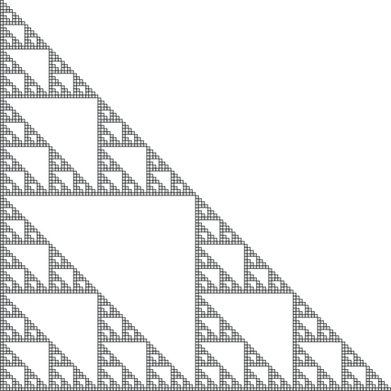
Figure 1: The standard discrete Sierpinski triangle $\mathbf{S}.$

We briefly review the standard discrete Sierpinski triangle and the calculation of its zeta-dimension.

Let $V=\{(1,0),(0,1)\}$. Define the sets $S_{0},S_{1},S_{2},\cdots\subseteq\mathbb{Z}^{2}$ by the recursion

$$S_{0}=\left\{\left(0,0\right)\right\},$$ (2.2)

$$S_{i+1}=S_{i}\cup\left(S_{i}+2^{i}V\right),$$

where $A+cB=\{\vec{m}+c\vec{n}|\vec{m}\in A\text{ and }\vec{n}\in B\}$. Then the standard discrete Sierpinski triangle is the set

$${\mathbf{S}}=\bigcup_{i=0}^{\infty}S_{i},$$

which is illustrated in Figure 1. It is well known that $\mathbf{S}$ is the set of all $(k,l)\in\mathbb{N}^{2}$ such that the binomial coefficient $\binom{k+l}{k}$ is odd. For this reason, the set $\mathbf{S}$ is also called Pascal’s triangle modulo 2. It is clear from the recursion (2.2) that $|S_{i}|=3^{i}$ for all $i\in\mathbb{N}$. The zeta-dimension of $\mathbf{S}$ is thus

$${\rm Dim}_{\zeta}(\mathbf{S}) = \limsup_{n\rightarrow\infty}\frac{\log\left|\mathbf{S}_{[0,2^{n}]}\right|}{n}$$

$$= \limsup_{n\rightarrow\infty}\frac{\log\left|S_{n}\right|}{n}$$

$$= \log 3$$

$$\approx 1.585.$$

3 Impossibility of Strict Self-Assembly of ${\rm{\bf{S}}}$

This section presents our first main theorem, which says that the standard discrete Sierpinski triangle $\bf{S}$ does not strictly self-assemble in the Tile Assembly Model. In order to prove this theorem, we first develop a lower bound on the number of tile types required for the self-assembly of a set $X$ in terms of the depths of finite trees that occur in a certain way as subtrees of the full grid graph $G^{\#}_{X}$ of $X$.

Intuitively, given a set $D$ of vertices of $G^{\#}_{X}$ (which is in practice the domain of the seed assembly), we now define a $D$-subtree of $G^{\#}_{X}$ to be any rooted tree in $G^{\#}_{X}$ that consists of all vertices of $G^{\#}_{X}$ that lie at or on the far side of the root from $D$. For simplicity, we state the definition in an arbitrary graph $G$.

Definition 19.

Let $G=(V,E)$ be a graph, and let $D\subseteq V$.

1. For each $r\in V$, the $D$-$r$-rooted subgraph of $G$ is the graph $G_{D,r}=\left(V_{D,r},E_{D,r}\right)$, where

   $$V_{D,r}=\left\{v\in V\left|\textmd{ every path from }v\textmd{ to (any vertex in) }D\textmd{ goes through }r\right.\right\}$$

   and

   $$E_{D,r}=E\cap\left[V_{D,r}\right]^{2}.$$

   (Note that $r\in V_{D,r}$ in any case.)

2. A $D$-subtree of $G$ is a rooted tree $B$ with root $r\in V$ such that $B=G_{D,r}$.

3. A branch of a $D$-subtree $B$ of $G$ is a simple path $\pi=\left(v_{0},v_{1},\ldots\right)$ in $B$ that starts at the root of $B$ and either ends at a leaf of $B$ or is infinitely long.

We use the following quantity in our lower bound theorem.

Definition 20.

Let $G=(V,E)$ be a graph, and let $D\subseteq V$. The finite-tree depth of $G$ relative to $D$ is

$$\textrm{ft-depth}_{D}\left(G\right)=\sup\left\{\textmd{depth(B)}\mid B\textmd{ is a finite }D\textmd{-subtree of }G\right\}.$$

We emphasize that the above supremum is only taken over finite $D$-subtrees. It is easy to construct an example in which $G$ has a $D$-subtree of infinite depth, but $\textrm{ft-depth}_{D}\left(G\right)<\infty$.

To prove our lower bound result, we use the following theorem from [2].

Theorem 3.1.

(Adleman, Cheng, Goel, Huang, Kempe, Moisset de Espanés, and Rothemund [2]) Let $X\subseteq\mathbb{Z}^{2}$ with $|X|<\infty$ be such that $G^{\#}_{X}$ is a tree rooted at the origin. If $X$ strictly self-assembles in a GTAS $\mathcal{T}=(T,\sigma,2)$ whose seed $\sigma$ consists of a single tile at the origin, then $|T|\geq\textrm{depth}\left(G^{\#}_{X}\right)$.

Our lower bound result is the following.

Theorem 3.2.

Let $X\subseteq\mathbb{Z}^{2}$. If $X$ strictly self-assembles in a GTAS $\mathcal{T}=(T,\sigma,\tau)$, then

$$|T|\geq\textrm{ft-depth}_{{\rm dom}\;{\sigma}}\left(G^{\#}_{X}\right).$$

Proof.

Assume the hypothesis, and let $B$ be a finite ${\rm dom}\;{\sigma}$-subtree of $G^{\#}_{X}$. If suffices to prove that $|T|\geq\textmd{depth}(B)$.

Let $\alpha\in\mathcal{A}_{\Box}\left[\mathcal{\mathcal{T}}\right]$, and let $\vec{r}$ be the root of $B$. Let $\sigma^{\prime}$ be the assembly with ${\rm dom}\;{\sigma^{\prime}}=\{\vec{r}\}$ and $\vec{u}\in U_{2}$. We define $\sigma^{\prime}(\vec{r})$ as follows.

$$\sigma^{\prime}(\vec{r})(\vec{u})=\left\{\begin{array}[]{ll}\left({\rm col}_{\alpha(\vec{r})}(\vec{u}),{\rm str}_{\alpha(\vec{r})}(\vec{u})\right)&\textrm{ if }\vec{r}+\vec{u}\in B\\ ({\rm col}_{\alpha(\vec{r})}(\vec{u}),0)&\textrm{ otherwise.}\end{array}\right.$$

Then $\mathcal{T}^{\prime}=(T,\sigma^{\prime},\tau)$ is a GTAS in which $B$ self-assembles. By Theorem 3.1, this implies that $|T|\geq\textmd{depth}(B)$. ∎

We next show that the standard discrete Sierpinski triangle $\bf{S}$ has infinite finite-tree depth.

Lemma 3.3.

For every finite set $D\subseteq S$, $\textrm{ft-depth}_{D}\left(G^{\#}_{\textbf{S}}\right)=\infty$.

Proof.

Let $D\subseteq\bf{S}$ be finite, and let $m$ be a positive integer. It suffices to show that $\textrm{ft-depth}_{D}\left(G^{\#}_{\textbf{S}}\right)>m$. Choose $k\in\mathbb{N}$ large enough to satisfy the following two conditions.

1. $2^{k}>\max\{a\in\mathbb{N}|(\exists b\in\mathbb{N})(a,b)\in D\}$.

2. $2^{k}>m$.

Let $\vec{r}_{k}=(2^{k+1},2^{k})$, and let

$$B_{k}=\left\{(a,b)\in\textbf{S}\left|a\geq 2^{k+1},b\geq 2^{k}\textrm{ and }a+b\leq 2^{k+2}-1\right.\right\}.$$

It is routine to verify that $G^{\#}_{B_{k}}$ is a finite $D$-subtree of $G^{\#}_{\bf{S}}$ with root at $\vec{r}$ and depth $2^{k}$. It follows that

$$\textrm{ft-depth}_{D}\left(G^{\#}_{\textbf{S}}\right)\geq\textmd{depth}\left(G^{\#}_{B_{k}}\right)=2^{k}>m.$$

∎

We now have the machinery to prove our first main theorem.

Theorem 3.4.

$\bf{S}$ does not strictly self-assemble in the Tile Assembly Model.

Proof.

Let $\mathcal{T}=(T,\sigma,\tau)$ be a GTAS in which $\bf{S}$ strictly self-assembles. It suffices to show that $\mathcal{T}$ is not a TAS. If ${\rm dom}\;{\sigma}$ is infinite, this is clear, so assume that ${\rm dom}\;{\sigma}$ is finite. Then Theorem 3.2 and Lemma 3.3 tell us that $|T|=\infty$, whence $\mathcal{T}$ is not a TAS. ∎

Before moving on, we note that Theorem 3.4 implies the following lower bound on the number of tile types needed to strictly assemble any finite stage $S_{n}$ of $\bf{S}$.

Corollary 3.5.

If a stage $S_{n}$ of $\bf{S}$ strictly self-assembles in a TAS $\mathcal{T}=(T,\sigma,\tau)$ in which $\sigma$ consists of a single tile at the origin, then $|T|\geq 2^{n}$.

If we let $N=\left|S_{n}\right|=3^{n}$, then the above lower bound exceeds $N^{0.63}$. As Rothemund [12] has noted, a structure of $N$ tiles that requires $\sqrt{N}$ or more tile types for its self-assembly cannot be said to feasibly self-assemble.

4 The Fibered Sierpinski Triangle ${\rm{{\bf T}}}$

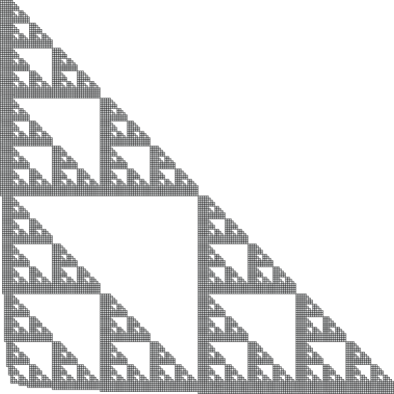
Figure 2: The fibered Sierpinski triangle $\mathbf{T}.$

We now define the fibered Sierpinski triangle and show that it has the same zeta-dimension as the standard discrete Sierpinski triangle.

As in Section 2, let $V=\{(1,0),(0,1)\}$. Our objective is to define sets of points $T_{0},T_{1},T_{2},\cdots\subseteq\mathbb{Z}^{2}$, sets $F_{0},F_{1},F_{2},\cdots\subseteq\mathbb{Z}^{2}$, and functions $l,f,t:\mathbb{N}\rightarrow\mathbb{N}$ with the following intuitive meanings.

1. $T_{i}$ is the $i^{\rm{th}}$ stage of our construction of the fibered Sierpinski triangle.

2. $F_{i}$ is the fiber associated with $T_{i}$, a thin strip of tiles along which data moves in the self-assembly process of Section 5. It is the smallest set whose union with $T_{i}$ has a vertical left edge and a horizontal bottom edge, together with one additional layer added to these two now-straight edges.

3. $l(i)$ is the length of (number of tiles in) the left (or bottom) edge of $T_{i}\cup F_{i}$.

4. $f(i)=\left|F_{i}\right|$.

5. $t(i)=\left|T_{i}\right|$.

These five entities are defined recursively by the equations

$$T_{0}=S_{2}\text{ (stage 2 in the construction of $S$)},$$

$$F_{0}=\left(\left\{-1\right\}\times\left\{-1,0,1,2,3\right\}\right)\cup\left(\left\{-1,0,1,2,3\right\}\times\left\{-1\right\}\right),$$

$$l(0)=5,$$

$$f(0)=9,$$

$$t(0)=9,$$

$$T_{i+1}=T_{i}\cup\left(\left(T_{i}\cup F_{i}\right)+l(i)V\right),$$ (4.1)

$$F_{i+1}=F_{i}\cup\left(\left\{-i-2\right\}\times\left\{-i-2,-i-1,\cdots,l(i+1)-i-3\right\}\right)$$

$$\cup\left(\left\{-i-2,-i-1,\cdots,l(i+1)-i-3\right\}\times\left\{-i-2\right\}\right),$$ (4.2)

$$l(i+1)=2l(i)+1,$$

$$f(i+1)=f(i)+2l(i+1)-1,$$

$$t(i+1)=3t(i)+2f(i).$$

Comparing the recursions (2.1) and (4.1) shows that the sets $T_{0},T_{1},T_{2},\cdots$ are constructed exactly like the sets $S_{0},S_{1},S_{2},\cdots$, except that the fibers $F_{i}$ are inserted into the construction of the sets $T_{i}$. A routine induction verifies that this recursion achieves conditions 2, 3, 4, and 5 above. The fibered Sierpinski triangle is the set

$${\mathbf{T}}=\bigcup_{i=0}^{\infty}T_{i}$$ (4.3)

which is illustrated in Figure 2. The resemblance between ${\mathbf{S}}$ and ${\mathbf{T}}$ is clear from the illustrations. We now verify that ${\mathbf{S}}$ and ${\mathbf{T}}$ have the same zeta-dimension.

Lemma 4.1.

$\textmd{Dim}_{\zeta}(\bf{T})=\textmd{Dim}_{\zeta}(\bf{S})$.

Proof.

Solving the recurrences for $l$, $f$, and $t$, in that order, gives the formulas

$$l(i)=3\cdot 2^{i+1}-1,$$

$$f(i)=3\left(2^{i+3}-i-5\right),$$

$$t(i)=\frac{3}{2}\left(3^{i+3}-2^{i+5}+2i+11\right),$$

which can be routinely verified by induction. It follows readily that

$${\rm Dim}_{\zeta}\left(\mathbf{T}\right)=\limsup_{n\rightarrow\infty}\frac{\log t(n)}{\log l(n)}=\log 3={\rm Dim}_{\zeta}\left(\mathbf{S}\right).$$

∎

We note that the thickness $i+1$ of a fiber $F_{i}$ is $O(\log l(i))$, i.e., logarithmic in the side length of $T_{i}$. Hence the difference between $S_{i}$ and $T_{i}$ is asymptotically negligible as $i\rightarrow\infty$. Nevertheless, we show in the next section that $\mathbf{T}$, unlike $\mathbf{S}$, strictly self-assembles in the Tile Assembly Model.

5 Strict Self-Assembly of $\bf{T}$

This section is devoted to proving our second main theorem, which is the fact that the fibered Sierpinski triangle $\bf{T}$ strictly self-assembles in the Tile Assembly Model. Our proof is constructive, i.e., we exhibit a specific tile assembly system in which $\bf{T}$ strictly self-assembles.

Our strict self-assembly of $\bf{T}$ is not based directly upon the recursive definition (4.1). A casual inspection of Figure 2 suggests that $\bf{T}$ can also be regarded as a structure consisting of many horizontal and vertical bars, with each large bar having many smaller bars perpendicular to it. In subsection 5.1 we give a precise statement and proof of this “bar characterization” of $\bf{T}$, which is the basis of our strict self-assembly. In subsections 5.2 and 5.3 we present the main functional subsystems of our construction. This gives us a tile assembly system $\mathcal{T}_{\bf{T}}=(T_{\mathbf{T}},\sigma_{\mathbf{T}},\tau)$, where

1. the tile set $T_{\mathbf{T}}$ consists of 51 tile types;

2. the seed assembly $\sigma_{\mathbf{T}}$ consists of a single ‘S’ tile at the origin; and

3. the temperature $\tau$ is 2.

Subsection 5.4 proves that the fibered Sierpinski triangle $\bf{T}$ strictly
self-assembles in $\mathcal{T}_{\bf{T}}$.

Throughout this section, the temperature $\tau$ is 2. Tiles are depicted as squares whose various sides are dotted lines, solid lines, or doubled lines, indicating whether the glue strengths on these sides are 0, 1, or 2, respectively. Thus, for example, a tile of the type shown in Figure 3

Figure 3: An example tile type.

has glue of strength 0 on the left and bottom, glue of color ‘a’ and strength 2 on the top, and glue of color ‘b’ and strength 1 on the right. This tile also has a label ‘L’, which plays no formal role but may aid our understanding and discussion of the construction.

5.1 Bar Characterization of $\bf{T}$

We now formulate the characterization of $\bf{T}$ that guides its strict self-assembly. At the outset, in the notation of section 4, we focus on the manner in which the sets $T_{i}\cup F_{i}$ can be constructed from horizontal and vertical bars. Recall that

$$l(i)=3\cdot 2^{i+1}-1$$

is the length of (number of tiles in) the left or bottom edge of $T_{i}\cup F_{i}$.

Definition 21.

Let $-1\leq i\in\mathbb{Z}$.

1. The $S_{i}$-square is the set

   $$S_{i}=\{-i-1,\ldots,0\}\times\{-i-1,\ldots,0\}.$$

2. The $X_{i}$-bar is the set

   $$X_{i}=\{1,\ldots,l(i)-i-2\}\times\{-i-1,\ldots,0\}.$$

3. The $Y_{i}$-bar is the set

   $$Y_{i}=\{-i-1,\ldots,0\}\times\{1,\ldots,l(i)-i-2\}.$$

It is clear that the set

$$S_{i}\cup X_{i}\cup Y_{i}$$

is the “outer framework” of $T_{i}\cup F_{i}$. Our attention thus turns to the manner in which smaller and smaller bars are recursively attached to this framework.

We use the ruler function

$$\rho:\mathbb{Z}^{+}\rightarrow\mathbb{N}$$

defined by the recurrence

$$\rho(2k+1) = 0,$$

$$\rho(2k) = \rho(k)+1$$

for all $k\in\mathbb{N}$. It is easy to see that $\rho(n)$ is the (exponent of the) largest power of 2 that divides $n$. Equivalently, $\rho(n)$ is the number of 0’s lying to the right of the rightmost 1 in the binary expansion of $n$ [9]. An easy induction can be used to establish the following observation.

Observation 5.1.

For all $n\in\mathbb{N}$,

$$\sum_{j=1}^{2^{n+1}-1}{\rho(j)}=2^{n+1}-n-2.$$

Using the ruler function, we define the function

$$\theta:\mathbb{Z}^{+}\rightarrow\mathbb{Z}^{+}$$

by the recurrence

$$\theta(1) = 2,$$

$$\theta(j+1) = \theta(j)+\rho(j+1)+2$$

for all $j\in\mathbb{Z}^{+}$.

We now use the function $\theta$ to define the points at which smaller bars are attached to the $X_{i}$- and $Y_{i}$-bars.

Definition 22.

1. The $j^{\textmd{th}}$ $\theta$-point of $X_{i}$ is the point

   $$\theta_{j}(X_{i})=(\theta(j),1),$$

   lying just above the $X_{i}$-bar.

2. The $j^{\textmd{th}}$ $\theta$-point of $Y_{i}$ is the point

   $$\theta_{j}(Y_{i})=(1,\theta(j)),$$

   lying just to the right of the $Y_{i}$-bar.

The following recursion attaches smaller bars to larger bars in a recursive fashion.

Definition 23.

The $\theta$-closures of the bars $X_{i}$ and $Y_{i}$ are the sets $\theta(X_{i})$ and $\theta(Y_{i})$ defined by the mutual recursion

$$\theta\left(X_{-1}\right) = X_{-1}$$

$$\theta\left(Y_{-1}\right) = Y_{-1}$$

$$\theta(X_{i}) = X_{i}\cup\bigcup_{j=1}^{2^{i+1}-1}{\left(\theta_{j}(X_{i})+\theta\left(Y_{\rho(j)-1}\right)\right)},$$

$$\theta(Y_{i}) = Y_{i}\cup\bigcup_{j=1}^{2^{i+1}-1}{\left(\theta_{j}(Y_{i})+\theta\left(X_{\rho(j)-1}\right)\right)},$$

for all $i\in\mathbb{N}$.

This definition, along with the symmetry of $\rho$, admit the following characterizations of $\theta(X_{i})$ and $\theta(Y_{i})$.

Observation 5.2.

Let $0\leq i\in\mathbb{N}$.

1. $$\theta\left(X_{i+1}\right) = \theta(X_{i})\cup\left(\left(S_{i}\cup\theta(X_{i})\cup\theta(Y_{i})\right)+(l(i),0)\right)$$

   $$\quad\cup\left(\{1,\ldots l(i+1)-i-3\}\times\{-i-2\}\right)$$

2. $$\theta\left(Y_{i+1}\right) = \theta(Y_{i})\cup\left(\left(S_{i}\cup\theta(X_{i})\cup\theta(Y_{i})\right)+(0,l(i))\right)$$

   $$\quad\cup\left(\{-i-2\}\times\{1,\ldots l(i+1)-i-3\}\right)$$

We have the following characterization of the sets $T_{i}\cup F_{i}$.

Lemma 5.3.

For all $i\in\mathbb{N}$,

$$T_{i}\cup F_{i}=S_{i}\cup\theta(X_{i})\cup\theta(Y_{i}).$$

Proof.

We proceed by induction on $i$, and note that the case when $i=0$ is trivial. Assume that, for all $i\in\mathbb{N}$, the lemma holds. Then we have

$$T_{i+1}\cup F_{i+1} \stackrel{{\scriptstyle\textmd{(4.1)}}}{{=}} T_{i}\cup\left(\left(T_{i}\cup F_{i}\right)+l(i)V\right)\cup F_{i+1}$$

$$\stackrel{{\scriptstyle\textmd{(4.2)}}}{{=}} \left(T_{i}\cup F_{i}\right)\cup\left(\left(T_{i}\cup F_{i}\right)+l(i)V\right)\cup$$

$$\quad\left(\{-i-2\}\times\{-i-2,\ldots,l(i+1)-i-3\}\right)\cup$$

$$\quad\quad\left(\{-i-2,\ldots,l(i+1)-i-3\}\times\{-i-2\}\right)$$

$$\stackrel{{\scriptstyle\textmd{Ind Hyp}}}{{=}} \left(S_{i}\cup\theta(X_{i})\cup\theta(Y_{i})\right)\cup\left(\left(S_{i}\cup\theta(X_{i})\cup\theta(Y_{i})\right)+l(i)V\right)\cup$$

$$\quad\left(\{-i-2\}\times\{-i-2,\ldots,l(i+1)-i-3\}\right)\cup$$

$$\quad\quad\left(\{-i-2,\ldots,l(i+1)-i-3\}\times\{-i-2\}\right)$$

$$\stackrel{{\scriptstyle\textmd{Observation 5.2}}}{{=}} S_{i+1}\cup\theta(X_{i+1})\cup\theta(Y_{i+1}).$$

∎

We now shift our attention to the global structure of the set $\bf{T}$.

Definition 24.

1. The $x$-axis of $\bf{T}$ is the set

   $$X=\{(m,n)\in\mathbf{T}\;|\;m>0,\textmd{ and }n\leq 0\}.$$

2. The $y$-axis of $\mathbf{T}$ is the set

   $$Y=\{(m,n)\in\mathbf{T}\;|\;m\leq 0,\textmd{ and }n>0\}.$$

Intuitively, the $x$-axis of $\bf{T}$ is the part of $\bf{T}$ that is a “gradually thickening bar” lying on and below the (actual) $x$-axis in $\mathbb{Z}^{2}$. (see Figure 2.) For technical convenience, we have omitted the origin from this set. Similar remarks apply to the $y$-axis of $\bf{T}$.

Define the sets

$$\widetilde{X}_{-1} = \{(1,0),(2,0),(3,0)\},$$

$$\widetilde{Y}_{-1} = \{(0,1),(0,2),(0,3)\}.$$

For each $i\in\mathbb{N}$, define the translations

$$S_{i}^{\rightarrow} = (l(i),0)+S_{i},$$

$$S_{i}^{\uparrow} = (0,l(i))+S_{i},$$

$$X_{i}^{\rightarrow} = (l(i),0)+X_{i},$$

$$Y_{i}^{\uparrow} = (0,l(i))+Y_{i}$$

of $S_{i}$, $X_{i}$, and $Y_{i}$. It is clear by inspection that $X$ is the disjoint union of the sets

$$\widetilde{X}_{-1},S_{0}^{\rightarrow},X_{0}^{\rightarrow},S_{1}^{\rightarrow},X_{1}^{\rightarrow},S_{2}^{\rightarrow},X_{2}^{\rightarrow},\ldots,$$

which are written in their left-to-right order of position in $X$. More succinctly, we have the following.

Observation 5.4.

1. $\displaystyle X=\widetilde{X}_{-1}\cup\bigcup_{i=0}^{\infty}{\left(S_{i}^{\rightarrow}\cup X_{i}^{\rightarrow}\right)}$.

2. $\displaystyle Y=\widetilde{Y}_{-1}\cup\bigcup_{i=0}^{\infty}{\left(S_{i}^{\uparrow}\cup Y_{i}^{\uparrow}\right)}$.

Moreover, both of these are disjoint unions.

In light of Observation 5.4, it is convenient to define, for each $-1\leq n\in\mathbb{Z}$, the initial segment

$$\widetilde{X}_{n}=\widetilde{X}_{-1}\cup\bigcup_{i=0}^{n}{\left(S_{i}^{\rightarrow}\cup X_{i}^{\rightarrow}\right)}$$

of $X$ and the initial segment

$$\widetilde{Y}_{n}=\widetilde{Y}_{-1}\cup\bigcup_{i=0}^{n}{\left(S_{i}^{\uparrow}\cup Y_{i}^{\uparrow}\right)}$$

of $Y$. (Note that this is consistent with earlier usage when $n=-1$.)

The following definition specifies the manner in which bars are recursively attached to the $x$- and $y$-axes of $\bf{T}$.

Definition 25.

Let $j\in\mathbb{Z}^{+}$.

1. The $j^{\textmd{th}}$ $\theta$-point of $X$ is the point

   $$\theta_{j}(X)=(\theta(j),1)$$

   lying just above $X$.

2. The $j^{\textmd{th}}$ $\theta$-point of $Y$ is the point

   $$\theta_{j}(Y)=(1,\theta(j))$$

   lying just to the right of $Y$.

Definition 26.

For all $-1\leq n\in\mathbb{Z}$, the $\theta$-closures of the initial segment of the axes $\widetilde{X}_{n}$ and $\widetilde{Y}_{n}$ are the sets

$$\theta\left(\widetilde{X}_{n}\right)=\widetilde{X}_{n}\cup\bigcup_{j=1}^{2^{n+2}-1}{\left(\theta_{j}\left(X\right)+\theta\left(Y_{\rho(j)-1}\right)\right)}$$

and

$$\theta\left(\widetilde{Y}_{n}\right)=\widetilde{Y}_{n}\cup\bigcup_{j=1}^{2^{n+2}-1}{\left(\theta_{j}(Y)+\theta\left(X_{\rho(j)-1}\right)\right)},$$

respectively.

The following observation is an immediate consequence of the previous definition.

Observation 5.5.

Let $0\leq n\in\mathbb{N}$.

1. $\theta\left(\widetilde{X}_{n}\right)=\theta\left(\widetilde{X}_{n-1}\right)\cup\left(\left(S_{n}\cup\theta\left(X_{n}\right)\cup\theta\left(Y_{n}\right)\right)+(l(n),0)\right)$.

2. $\theta\left(\widetilde{Y}_{n}\right)=\theta\left(\widetilde{Y}_{n-1}\right)\cup\left(\left(S_{n}\cup\theta\left(X_{n}\right)\cup\theta\left(Y_{n}\right)\right)+(0,l(n))\right)$.

We have the following characterization of $T_{n}$.

Lemma 5.6.

For all $-1\leq n\in\mathbb{Z}$,

$$T_{n+1}=\{(0,0)\}\cup\theta\left(\widetilde{X}_{n}\right)\cup\theta\left(\widetilde{Y}_{n}\right).$$

Proof.

We proceed by induction on $n$. When $n=-1$, it is easy to see that

$$\{(0,0)\}\cup\theta\left(\widetilde{X}_{-1}\right)\cup\theta\left(\widetilde{Y}_{-1}\right)=T_{0}.$$

Now assume that, for all $-1\leq n\in\mathbb{N}$, the lemma holds. Then we have

$$T_{n+2} \stackrel{{\scriptstyle\textmd{(4.1)}}}{{=}} T_{n+1}\cup\left(\left(T_{n+1}\cup F_{n+1}\right)+l(n+1)V\right)$$

$$\stackrel{{\scriptstyle\textmd{Ind Hyp}}}{{=}} \left(\{(0,0)\}\cup\theta\left(\widetilde{X}_{n}\right)\cup\theta\left(\widetilde{Y}_{n}\right)\right)\cup$$

$$\quad\left(\left(T_{n+1}\cup F_{n+1}\right)+l(n+1)V\right)$$

$$\stackrel{{\scriptstyle\textmd{Lemma 5.3}}}{{=}} \left(\{(0,0)\}\cup\theta\left(\widetilde{X}_{n}\right)\cup\theta\left(\widetilde{Y}_{n}\right)\right)\cup$$

$$\quad\left(\left(S_{n+1}\cup\theta\left(X_{n+1}\right)\cup\theta\left(Y_{n+1}\right)\right)+l(n+1)V\right)$$

$$\stackrel{{\scriptstyle\textmd{Observation 5.5}}}{{=}} \{(0,0)\}\cup\theta\left(\widetilde{X}_{n+1}\right)\cup\theta\left(\widetilde{Y}_{n+1}\right).$$

∎

Definition 27.

The $\theta$-closures of the axes $X$ and $Y$ are the sets

$$\theta(X)=X\cup\bigcup_{j=1}^{\infty}{\left(\theta_{j}(X)+\theta\left(Y_{\rho(j)-1}\right)\right)}$$

and

$$\theta(Y)=Y\cup\bigcup_{j=1}^{\infty}{\left(\theta_{j}(Y)+\theta\left(X_{\rho(j)-1}\right)\right)},$$

respectively.

Figure 3 shows the structure of the $Y$-axis.

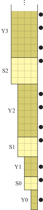
Figure 4: The structure of $Y$. The dots denote the $\theta$-points.

Lemma 5.7.

Let $\-1\leq i\in\mathbb{Z}$.

1. $\theta(X)=\displaystyle\bigcup_{i=-1}^{\infty}{\theta\left(\widetilde{X}_{i}\right)}$.

2. $\theta(Y)=\displaystyle\bigcup_{i=-1}^{\infty}{\theta\left(\widetilde{Y}_{i}\right)}$.

Proof.

For all $-1\leq i\in\mathbb{Z}$, it follows from the definition of $\theta\left(\widetilde{X}_{i}\right)$, that

$$\bigcup_{i=-1}^{\infty}{\theta\left(\widetilde{X}_{i}\right)} = \bigcup_{i=-1}^{\infty}{\left(\widetilde{X}_{i}\cup\bigcup_{j=1}^{2^{i+2}-1}{\left(\theta_{j}(X)+\theta\left(Y_{\rho(j)-1}\right)\right)}\right)}$$

$$= \left(\bigcup_{i=-1}^{\infty}{\widetilde{X}_{i}}\right)\cup\bigcup_{i=-1}^{\infty}{\bigcup_{j=1}^{2^{i+2}-1}{\left(\theta_{j}(X)+\theta\left(Y_{\rho(j)-1}\right)\right)}}$$

$$\stackrel{{\scriptstyle\textmd{Observation 5.4}}}{{=}} X\cup\bigcup_{i=1}^{\infty}{\left(\theta_{j}(X)+\theta\left(Y_{\rho(j)-1}\right)\right)}$$

$$= \theta(X).$$

The proof of (2) is similar. ∎

We now have the following characterization of the fibered Sierpinski triangle.

Theorem 5.8 (bar characterization of $\mathbf{T}$).

$$\mathbf{T}=\{(0,0)\}\cup\theta(X)\cup\theta(Y).$$

Proof.

$$\mathbf{T} \stackrel{{\scriptstyle\textmd{(4.3)}}}{{=}} \bigcup_{i=0}^{\infty}{T_{i}}$$

$$\stackrel{{\scriptstyle\textmd{Lemma 5.6}}}{{=}} \bigcup_{i=-1}^{\infty}{\left(\{(0,0)\}\cup\theta\left(\widetilde{X}_{i}\right)\cup\theta\left(\widetilde{Y}_{i}\right)\right)}$$

$$= \{(0,0)\}\cup\bigcup_{i=-1}^{\infty}{\left(\theta\left(\widetilde{X}_{i}\right)\cup\theta\left(\widetilde{Y}_{i}\right)\right)}$$

$$= \{(0,0)\}\cup\bigcup_{i=-1}^{\infty}{\theta\left(\widetilde{X}_{i}\right)}\cup\bigcup_{i=-1}^{\infty}{\theta\left(\widetilde{Y}_{i}\right)}$$

$$\stackrel{{\scriptstyle\textmd{Lemma 5.7}}}{{=}} \{(0,0)\}\cup\theta(X)\cup\theta(Y).$$

∎

In the following subsections, we use Theorem 5.8 to guide the strict self-assembly of $\bf{T}$.

5.2 Self-Assembly of the Axes

In this subsection, we exhibit a TAS in which the $y$-axis of $\mathbf{T}$ strictly self-assembles. Our tile set is a modification of the optimal binary counter (see [5]). If $i+2\in\mathbb{N}$ is the width of our modified binary counter, then every number $1\leq j\leq 2^{i+1}$ is counted once, and then, if $j\neq 2^{i+1}$, copied $\rho(j)+1$ times. It is easy to verify, using Observation 5.1, that this counting scheme produces a rectangle having a width of $i+2$, and a height of

$$2^{i+1}+\sum_{j=1}^{2^{i+1}-1}{\left(\rho(j)+1\right)}=l(i)-i-2,$$

which is precisely the set $Y_{i}$.

We will now construct our set of tile types $T$.

Construction 5.9.

Let $T$ be the set of 25 tile types shown in Figure 5.

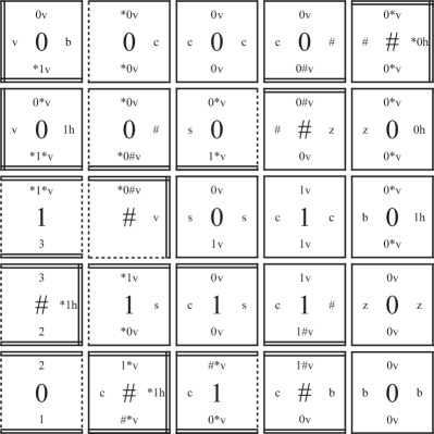
Figure 5: The set of tile types in which the set $Y$ self-assembles.

The following technical result gives an assembly sequence for the set $Y_{i}-(\{-i-1\}\times\{1,\ldots,l(i)-i-2\})$.

Lemma 5.10.

Let $n\in\mathbb{N}$. If, for some $m\in\mathbb{Z}$, $\sigma_{n}\in\mathcal{A}^{\tau}_{T}$ satisfies

1. $\displaystyle{\rm dom}\;{\sigma_{n}}=\left(\{-n-1,\ldots,0\}\times\{m-1,m\}\right)$,

2. for all $\vec{v}\in\left(\{-n-1,\ldots,0\}\times\{m\}\right)$,

   $$\sigma_{n}\left(\vec{v}\right)(0,1)=\left\{\begin{array}[]{ll}\left(\textmd{0*v},2\right)&\textmd{if }\vec{v}=(0,m)\\ \left(\textmd{0v},1\right)&\textmd{if }\vec{v}\neq(0,m)\textmd{ and }\vec{m}\neq(-n-1,m),\\ \end{array}\right.$$

then there is a $\tau$-$T$-assembly sequence $\vec{\alpha}_{n}=\left(\alpha_{i_{n}}\left|\;0\leq i_{n}<k_{n}<\infty\right.\right)$, with $\alpha=\textrm{res}(\vec{\alpha}_{n})$, satisfying

1. $\alpha_{0_{n}}=\sigma_{n}$,

2. ${\rm dom}\;{\alpha}={\rm dom}\;{\sigma_{n}}\cup\left(\left(Y_{n}-\left(\{-n-1\}\times\{1,\ldots,l(n)-n-2\}\right)\right)+(0,m)\right)$,

3. for all $\vec{v}\in{\rm dom}\;{\alpha}-{\rm dom}\;{\sigma_{n}}$,

   $$\sum_{\vec{u}\in\textmd{IN}^{\vec{\alpha}}(\vec{v})}{\textmd{str}_{\alpha_{i_{\vec{\alpha}}(\vec{v})}}(\vec{v},\vec{u})}=\tau,$$

4. for all $\vec{v}\in{\rm dom}\;{\alpha}-{\rm dom}\;{\sigma_{n}}$ and all $t\in T-\{\alpha(\vec{v})\}$, $\vec{v}\not\in{\partial}^{\tau}_{t}{\left(\vec{\alpha}\setminus\vec{v}\right)}$,

5. for all $\vec{v}\in{\rm dom}\;{\alpha}-{\rm dom}\;{\sigma_{n}}$,

   $$\alpha\left(\vec{v}\right)(1,0)=\left\{\begin{array}[]{ll}\left(\textmd{*1h},2\right)&\textmd{if }\exists j\in\mathbb{N},\textmd{ and }\vec{v}=(0,\theta(2j+1)+m)\\ \left(\textmd{*0h},2\right)&\textmd{if }\exists j\in\mathbb{N},\textmd{ and }\vec{v}=(0,\theta(2j)+m)\\ \left(\textmd{0h},1\right)&\textmd{if }\exists j\in\mathbb{N},\textmd{ and }\\ &\vec{v}\in(\left(\{0\}\times\{\theta\left(j\right)-\rho\left(j\right)+1,\ldots,\theta\left(j\right)-1\}\right)\\ &\quad+(0,m))\\ \left(\textmd{1h},1\right)&\textmd{if }\exists j\in\mathbb{N},\textmd{ and }\vec{v}=(0,\theta(j)-\rho(j)+m)\\ \left(\lambda,0\right)&\textmd{otherwise,}\\ \end{array}\right.$$

   and

6. for all $\vec{v}\in\left\{(x,y)\in{\rm dom}\;{\alpha}\left|\;(x,y+1)\not\in{\rm dom}\;{\alpha}\right.\right\}$,

   $$\alpha\left(\vec{v}\right)(0,1)=\left\{\begin{array}[]{ll}\left(\textmd{0*v},1\right)&\textmd{if }\vec{v}+(1,0)\not\in{\rm dom}\;{\alpha}\\ \left(\textmd{0v},1\right)&\textmd{otherwise.}\end{array}\right.$$

Proof.

We proceed by induction on $n$, noting that the the base case is verified in Figure 6.

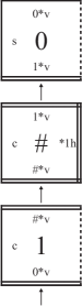
Figure 6: The base case for Lemma 5.10.

Now assume that the claim holds for all $n\in\mathbb{N}$, and let $\sigma_{n+1}\in\mathcal{A}^{\tau}_{T}$ satisfy conditions (1) and (2) of the hypothesis, taking $m=0$. Let $\sigma_{n}\in\mathcal{A}^{\tau}_{T}$ satisfy, for all $\vec{v}\in\mathbb{Z}^{2}$,

$$\sigma_{n}(\vec{v})=\left\{\begin{array}[]{ll}\sigma_{n+1}(\vec{v})&\textmd{ if }\vec{v}\in(\{-n-1,\ldots,0\}\times\{-1,0\})\\ \uparrow&\textmd{ otherwise.}\\ \end{array}\right.$$

Then the induction hypothesis tells us that there is an assembly sequence $\vec{\alpha}_{n}$, with $\alpha=\textrm{res}(\vec{\alpha}_{n})$, satisfying conditions (1), (2), (3), (4), (5), and (6) of the conclusion, taking $m=0$. Define the assembly sequence

$$\vec{\alpha}_{n+1}=\left(\left.\alpha_{i_{n+1}}\;\right|\;0\leq i_{n+1}<k_{n+1}<\infty\right)$$

satisfying

1. $\alpha_{0_{n+1}}=\sigma_{n+1}$,

2. for all $0\leq i_{n+1}<k_{n}$, $\alpha_{i_{n+1}}=\alpha_{i_{n}}$,

3. for all $0\leq i<l(n)-n-3$, $\alpha_{\left(k_{n}+i\right)_{n+1}}=\alpha_{\left(k_{n}+i-1\right)_{n+1}}+((-n-1,i+1)\mapsto t)$, where $t$ is the tile type shown in Figure 7, and

   

   Figure 7: The tile type $t$.

4. $\displaystyle\alpha_{\left(k_{n}+l(n)-n-3\right)_{n+1}}=\alpha_{\left(k_{n}+l(n)-n-4\right)_{n+1}}+((-n-1,l(n)-n-2)\mapsto t^{\prime})$, where $t^{\prime}$ is the tile type shown in Figure 8.

   

   Figure 8: The tile type $t^{\prime}$.

Notice that for all

$$\vec{v}\in\left\{\left.(x,y)\in{\rm dom}\;{\alpha_{\left(k_{n}+l(n)-n-3\right)_{n+1}}}\;\right|\;(x,y+1)\not\in{\rm dom}\;{\alpha_{\left(k_{n}+l(n)-n-3\right)_{n+1}}}\right\}$$

,

$$\alpha_{\left(k_{n}+l(n)-n-3\right)_{n+1}}\left(\vec{v}\right)(0,1)=\left\{\begin{array}[]{ll}\left(\textmd{0v},2\right)&\textmd{if }\vec{v}+(-1,0)\not\in{\rm dom}\;{\alpha}\\ \left(\textmd{0*v},1\right)&\textmd{if }\vec{v}+(1,0)\not\in{\rm dom}\;{\alpha}\\ \left(\textmd{0v},1\right)&\textmd{otherwise.}\end{array}\right.$$

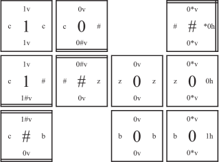
Figure 9: Tile types in which $S_{n}^{\uparrow}$ self-assembles.

The tile types shown in Figure 9 testify that there is a $\tau$-$T$-assembly sequence

$$\vec{\Box}=\left(\alpha_{\left(k_{n}+l(n)-n-2\right)_{n+1}},\ldots,\alpha_{\left(k_{n}+l(n)-n-2+(n+1)^{2}-1\right)_{n+1}}\right)$$

having the property that

$${\rm dom}\;{\alpha_{\left(k_{n}+l(n)-n-2+(n+1)^{2}-1\right)_{n+1}}}-{\rm dom}\;{\alpha_{\left(k_{n}+l(n)-n-2\right)_{n+1}}}=S_{n}^{\uparrow},$$

and for all $\vec{v}\in(\{-n-1,\ldots 0\}\times\{l(n)\})$,

$$\alpha_{\left(k_{n}+l(n)-n-2+(n+1)^{2}-1\right)_{n+1}}\left(\vec{v}\right)(0,1)=\left\{\begin{array}[]{ll}\left(\textmd{0*v},2\right)&\textmd{if }\vec{v}=(0,l(n))\\ \left(\textmd{1v},1\right)&\textmd{if }\vec{v}=(-n-1,l(n))\\ \left(\textmd{0v},1\right)&\textmd{otherwise.}\\ \end{array}\right.$$

Let $\sigma^{\prime}_{n}\in\mathcal{A}^{\tau}_{T}$ satisfy, for all $\vec{v}\in\mathbb{Z}^{2}$,

$$\sigma^{\prime}_{n}(\vec{v})=\left\{\begin{array}[]{ll}\alpha_{\left(k_{n}+l(n)-n-2+(n+1)^{2}-1\right)_{n+1}}(\vec{v})&\textmd{ if }\vec{v}\in(\{-n-1,\ldots,0\}\\ &\quad\times\{l(n)-1,l(n)\})\\ \uparrow&\textmd{ otherwise.}\\ \end{array}\right.$$

Once again, we appeal to the induction hypothesis, which tells us that there is an assembly sequence $\vec{\alpha}^{\prime}_{n}$, with $\alpha^{\prime}=\textrm{res}(\vec{\alpha}^{\prime}_{n})$, satisfying, with $m=l(n)$, conditions (1), (2), (3), (4), (5), and (6) of the conclusion. Thus, we can define an assembly sequence $\vec{\alpha}^{\prime}_{n+1}=\left(\left.\alpha_{i^{\prime}_{n+1}}\;\right|\;0\leq i^{\prime}_{n+1}<k^{\prime}_{n+1}<\infty\right)$ satisfying

1. $\alpha_{0^{\prime}_{n+1}}=\alpha_{\left(k_{n}+l(n)-n-2+(n+1)^{2}-1\right)_{n+1}}$,

2. for all $1\leq i^{\prime}_{n+1}<k^{\prime}_{n}$, $\alpha_{i^{\prime}_{n+1}}=\alpha_{i^{\prime}_{n}}$,

3. for all $0\leq i<l(n)-n-2$,

   $$\alpha_{\left(k^{\prime}_{n}+i\right)_{n+1}}=\alpha_{\left(k^{\prime}_{n}+i-1\right)_{n+1}}+\left((-n-1,i+1+l(n))\mapsto t^{\prime\prime}\right),$$

   where $t^{\prime\prime}$ is the tile type shown in Figure 10, and

   

   Figure 10: The tile type $t^{\prime\prime}$.

4. $\displaystyle\alpha_{\left(k^{\prime}_{n}+l(n)-n-3\right)_{n+1}}=\alpha_{\left(k^{\prime}_{n}+l(n)-n-4\right)_{n+1}}+\left((-n-1,l(n+1)-n-3)\mapsto t^{\prime\prime\prime}\right)$, where $t^{\prime\prime\prime}$ is the tile type shown in Figure 11.

   

   Figure 11: The tile type $t^{\prime\prime\prime}$.

It is routine to verify that $\vec{\alpha}\cup\vec{\Box}\cup\vec{\alpha}^{\prime}$ is a $\tau$-$T$-assembly sequence satisfying conditions (1), (2), (3), (4), (5), and (6) of the conclusion. ∎

In the following, we assume the presence of $\widetilde{Y}_{n-1}\cup S_{n}^{\uparrow}$, and use Lemma 5.10 to give an assembly sequence for the set $Y_{i}^{\uparrow}$.

Lemma 5.11.

Let $n\in\mathbb{N}$. If $\sigma_{n}\in\mathcal{A}^{\tau}_{T}$ satisfies

1. $\displaystyle{\rm dom}\;{\sigma_{n}}=\left(\widetilde{Y}_{-1}\cup S_{0}^{\uparrow}\right)\cup\bigcup_{i=1}^{n}{\left(Y_{i-1}^{\uparrow}\cup S_{i}^{\uparrow}\right)}$, and

2. for all $\vec{m}\in\left\{(x,y)\in{\rm dom}\;{\sigma_{n}}\left|\;(x,y+1)\not\in{\rm dom}\;{\sigma_{n}}\right.\right\}$,

   $$\sigma_{n}\left(\vec{m}\right)(0,1)=\left\{\begin{array}[]{ll}\left(\textmd{*0v},1\right)&\textmd{if }\vec{m}+(-1,0)\not\in{\rm dom}\;{\sigma_{n}}\\ \left(\textmd{0*v},2\right)&\textmd{if }\vec{m}+(1,0)\not\in{\rm dom}\;{\sigma_{n}}\\ \left(\textmd{0v},1\right)&\textmd{otherwise},\end{array}\right.$$

then there is a $\tau$-$T$-assembly sequence $\vec{\alpha}=\left(\alpha_{i}\left|\;0\leq i<k<\infty\right.\right)$, with $\alpha=\textrm{res}(\vec{\alpha})$, satisfying

1. $\alpha_{0}=\sigma_{n}$,

2. ${\rm dom}\;{\alpha}=\widetilde{Y}_{n}$,

3. for all $\vec{m}\in{\rm dom}\;{\alpha}-{\rm dom}\;{\sigma_{n}}$,

   $$\sum_{\vec{u}\in\textmd{IN}^{\vec{\alpha}}(\vec{m})}{\textmd{str}_{\alpha_{i_{\vec{\alpha}}(\vec{m})}}(\vec{m},\vec{u})}=\tau,$$

4. for all $\vec{m}\in{\rm dom}\;{\alpha}-{\rm dom}\;{\sigma_{n}}$ and all $t\in T-\{\alpha(\vec{m})\}$, $\vec{m}\not\in{\partial}^{\tau}_{t}{\left(\vec{\alpha}\setminus\vec{m}\right)}$,

5. for all $\vec{m}\in{\rm dom}\;{\alpha}-{\rm dom}\;{\sigma_{n}}$,

   $$\alpha\left(\vec{m}\right)(1,0)=\left\{\begin{array}[]{ll}\left(\textmd{*1h},2\right)&\textmd{if }\exists j\in\mathbb{N},\textmd{ and }\vec{m}=(0,\theta(2j+1))\\ \left(\textmd{*0h},2\right)&\textmd{if }\exists j\in\mathbb{N},\textmd{ and }\vec{m}=(0,\theta(2j))\\ \left(\textmd{0h},1\right)&\textmd{if }\exists j\in\mathbb{N},\textmd{ and }\\ &\quad\vec{m}\in\left(\{0\}\times\{\theta\left(j\right)-\rho\left(j\right)+1,\ldots,\theta\left(j\right)-1\}\right)\\ \left(\textmd{1h},1\right)&\textmd{if }\exists j\in\mathbb{N},\textmd{ and }\vec{m}=(0,\theta(j)-\rho(j))\\ \left(\lambda,0\right)&\textmd{otherwise,}\\ \end{array}\right.$$

   and

6. for all $\vec{m}\in\left\{(x,y)\in{\rm dom}\;{\alpha}\left|\;(x,y+1)\not\in{\rm dom}\;{\alpha}\right.\right\}$,

   $$\alpha\left(\vec{m}\right)(0,1)=\left\{\begin{array}[]{ll}\left(\textmd{*1v},2\right)&\textmd{if }\vec{m}+(-1,0)\not\in{\rm dom}\;{\alpha}\\ \left(\textmd{0*v},1\right)&\textmd{if }\vec{m}+(1,0)\not\in{\rm dom}\;{\alpha}\\ \left(\textmd{0v},1\right)&\textmd{otherwise.}\end{array}\right.$$

Proof.

Assume the hypothesis. Then, with an appropriate choice of $m\in\mathbb{Z}$, Lemma 5.10 tells us that there is a $\tau$-$T$-assembly sequence $\vec{\alpha}_{n}=(\alpha_{i_{n}}\;|\;0\leq i_{n}<k_{n}<\infty)$, with $\alpha_{n}=\textrm{res}(\vec{\alpha}_{n})$, satisfying ${\rm dom}\;{\alpha_{n}}=Y_{n}^{\uparrow}-(\{-n-1\}\times\{1,\ldots,l(n)-n-2\})$. Define the assembly sequence

$$\vec{\alpha}=\left(\left.\alpha_{i}\;\right|\;0\leq i\leq l(n)-n-2\right)$$

with, $\alpha_{0}=\alpha_{0_{n}}$, and for all $1\leq i<l(n)-n-2$,

$$\alpha_{i}=\alpha_{i-1}+((-n-1,i)\mapsto t),$$

where $t$ is the tile type shown in Figure 12, and

Figure 12: The tile type $t$.

$$\alpha_{k_{n}+l(n)-n-2}=\alpha_{k_{n}+l(n)-n-3}+((-n-1,l(n)-n-2)\mapsto t^{\prime}),$$

where $t^{\prime}$ is the tile type shown in Figure 13.

Figure 13: The tile type $t^{\prime}$.

∎

Now we assume the presence of the set $\widetilde{Y}_{n}$ and give an assembly sequence for $S_{n+1}^{\uparrow}$.

Lemma 5.12.

Let $-1\leq n\in\mathbb{Z}$. If $\sigma_{n}\in\mathcal{A}^{\tau}_{T}$ satisfies

1. $\displaystyle{\rm dom}\;{\sigma_{n}}=\widetilde{Y}_{-1}\cup\bigcup_{i=0}^{n}{\left(S_{i}^{\uparrow}\cup Y_{i}^{\uparrow}\right)}$, and

2. for all $\vec{m}\in\left\{(x,y)\in{\rm dom}\;{\sigma_{n}}\left|\;(x,y+1)\not\in{\rm dom}\;{\sigma_{n}}\right.\right\}$,

   $$\sigma_{n}\left(\vec{m}\right)(0,1)=\left\{\begin{array}[]{ll}\left(\textmd{*0v},2\right)&\textmd{if }n\geq 0\textmd{ and }\vec{m}+(-1,0)\not\in{\rm dom}\;{\sigma_{n}}\\ \left(\textmd{0*v},1\right)&\textmd{if }n\geq 0\textmd{ and }\vec{m}+(1,0)\not\in{\rm dom}\;{\sigma_{n}}\\ \left(\textmd{*1*v},2\right)&\textmd{if }n=-1\\ \left(\textmd{0v},1\right)&\textmd{otherwise},\end{array}\right.$$

then there is a $\tau$-$T$-assembly sequence $\vec{\alpha}=\left(\alpha_{i}\left|\;0\leq i<k<\infty\right.\right)$, with $\alpha=\textrm{res}(\vec{\alpha})$, satisfying

1. $\alpha_{0}=\sigma_{n}$,

2. ${\rm dom}\;{\alpha}=\widetilde{Y}_{n}\cup S_{n+1}^{\uparrow}$,

3. for all $\vec{m}\in{\rm dom}\;{\alpha}-{\rm dom}\;{\sigma_{n}}$,

   $$\sum_{\vec{u}\in\textmd{IN}^{\vec{\alpha}}(\vec{m})}{\textmd{str}_{\alpha_{i_{\vec{\alpha}}(\vec{m})}}(\vec{m},\vec{u})}=\tau,$$

4. for all $\vec{m}\in{\rm dom}\;{\alpha}-{\rm dom}\;{\sigma_{n}}$ and all $t\in T-\{\alpha(\vec{m})\}$, $\vec{m}\not\in{\partial}^{\tau}_{t}{\left(\vec{\alpha}\setminus\vec{m}\right)}$,

5. for all $\vec{m}\in\left\{(x,y)\in{\rm dom}\;{\alpha}-{\rm dom}\;{\sigma_{n}}\left|\;(x+1,y)\not\in{\rm dom}\;{\alpha}-{\rm dom}\;{\sigma_{n}}\right.\right\}$,

   $$\alpha\left(\vec{m}\right)(1,0)=\left\{\begin{array}[]{ll}\left(\textmd{*0h},2\right)&\textmd{if }\vec{m}+(0,1)\not\in{\rm dom}\;{\alpha}-{\rm dom}\;{\sigma_{n}}\\ \left(\textmd{1h},1\right)&\textmd{if }\vec{m}+(0,-1)\not\in{\rm dom}\;{\alpha}-{\rm dom}\;{\sigma_{n}}\\ \left(\textmd{0h},1\right)&\textmd{otherwise,}\\ \end{array}\right.$$

   and

6. for all $\vec{m}\in\left\{(x,y)\in{\rm dom}\;{\alpha}\left|\;(x,y+1)\not\in{\rm dom}\;{\alpha}\right.\right\}$,

   $$\alpha\left(\vec{m}\right)(0,1)=\left\{\begin{array}[]{ll}\left(\textmd{*0v},1\right)&\textmd{if }\vec{m}+(-1,0)\not\in{\rm dom}\;{\alpha}\\ \left(\textmd{0*v},2\right)&\textmd{if }\vec{m}+(1,0)\not\in{\rm dom}\;{\alpha}\\ \left(\textmd{0v},1\right)&\textmd{otherwise.}\end{array}\right.$$

Proof.

This is obvious, and therefore, we omit a detailed proof. See Figure 14 for an example of the self-assembly of $S_{2}^{\uparrow}$ “on top of” $\widetilde{Y}_{1}$. ∎

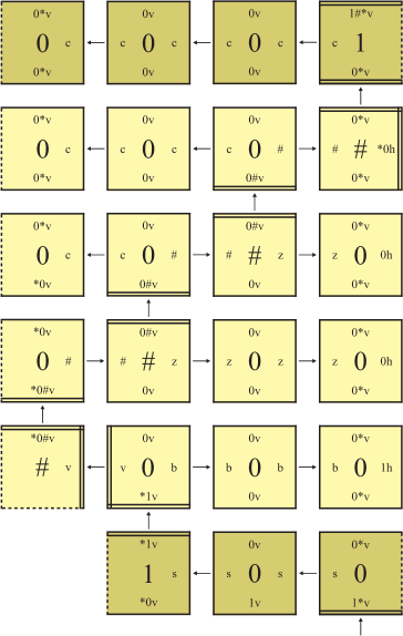
Figure 14: The self-assembly of $S_{2}^{\uparrow}$ above the topmost row of $\widetilde{Y}_{1}$.

We now have the machinery to construct a directed TAS in which $Y$ strictly self-assembles.

Lemma 5.13.

There is a $\tau$-$T$-assembly sequence $\vec{\alpha}=(\alpha_{i}|\;0\leq i<k)$, with $\alpha=\textrm{res}(\vec{\alpha})$, satisfying

1. $\alpha_{0}=\sigma$, where, for all $\vec{m}\in\mathbb{Z}^{2}$,

   $$\sigma(\vec{m})=\left\{\begin{array}[]{ll}\textmd{the tile type shown in Figure~{}15}&\textmd{if }\vec{m}=(0,1)\\ \uparrow&\textmd{otherwise,}\end{array}\right.$$

2. ${\rm dom}\;{\alpha}=Y$,

3. $\alpha$ is locally deterministic, and

4. for all $\vec{m}\in{\rm dom}\;{\alpha}$,

   $$\alpha\left(\vec{m}\right)(1,0)=\left\{\begin{array}[]{ll}\left(\textmd{*1h},2\right)&\textmd{if }\exists j\in\mathbb{N},\textmd{ and }\vec{m}=(0,\theta(2j+1))\\ \left(\textmd{*0h},2\right)&\textmd{if }\exists j\in\mathbb{N},\textmd{ and }\vec{m}=(0,\theta(2j))\\ \left(\textmd{0h},1\right)&\textmd{if }\exists j\in\mathbb{N},\textmd{ and }\\ &\quad\vec{m}\in\left(\{0\}\times\{\theta\left(j\right)-\rho\left(j\right)+1,\ldots,\theta\left(j\right)-1\}\right)\\ \left(\textmd{1h},1\right)&\textmd{if }\exists j\in\mathbb{N},\textmd{ and }\vec{m}=(0,\theta(j)-\rho(j))\\ \left(\lambda,0\right)&\textmd{otherwise}.\\ \end{array}\right.$$

Proof.

Simply combine Lemmas 5.11, and 5.12 to get a locally deterministic assembly sequence for $Y$. ∎

Figure 15: The seed tile type for the $y$-axis of $\mathbf{T}$.

Theorem 5.14.

$Y$ strictly self-assembles in the directed TAS $\mathcal{T}=(T,\sigma,\tau)$.

Proof.

Lemma 5.13 testifies to the fact that $\mathcal{T}$ is a locally deterministic TAS, and hence is directed. ∎

A straightforward “reflection” of $T$ will yield a directed TAS in which $X$ strictly self-assembles.

Corollary 5.15.

Let $h:\Sigma\rightarrow\Sigma$, where for all $a\in\Sigma$,

$$h(a)=\left\{\begin{array}[]{ll}\lambda&\textmd{if }a=\textmd{v}\\ a&\textmd{otherwise.}\end{array}\right.$$

$X$ strictly self-assembles in the directed TAS $\mathcal{T}^{\prime}=(T^{\prime},\sigma^{\prime},\tau)$, where

$$T^{\prime}=\left\{t^{\prime}\;|\textmd{ for all }(x,y)\in U_{2},t\in T,\;t^{\prime}(y,x)=\left(h(\textmd{rev}\left({\rm col}_{t}(x,y)\right))\textmd{h},{\rm str}_{t}(x,y)\right)\right\},$$

and, for all $\vec{m}\in\mathbb{Z}\times\mathbb{Z}$ and $(x,y)\in U_{2}$,

$$\sigma^{\prime}(\vec{m})(y,x)=\left\{\begin{array}[]{ll}\sigma(\vec{m})(x,y)&\textmd{if }\vec{m}=(1,0)\\ \uparrow&\textmd{otherwise.}\end{array}\right.$$

5.3 Self-Assembly of the Interior

We now turn our attention to the self-assembly of the interior of $\mathbf{T}$.

In the following lemma, we show how vertical bars attach to the $X$-axis.

Lemma 5.16.

Let $j\in\mathbb{N}$. If $\sigma\in\mathcal{A}^{\tau}_{T\cup T^{\prime}}$ satisfies

1. $\displaystyle{\rm dom}\;{\sigma}=X$, and

2. for all $\vec{m}\in\left(\{\theta(j)-\rho(j),\ldots,\theta(j)\}\times\{0\}\right)$,

   $$\sigma\left(\vec{m}\right)(0,1)=\left\{\begin{array}[]{ll}\left(\textmd{1*v},2\right)&\textmd{if }j\textmd{ is odd}\\ \left(\textmd{0*v},2\right)&\textmd{if }j\textmd{ is even, and }\vec{m}=\left(\theta(j),0\right)\\ \left(\textmd{1v},1\right)&\textmd{if }j\textmd{ is even, and }\vec{m}=\left(\theta(j)-\rho(j),0\right)\\ \left(\textmd{0v},1\right)&\textmd{otherwise},\end{array}\right.$$

then there is a $\tau$-$T\cup T^{\prime}$-assembly sequence $\vec{\alpha}=\left(\alpha_{i}\left|\;0\leq i<k<\infty\right.\right)$, with $\alpha=\textrm{res}(\vec{\alpha})$, satisfying

1. $\alpha_{0}=\sigma$,

2. ${\rm dom}\;{\alpha}=X\cup\left(\theta_{j}(X)+Y_{\rho(j)-1}\right)$,

3. for all $\vec{m}\in{\rm dom}\;{\alpha}-{\rm dom}\;{\sigma}$,

   $$\sum_{\vec{u}\in\textmd{IN}^{\vec{\alpha}}(\vec{m})}{\textmd{str}_{\alpha_{i_{\vec{\alpha}}(\vec{m})}}(\vec{m},\vec{u})}=\tau,$$

4. for all $\vec{m}\in{\rm dom}\;{\alpha}-{\rm dom}\;{\sigma}$ and all $t\in\left(T\cup T^{\prime}\right)-\{\alpha(\vec{m})\}$, $\vec{m}\not\in{\partial}^{\tau}_{t}{\left(\vec{\alpha}\setminus\vec{m}\right)}$, and

5. for all $\vec{m}\in{\rm dom}\;{\alpha}$,

   $$\alpha\left(\vec{m}\right)(1,0)=\left\{\begin{array}[]{ll}\left(\textmd{*1h},2\right)&\textmd{if }\exists j^{\prime}\in\mathbb{N},\textmd{ and }\vec{m}=(\theta(j),\theta(2j^{\prime}+1))\\ \left(\textmd{*0h},2\right)&\textmd{if }\exists j^{\prime}\in\mathbb{N},\textmd{ and }\vec{m}=(\theta(j),\theta(2j^{\prime}))\\ \left(\textmd{0h},1\right)&\textmd{if }\exists j^{\prime}\in\mathbb{N},\textmd{ and }\\ &\vec{m}\in(\{\theta(j)\}\times\\ &\quad\{\theta\left(j^{\prime}\right)-\rho\left(j^{\prime}\right)+1,\ldots,\theta\left(j^{\prime}\right)-1\})\\ \left(\textmd{1h},1\right)&\textmd{if }\exists j^{\prime}\in\mathbb{N}\textmd{ and }\vec{m}=(\theta(j),\theta(j^{\prime})-\rho(j^{\prime}))\\ \left(\lambda,0\right)&\textmd{otherwise}.\\ \end{array}\right.$$

Proof.

This follows directly from Lemma 5.10. ∎

Corollary 5.17.

Let $j,j^{\prime}\in\mathbb{N}$ with $1\leq j^{\prime}<2^{\rho(j)}$. If $\sigma\in\mathcal{A}^{\tau}_{T\cup T^{\prime}}$ satisfies

1. $X\cup\left(\theta_{j}(X)+Y_{\rho(j)-1}\right)\subseteq{\rm dom}\;{\sigma}\subseteq\mathbf{T}-\left((\theta(j),\theta(j^{\prime}))+X_{\rho\left(j^{\prime}\right)-1}\right)$,

2. for all $\vec{m}\in\left(\left(\{0\}\times\{\theta\left(j^{\prime}\right)-\rho\left(j^{\prime}\right),\ldots,\theta\left(j^{\prime}\right)\}\right)+(\theta(j),0)\right)$,

   $$\alpha\left(\vec{m}\right)(1,0)=\left\{\begin{array}[]{ll}\left(\textmd{*1h},2\right)&\textmd{if }j^{\prime}\textmd{ is odd}\\ \left(\textmd{*0h},2\right)&\textmd{if }j^{\prime}\textmd{ is even, and }\vec{m}=(\theta(j),\theta(j^{\prime}))\\ \left(\textmd{1h},1\right)&\textmd{if }j^{\prime}\textmd{ is even, and }\vec{m}=(\theta(j),\theta(j^{\prime})-\rho(j^{\prime}))\\ \left(\textmd{0h},1\right)&\textmd{otherwise,}\\ \end{array}\right.$$

there is a $\tau$-$T\cup T^{\prime}$-assembly sequence $\vec{\alpha}=(\alpha_{i}\;|\;0\leq i<k<\infty)$ satisfying

1. $\alpha_{0}=\sigma$,

2. $X\cup\left(\theta_{j}(X)+Y_{\rho(j)-1}\right)\cup\left((\theta(j),\theta(j^{\prime}))+X_{\rho\left(j^{\prime}\right)-1}\right)\subseteq{\rm dom}\;{\alpha}\subseteq{\rm dom}\;{\sigma}\cup\left((\theta(j),\theta(j^{\prime}))+X_{\rho\left(j^{\prime}\right)-1}\right)$,

3. for all $\vec{m}\in{\rm dom}\;{\alpha}-{\rm dom}\;{\sigma}$,

   $$\sum_{\vec{u}\in\textmd{IN}^{\vec{\alpha}}(\vec{m})}{\textmd{str}_{\alpha_{i_{\vec{\alpha}}(\vec{m})}}(\vec{m},\vec{u})}=\tau,$$

4. for all $\vec{m}\in{\rm dom}\;{\alpha}-{\rm dom}\;{\sigma}$ and all $t\in\left(T\cup T^{\prime}\right)-\{\alpha(\vec{m})\}$, $\vec{m}\not\in{\partial}^{\tau}_{t}{\left(\vec{\alpha}\setminus\vec{m}\right)}$, and

5. for all $\vec{m}\in{\rm dom}\;{\alpha}-{\rm dom}\;{\sigma}$,

   $$\alpha\left(\vec{m}\right)(1,0)=\left\{\begin{array}[]{ll}\left(\textmd{*1v},2\right)&\textmd{if }\exists j^{\prime\prime}\in\mathbb{N},\textmd{ and }\vec{m}=(\theta(2j^{\prime\prime}+1),\theta(j^{\prime}))\\ \left(\textmd{*0v},2\right)&\textmd{if }\exists j^{\prime\prime}\in\mathbb{N},\textmd{ and }\vec{m}=(\theta(2j^{\prime\prime}),\theta(j^{\prime}))\\ \left(\textmd{0v},1\right)&\textmd{if }\exists j^{\prime\prime}\in\mathbb{N},\textmd{ and }\\ &\vec{m}\in(\{\theta\left(j^{\prime\prime}\right)-\rho\left(j^{\prime\prime}\right)+1,\ldots,\theta\left(j^{\prime\prime}\right)-1\}\\ &\quad\times\{\theta(j^{\prime})\})\\ \left(\textmd{1v},1\right)&\textmd{if }\exists j^{\prime\prime}\in\mathbb{N},\textmd{ and }\vec{m}=(\theta(j^{\prime\prime})-\rho(j^{\prime\prime}),\theta(j^{\prime}))\\ \left(\lambda,0\right)&\textmd{otherwise}.\\ \end{array}\right.$$

Note that the results of this subsection are invariant under “reflection.”

5.4 Proof of Correctness

We are now ready to prove our second main theorem.

Lemma 5.18.

Let

$$T_{\mathbf{T}}=T\cup T^{\prime}\cup\{\textmd{the tile type shown in Figure~{}16}\}.$$

There is a $\tau$-$T_{\mathbf{T}}$-assembly sequence $\vec{\alpha}=(\alpha_{i}\;|\;0\leq i<k)$, with $\alpha=\textrm{res}(\vec{\alpha})$, satisfying

1. $\alpha_{0}=\sigma_{\mathbf{T}}$, where, for all $\vec{m}\in\mathbb{Z}\times\mathbb{Z}$,

   $$\sigma_{\mathbf{T}}(\vec{m})=\left\{\begin{array}[]{ll}\textmd{the tile type shown in Figure~{}16}&\textmd{if }\vec{m}=(0,0)\\ \uparrow&\textmd{otherwise,}\end{array}\right.$$

2. ${\rm dom}\;{\alpha}=\mathbf{T}$, and

3. $\vec{\alpha}$ is locally deterministic.

Proof.

Simply dovetail the assembly sequences given by Lemmas 5.13, 5.16, and Corollary 5.17, to get a locally deterministic assembly sequence for $\mathbf{T}$. ∎

Figure 16: The single seed tile type for $\mathbf{T}$.

Theorem 5.19.

$\mathbf{T}$ strictly self-assembles in the directed TAS $\mathcal{T}_{\mathbf{T}}=(T_{\mathbf{T}},\sigma_{\mathbf{T}},\tau)$.

Proof.

This follows immediately from Lemma 5.18. ∎

Acknowledgment

We thank Dave Doty, Xiaoyang Gu, Satya Nandakumar, John Mayfield, Matt Patitz, Aaron Sterling, and Kirk Sykora for useful discussions.

References

- [1] L. Adleman, Towards a mathematical theory of self-assembly, Tech. report, University of Southern California, 2000.
- [2] Leonard M. Adleman, Qi Cheng, Ashish Goel, Ming-Deh A. Huang, David Kempe, Pablo Moisset de Espanés, and Paul W. K. Rothemund, Combinatorial optimization problems in self-assembly, Proceedings of the Thirty-Fourth Annual ACM Symposium on Theory of Computing, 2002, pp. 23–32.
- [3] Leonard M. Adleman, Jarkko Kari, Lila Kari, and Dustin Reishus, On the decidability of self-assembly of infinite ribbons, Proceedings of the 43rd Annual IEEE Symposium on Foundations of Computer Science, 2002, pp. 530–537.
- [4] T. M. Apostol, Modular functions and Dirichlet series in number theory, Graduate Texts in Mathematics, vol. 41, Springer-Verlag, 1997.
- [5] Qi Cheng, Ashish Goel, and Pablo Moisset de Espanés, Optimal self-assembly of counters at temperature two, Proceedings of the First Conference on Foundations of Nanoscience: Self-assembled Architectures and Devices, 2004.
- [6] D. Doty, X. Gu, J.H. Lutz, E. Mayordomo, and P. Moser, Zeta-Dimension, Proceedings of the Thirtieth International Symposium on Mathematical Foundations of Computer Science, Springer-Verlag, 2005, pp. 283–294.
- [7] L. Euler, Variae observationes circa series infinitas, Commentarii Academiae Scientiarum Imperialis Petropolitanae 9 (1737), 160–188.
- [8] K. Falconer, Fractal geometry: Mathematical foundations and applications, second ed., Wiley, 2003.
- [9] Ronald L. Graham, Donald E. Knuth, and Oren Patashnik, Concrete mathematics, Addison-Wesley, 1994.
- [10] G. Hardy and E. Wright, An introduction to the theory of numbers, 5th ed., Clarendon Press, 1979.
- [11] John H. Reif, Molecular assembly and computation: From theory to experimental demonstrations, Proceedings of the Twenty-Ninth International Colloquium on Automata, Languages and Programming, 2002, pp. 1–21.
- [12] Paul W. K. Rothemund, Theory and experiments in algorithmic self-assembly, Ph.D. thesis, University of Southern California, December 2001.
- [13] Paul W. K. Rothemund and Erik Winfree, The program-size complexity of self-assembled squares (extended abstract)., Proceedings of the Thirty-Second Annual ACM Symposium on Theory of Computing, 2000, pp. 459–468.
- [14] Paul W.K. Rothemund, Nick Papadakis, and Erik Winfree, Algorithmic self-assembly of DNA Sierpinski triangles, PLoS Biology 2 (2004), no. 12.
- [15] N.C. Seeman, Nucleic-acid junctions and lattices, Journal of Theoretical Biology 99 (1982), 237–247.
- [16] David Soloveichik and Erik Winfree, Complexity of self-assembled shapes, SIAM Journal on Computing 36, 2007, pp. 1544–1569.
- [17] Hao Wang, Proving theorems by pattern recognition – II, The Bell System Technical Journal XL (1961), no. 1, 1–41.
- [18] , Dominoes and the AEA case of the decision problem, Proceedings of the Symposium on Mathematical Theory of Automata (New York, 1962), Polytechnic Press of Polytechnic Inst. of Brooklyn, Brooklyn, N.Y., 1963, pp. 23–55.
- [19] S. J. Willson, Growth rates and fractional dimensions in cellular automata, Physica D 10 (1984), 69–74.
- [20] Erik Winfree, Algorithmic self-assembly of DNA, Ph.D. thesis, California Institute of Technology, June 1998.