Corrugated waveguide under scaling investigation

Abstract

Some scaling properties for classical light ray dynamics inside a periodically corrugated waveguide are studied by use of a simplified two-dimensional nonlinear area-preserving map. It is shown that the phase space is mixed. The chaotic sea is characterized using scaling arguments revealing critical exponents connected by an analytic relationship. The formalism is widely applicable to systems with mixed phase space, and especially in studies of the transition from integrability to non-integrability, including that in classical billiard problems.

Interest in the problem of guiding a light ray inside a periodically corrugated boundary has increased in recent years, partly because the topic is applicable in so many different fields of science. Applications involve e.g. ray chaos in underwater acoustics ref1 ; ref2 ; ref3 , scattering of a quantum particle in a rippled waveguide ref4 , quantized ballistic conductance in a periodically modulated quantum channel ref5 , quantum transport in ballistic cavities ref6 , transport through a finite ${\rm GaAs/Al_{x}Ga_{1-x}As}$ heterostructure ref8 , comparisons of classical v. quantum behavior in periodic mesoscopic systems ref9 , and anomalous wave transmittance in the stop band of a corrugated parallel-plane waveguide ref11 .

There are many different ways of describing problems involving waveguides. One of them is the well known billiard description, and such a procedure is used in the present paper. A billiard problem consists of a system in which a point particle moves freely inside a bounded region and suffers specular reflections with the boundaries. Generally, the dynamics is described using the formalism of discrete maps. Depending on the combinations of control parameter values, as well as on the initial conditions, the phase spaces for such mappings fall into three distinct classes, namely: (i) regular; (ii) ergodic; or (iii) mixed. Generally, the integrability of the regular cases is related to angular momentum conservation, the static circular billiard being a typical example. On the other hand, for completely ergodic billiards, only chaotic and unstable periodic orbits are present in the dynamics. Two examples of case (ii) are the Bunimovich stadium ref12 and the Sinai billiard ref14 . For these two systems, the time evolution of a single initial condition, for the appropriate combinations of control parameters, is enough to fill the whole phase space, ergodically. Finally, there are many billiards of mixed phase space structure ref15 ; ref17 ; ref18 ; ref19 ; add1 ; add3 , having a range of control parameters whose physical significances differ. Depending on the combination of both initial conditions and control parameters, the phase space presents a very rich structure containing invariant spanning curves (sometimes known as invariant tori), Kolmogorov-Arnold-Moser (KAM) islands, and chaotic seas.

In this Letter, I use scaling arguments to describe the behavior of the variance of the average reflection angle, within the chaotic sea, for a classical light ray undergoing specular reflections inside a periodically corrugated waveguide. The model consists of a classical light ray that is specularly reflected between a corrugated surface given by $y=y_{0}+d\cos(kx)$ and a flat plane surface at $y=0$. The term $y_{0}$ denotes the average distance between the corrugated and flat surfaces, $d$ is the amplitude of the corrugation and $k$ is the wave number. The dynamical variables used in the description of the problem are the angle $\theta$ of the ray’s trajectory measured from the positive horizontal axis, and the corresponding value of the $x$ coordinate at the instant of reflection. Moreover, the mapping is iterated when the light hits the surface $y=0$; thus multiple reflections with the corrugated surface can be neglected.

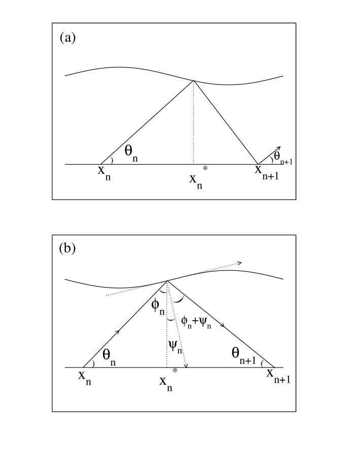
Figure 1: (a) Reflection from the corrugated surface of a light ray coming from the flat surface at $y=0$. (b) Details of the trajectory before and after a collision with the corrugated surface.

The problem lies in obtaining the map $T(x_{n},\theta_{n})=(x_{n+1},\theta_{n+1})$, given the initial conditions $(x_{n},\theta_{n})$ shown in Fig. 1(a). From the geometrical considerations illustrated in the figure, it is easy to see that $x_{n}^{*}-x_{n}=(y_{0}+d\cos(kx_{n}^{*}))/\theta_{n}$, and similarly that

$$x_{n+1}-x_{n}^{*}=(y_{0}+d\cos(kx_{n}^{*}))/\theta_{n+1}~{}.$$ (1)

The term $x_{n}^{*}$ gives the location of the collision on the corrugated surface. The angle $\theta_{n}$ is written as

$$\theta_{n+1}=\theta_{n}-2\psi_{n}~{},$$ (2)

where $\tan(\psi_{n}(x))=dy(x)/dx=-dk\sin(kx_{n}^{*})$ gives the slope of the surface at $x=x_{n}^{*}$. Equations (1) and (2) correspond to the exact mapping. However in this paper we make the following approximations: (a) we assume that $d/y_{0}\ll 1$, so that $y_{0}+d\cos(kx_{n}^{*})\cong y_{0}$; (b) in the same limit, we also assume that $\tan(\psi_{n})\cong\psi_{n}$. The condition $d/y_{0}\ll 1$ holds in practice for studies of wave propagation in a corrugated waveguide ref3 . It also applies to the investigation of transport in mesoscopic channels ref9 and can even be used in the characterization of wave propagation in deep ocean ref1 ; ref2 . In the description of the mapping, it is convenient to use dimensionless variables, $\delta=d/y_{0}$, $\gamma_{n}=\theta_{n}/k$ and $X_{n}=kx_{n}/y_{0}$. Thus, the simplified two-dimensional nonlinear mapping is given by

$$T:\left\{\begin{array}[]{ll}X_{n+1}=X_{n}+\left[{{1}\over{\gamma_{n}}}+{{1}\over{\gamma_{n+1}}}\right]~{}~{}{\rm mod(2\pi)}\\ \gamma_{n+1}=\gamma_{n}+2\delta\sin\left(X_{n}+{{1}\over{\gamma_{n}}}\right){}{}\\ \end{array}\right.~{}.$$ (3)

The determinant of the Jacobian matrix for this mapping is unity, so that it is area-preserving. The mapping (3) is described by a single effective control parameter, $\delta$. If $\delta=0$, the system is integrable while for $\delta\neq 0$, the phase space is mixed, containing both chaos and regularity (fixed points and quasiperiodic behavior). The system thus experiences an abrupt transition from integrability to non-integrability when going from $\delta=0$ to $\delta\neq 0$. I shall investigate some dynamical properties for very small values of $\delta$ (which meets the initial approximation $d/y_{0}\ll 1$) near the transition, using scaling arguments. There is a wide range of systems exhibiting transitions from integrability to non-integrability, and the formalism used in the present model can be in principle be extended to them, in particular to identify classes of universality.

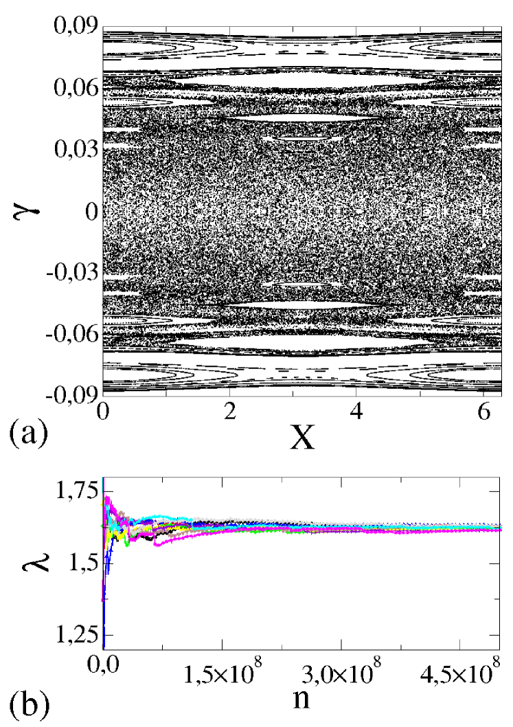
Figure 2: (Color online) (a) Phase space for the mapping (3) with the control parameter $\delta=10^{-3}$. (b) Positive Lyapunov exponent obtained via the triangularization algorithm.

Fig. 2(a) shows the phase space generated by iterating the map (3) for the control parameter $\delta=10^{-3}$. It is easy to see that the phase space is of mixed form, including invariant spanning curves, KAM islands and a large chaotic sea for both positive and negative values of the variable $\gamma$. The invariant spanning curves limit the size of the chaotic sea and correspondingly yield a limited range of possible values for the chaotic orbits. Fig. 2(b) shows positive Lyapunov exponents obtained for the chaotic sea using the triangularization algorithm ref24 , for the control parameter $\delta=10^{-3}$. An ensemble of $10$ different initial conditions was iterated $5\times 10^{8}$ times. The initial conditions considered were $X_{0}=\delta$ and 10 different values of $\gamma_{0}$ uniformly distributed in the interval $\gamma\in[0,2\pi)$. The average value obtained was ${\bar{\lambda}}=1.624(7)$, where 0.007 is the standard deviation obtained from the 10 samples.

The existence of invariant spanning curves limiting the size of the chaotic sea confers an interesting property on the chaotic orbits. From an initial condition in the region of the chaotic sea, the system wanders within the entire accessible region but it is always confined between two invariant spanning curves. The location of the first positive and negative invariant spanning curves depends on the value of the control parameter. As a consequence, the “amplitude” of a chaotic time series is also dependent on the control parameter, so that the average value tends only gradually towards a regime of convergence. With this property in mind, I now explore the behavior of the deviation of the average value for the angle $\gamma$, or roughness, an observable defined as

$$\omega(n,\delta)={{1}\over{M}}\sum_{i=1}^{M}\sqrt{\bar{\gamma_{i}^{2}}(n,\delta)-{\bar{\gamma_{i}}}^{2}(n,\delta)}~{},$$ (4)

where

$$\bar{\gamma}(n,\delta)={{1}\over{n}}\sum_{i=0}^{n}\gamma_{i}~{}.$$ (5)

Equation (4) was iterated using an ensemble of $M=5\times 10^{3}$ different initial conditions. The variable $\gamma_{0}$ was kept fixed at $\gamma_{0}=10^{-2}\delta$ while the $5000$ values of $X_{0}$ were uniformely distributed along $X_{0}\in[0,2\pi)$. Fig. 3(a) shows the behavior of three different values of the roughness for different control parameters.

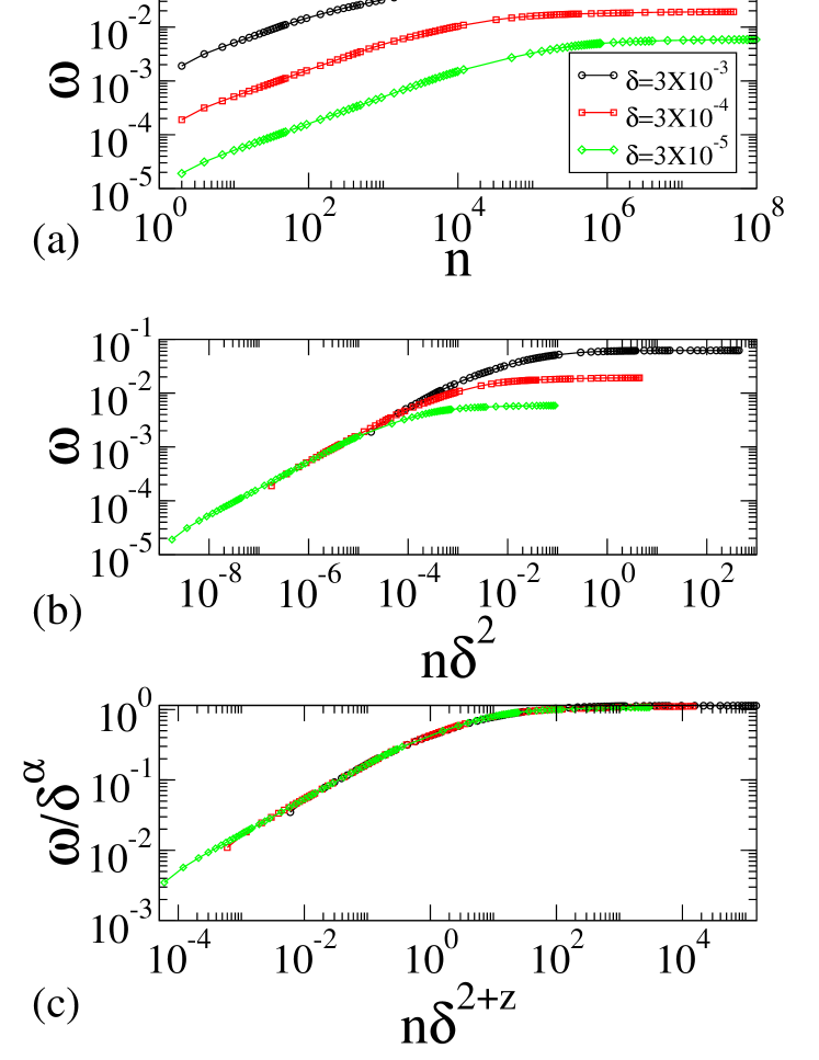
Figure 3: (Color online) (a) Roughness $\omega$ as a function of the iteration number $n$ for three different control parameters. (b) After a suitable change of variables, all three curves start by growing together. (c) Their collapse onto a single universal plot.

One can observe that, as the number of iterations increases, the roughness grows at first, but then suddenly bends over towards a regime of saturation. The

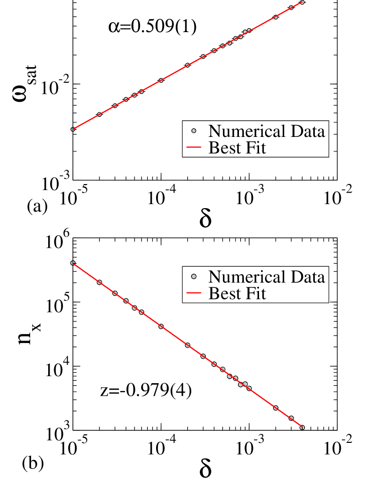
Figure 4: (Color online) Plots of (a) $\omega_{\rm sat}$ and (b) the crossover iteration number $n_{x}$ as function of the control parameter $\delta$.

changeover from growth to saturation is marked by a characteristic crossover iteration number denoted as $n_{x}$. Note that different values of the control parameter generate different roughness curves for small iteration numbers $n$. Applying the transformation $n\rightarrow n\delta^{2}$ yields a coalescence of all the curves at small iteration number, as can be seen in Fig. 3(b). Based on the behavior of Fig. 3(a), the following three scaling hypotheses are proposed: (i) that for small iteration numbers, say $n\ll n_{x}$, the roughness behaves according to the power law

$$\omega(n\delta^{2},\delta)\propto(n\delta^{2})^{\beta}~{},$$ (6)

where we refer to the critical exponent $\beta$ as the growth exponent; (ii) for large enough iteration number, $n\gg n_{x}$, the roughness approaches a regime of saturation marked by a constant “plateau” given by

$$\omega_{\rm sat}\propto\delta^{\alpha}~{},$$ (7)

where we call the exponent $\alpha$ the roughening exponent; finally (iii) the number of iterations that characterizes the crossover, i.e. that marks the change from growth to saturation is written as

$$n_{x}\propto\delta^{z}~{}.$$ (8)

The exponent $z$ is a dynamical exponent. These three scaling hypothesis are extensions of the formalism used in surface science (see e.g. Ref. add2 ). Based on these three initial suppositions, the roughness can now be described in terms of a scaling function of the type

$$\omega(n\delta^{2},\delta)=l\omega(l^{a}n\delta^{2},l^{b}\delta)~{},$$ (9)

where $l$ is a scaling factor, and $a$ and $b$ are scaling exponents. Moreover, the exponents $a$ and $b$ must be related to the critical exponents $\alpha$, $\beta$ and $z$. Because $l$ is a scaling factor, we can specify that $l=(n\delta^{2})^{(-1/a)}$ and rewrite Eq. (9) as

$$\omega(n\delta^{2})=(n\delta^{2})^{(-1/a)}\omega_{1}([n\delta^{2}]^{(-b/a)}\delta)~{},$$ (10)

where the function $\omega_{1}=\omega(1,[n\delta^{2}]^{-b/a}\delta)$ is assumed to be constant in the limit of $n\ll n_{x}$. Comparison of Eqs. (10) and (6) allows one to conclude immediately that $\beta=-1/a$. Choosing now that $l=\delta^{-1/b}$, Eq. (9) is given by

$$\omega(n\delta^{2},\delta)=\delta^{-1/b}\omega_{2}(\delta^{-(a/b)}n\delta^{2})~{},$$ (11)

where the function $\omega_{2}=\omega(\delta^{-(a/b)}n\delta^{2},1)$ is supposed constant for $n\gg n_{x}$. Comparing Eqs. (11) and (7), we find that $\alpha=-1/b$. Given the two different expressions for the scaling factor $l$, one must conclude that the relation between the critical exponents takes the form

$$z={{\alpha}\over{\beta}}-2~{}.$$ (12)

Note that the scaling exponents are all determined if the critical exponents $\alpha$ and $\beta$ can be obtained numerically. Fig. 4(a) and (b) show the behavior of $\omega_{\rm sat}$ and $n_{x}$ respectively as functions of $\delta$. The saturation values were obtained by extrapolation because, even after almost $10^{3}n_{x}$ iterations, the roughness is still not approaching its saturation value. Fitting a power law to the results of Figs. 4(a) and (b), it was found that $\alpha=0.509(1)$, $\beta=0.4997(8)$ and $z=-0.979(4)$. The dynamical exponent $z$ can also be obtained from Eq. (12), by evaluation of the numerical values of $\alpha$ and $\beta$, yielding $z=-0.9814(3)$. This result is in excellent agreement with the numerical result obtained in Fig. 4(b).

With the values of the critical exponents now obtained, the scaling hypotheses can be verified. Fig. 3(c) illustrates the collapse of the three different roughness curves generated from different values of the control parameter onto a single universal roughness plot. Such a collapse confirms that the scaling suppositions are indeed correct despite the three decades used in the control parameter $\delta$. In the construction of all the roughness curves, the value of the dynamical variable $\gamma_{0}$ was set at $\gamma_{0}=10^{-2}\delta$. If one increases the initial value of $\gamma_{0}$, the scaling hypotheses will remain valid, but an extra scaling time (say $n_{x}^{\prime}$) appears. Even considering the new extra crossover iteration number, scaling exponents can still be obtained ref22 .

In summary, the problem of light ray reflection in a periodically corrugated waveguide has been addressed. The chaotic sea confined between the first two invariant spanning curves (the positive and negative ones) was characterized using scaling arguments. In particular, the deviation of the average value of $\gamma$ was obtained as functions of both the control parameter $\delta$ and the iteration number $n$. Three scaling hypotheses were proposed, and then confirmed by the perfect collapse of all curves onto a single universal plot, confirming that the system experiences a transition from integrability to non-integrability. Finally, the obtained critical exponents $\alpha$, $\beta$ and $z$ allow us to conclude that the present corrugated waveguide model belongs to the same class of universality of the one-dimensional bouncing ball model.

E.D.L. thanks Prof. J. K. L. da Silva and Prof. P.V.E. McClintock for helpful discussions. Support from CNPq, FAPESP and FUNDUNESP, Brazilian agencies is gratefully acknowledged.

References

- (1) A. L. Virovlyansky and G. M. Zaslavsky, Chaos 10, 211 (2000).
- (2) I. P. Smirnov, A. L. Virovlyansky and G. M. Zaslavsky, Phys. Rev. E 64, 036221, (2001).
- (3) A. Iomin, Yu. Bliokh, Comm. Non. Sci. and Num. Simul. 8, 389, (2003).
- (4) G. B. Akguc and L. E. Reichl, Phys. Rev. E 67, 046202, (2003).
- (5) M. Leng and C. S. Lent, Phys. Rev. Lett. 71, 137, (1993).
- (6) B. Huckestein, R. Ketzmerick and C. H. Lewenkopf, Phys. Rev. Lett. 84, 5504, (2000); Phys. Rev. Lett. 87, 119901, (2001).
- (7) L. P. Kouwenhoven, F. W. J. Hekking, B. J. van Wees, C. J. P. M. Harmans, C. E. Timmering and C. T. Foxon, Phys. Rev. Lett. 65, 361, (1990).
- (8) G. A. Luna-Acosta, J. A. Méndez-Bermúdez and F. M. Izrailev, Phys. Rev. E 64, 036206, (2001); Phys. Lett. A 274, 192, (2000).
- (9) R. B. Hwang, IEEE Tran. Ant. and Prop. 54, 755, (2006).
- (10) L. A. Bunimovich, Math. USSR Sb. 23, 45, (1974); Commun. Math. Phys. 65, 295, (1979).
- (11) Y. G. Sinai, Russian Math. Surveys 25, 137, (1970).
- (12) M. V. Berry, Eur. J. Phys. 2, 91, (1981). 12, 1363, (1999).
- (13) M. Robnik, J. Phys. A: Math. Gen. 16, 3971, (1983).
- (14) M. Robnik and M. V. Berry, J. Phys. A: Math. Gen. 18, 1361, (1985).
- (15) R. Markarian, S. O. Kamphorst and S. P. de Carvalho, Commun. Math. Phys. 174, 661, (1996).
- (16) R. Egydio de Carvalho, Phys. Rev. E 55, 3781 (1997).
- (17) E. D. Leonel and P. V. E. McClintock, J. Phys. A 38, 823, (2005); Chaos 15, 033701, (2005).
- (18) J.-P. Eckmann and D. Ruelle, Rev. Mod. Phys. 57, 617, (1985).
- (19) A. -L. Barabási, H. E. Stanley, Fractal Concepts in Surface Growth (Cambridge University Press, Cambridge, 1995).
- (20) E. D. Leonel, P. V. E. McClintock and J. K. L. da Silva, Phys. Rev. Lett. 93, 014101 (2004).