Decay of Correlations for Sparse Graph Error Correcting Codes

Abstract

The subject of this paper is transmission over a general class of binary-input memoryless symmetric channels using error correcting codes based on sparse graphs, namely low-density generator-matrix and low-density parity-check codes. The optimal (or ideal) decoder based on the posterior measure over the code bits, and its relationship to the sub-optimal belief propagation decoder, are investigated. We consider the correlation (or covariance) between two codebits, averaged over the noise realizations, as a function of the graph distance, for the optimal decoder. Our main result is that this correlation decays exponentially fast for fixed general low-density generator-matrix codes and high enough noise parameter, and also for fixed general low-density parity-check codes and low enough noise parameter. This has many consequences. Appropriate performance curves - called GEXIT functions - of the belief propagation and optimal decoders match in high/low noise regimes. This means that in high/low noise regimes the performance curves of the optimal decoder can be computed by density evolution. Another interpretation is that the replica predictions of spin-glass theory are exact. Our methods are rather general and use cluster expansions first developed in the context of mathematical statistical mechanics.

1 Introduction

Low-density parity-check (LDPC) codes based on sparse graphs have emerged as a focal point in the theory of error correcting codes, used in noisy channel communication, largely because they are amenable to low complexity decoding and at the same time have a good performance (measured as the gap to Shannon’s capacity). An important class of low complexity decoders are the message passing iterative decoders. In this framework, in order to decode a bit attached to a node of the graph, one unravels a computational tree (or covering tree) and iteratively updates messages (suitable functions of the channel output observations) passed along the edges of the computational tree. We refer to the recent book [1] for the state of the art of this general theory. One would also like to be able to compare sub-optimal message passing decoders with the optimal or ideal decoder. The later is based on the posterior probability distribution supported on code-bits and is optimal in the sense that it is known to minimize the bit-error-rate among all decoders (it is also called MAP decoder, and this is the terminology that we adopt in this paper). A priori the comparison of decoders is not easily done since the MAP decoder is in general computationaly complex.

One of the most important low complexity message passing decoders is the belief propagation (BP) algorithm. It is well known that for a code whose graph is a tree, the BP algorithm has the same performance as the MAP decoder. This essentially comes from the fact that on a tree the computational graph of a node matches the original graph itself. However, codes based on tree graphs have poor performance and one needs to consider graphs with loops or cycles. With cycles in the original graph, the messages on the computational tree are no longer independent, and it is not a priori clear, if and why, the BP algorithm should retain any close relationship to the MAP decoder. A fundamental theoretical tool that allows to analyze the BP algorithm is density evolution (DE) first developed in [2]. From DE one can for example obtain a noise threshold above which reliable communication is not possible with BP decoding. The analysis proceeds by taking first a very large block length $n$ and looking at $d\ll n$ iterations of the BP decoder. Eventualy one considers the asymptotics $\lim_{d\to+\infty}\lim_{n\to+\infty}$. However, in the practical use of the decoder one fixes $n$ (large) and the iterations $d\gg n$ are performed till one reaches an acceptably small bit-error-rate. This corresponds to the asymptotics $\lim_{n\to+\infty}\limsup/{\rm inf}_{d\to+\infty}$. The practical success of density evolution relies on the equivalence of these two limiting procedures, an open problem in general.

It is fair to say that these issues have been resolved over the binary erasure channel (BEC) [1] (the analysis however has not proceeded from the point of view of the correlations of the MAP decoder). An important tool in the analysis over the BEC has been the ”extended BP“ extrinsic information transfer (EXIT) curve (which is a suitable continuation of the bit-error-rate curve under BP decoding). Recently it was shown that the bit-error-rate of the MAP decoder can be obtained from that of the extended BP EXIT curve by a Maxwell construction just as in the theory of first order phase transitions [6], [7]. This construction allows to compute the MAP noise threshold, and to compare it to the BP noise threshold. The validity of the exchange of limits $d\to+\infty$ and $n\to+\infty$ (for the BP decoder) can also be derived for the BEC using natural monotonicity properties of the decoder [1].

For the case of transmission over more general channels very little is known about these issues. Indeed there one lacks the combinatorial methods available for the BEC, and radically new methods have to be used. Convenient measures of the performance, which generalize the EXIT curves, are the so-called GEXIT curves [1] (see the next section for their precise definition). It is believed that in terms of these, the results obtained for the BEC still hold. In particular, the GEXIT curves for the BP and the MAP decoder should match for high and low noise regimes away from the phase transition thresholds. Such conjectures are supported by spin glass theory calculations (e.g the replica and cavity methods) which provide conjectural but analytic formulas. One-sided bounds have been derived for the GEXIT curves by the (information theoretical) method of physical degradation [1] and also by using correlation inequalities valid for spin glasses [13]. Related bounds on the conditional input-output entropy have also been derived [3], [4] by using ”interpolation methods” first developed in the mathematical theory of spin glasses [5], [8], [9]. As it turns out, all these bounds match the replica expressions and are therefore believed to be the best possible. In [10] the interpolation method has been extended to obtain the converse bounds for a class of Poissonian LDPC codes over the BEC, thus recovering combinatorial results of [11] in a completely different way. Concerning the problem of exchanging the $d,n\to+\infty$ limits we refer to [15] for recent progress that goes beyond the BEC.

In this work we will show that a good deal can be learned by looking at the correlations (more precisely the covariance), averaged over the channel outputs, of the MAP decoder. We comment below about the methods used, but let us say at the outset that our aim is to cover a fairly general class of binary input memoryless symmetric channels, including the binary symmetric and gaussian ones. One of our main results is that for sufficiently low noise (LDPC codes) the correlations between two code-bits decay exponentially fast as a function of the graph distance between the two code-bits, uniformly in the block length size $n$. The sparsity of the underlying graph then implies that, if furthermore the decay rate beats the local expansion of the graph, the MAP GEXIT curve can be computed by DE. Another interpretation of this result is that the solutions provided by the replica/cavity methods of spin glass theory are exact.

Low-density generator-matrix codes (LDGM) codes have a very clear relationship to spin glass models on random graphs and it is useful to study them before we can attack the harder case of LDPC codes. Besides, the present analysis could potentially be useful in other contexts where they are used (e.g. rateless codes, source coding). For high noise we prove the decay of correlations and that the MAP GEXIT curve can be computed by DE. For that system, we can also show that the decay of correlations implies that the limits $d,n\to+\infty$ can be exchanged for the BP decoder, at least on the binary symmetric channel.

The study of the behavior of correlations as a function of the distance between local degrees of freedom is one of the central aims of statistical physics. For lattice spin systems (e.g. the Ising model) an important criterion that ensures correlation decay is Dobrushin’s criterion [12] - which is of probabilistic nature - and its various improvements. The main other method - which is not necessarily of probabilistic nature - is based on suitable expansions in powers of “the strength of interactions”. There exists a host of such expansions collectively called “cluster expansions”, and the context of spin systems the first and simplest such expansion is the so-called “polymer expansion” [16]. The main rule of thumb is that all these methods work if the degrees of freedom are weakly interacting, or if one can transform the original system into an effective one involving new weakly interacting degrees of freedom. It turns out that sophisticated forms of the cluster expansions can be carried out, for LDGM codes in a high noise regime, and for LDPC codes in a low noise regime, for a fairly general class of channels including the binary symmetric channel (BSC) as well as the binary input additive white gaussian noise channel (BIAWGNC). As we will explain later it is necessary to use quite sophisticated cluster expansions for at least two reasons. Concerning LDGM codes Dobrushin’s criterion and the polymer expansion require bounded channel outputs (and thus do not covers the case of the BIAWGNC). Concerning LDPC codes one has to transform the system to a dual one that involves ”negative Gibbs weights” and cannot even be treated by probabilistic methods.

The rest of the paper is organized as follows. In section 2 we formulate the models and give a unified view of the main results both for LDGM and LDPC codes. The main strategy of the proofs is also explained there. Sections 3 and 4 contain the proofs of correlation decay and its consequences for the GEXIT curves. The problem of exchanging the limits of iteration number and block length size is addressed in section 5. We conclude by pointing out open problems and further connections to the recent literature. The appendix reviews in a streamlined form the two cluster expansions that are used in sections 3 and 4.

Summaries of the present results have been reported for the special case of the BIAWGNC [17], [18].

2 Models and Main Results

We consider binary-input memoryless output-symmetric channels defined by a transition p.d.f $p_{Y\mid X}(y\mid x)$ with inputs $x\in\{-1,+1\}$ and outputs belonging to $\mathbb{R}$. Since we use techniques from statistical mechanics it is convenient to immediately map the usual input alphabet $\{0,1\}$ to $\{-1,+1\}$. Symmetry of the channel means that $p_{Y\mid X}(-y\mid-x)=p_{Y\mid X}(y\mid x)$. The intensity of the noise is called $\epsilon$. It will be convenient to trade off the channel outputs $y$ for the half-loglikelihood

$$l=\frac{1}{2}\ln\biggl{[}\frac{p_{Y|X}(y|+1)}{p_{Y|X}(y|-1)}\biggr{]}$$ (1)

It is well known that on a symmetric channel one can assume without loss of generality that the all-one codeword (i.e the usual all-zero codeword) is transmitted and therefore the channel outputs are i.i.d with distribution $p_{Y\mid X}(y|+1)dy\equiv c(l)dl$. For clarity, we assume that the noise parameter varies in an interval $[0,\epsilon_{max}]$ ($\epsilon_{max}$ is possibly infinite) where $\epsilon\to 0$ corresponds to low noise and $\epsilon\to\epsilon_{max}$ corresponds to high noise. For example, $\epsilon_{max}=\frac{1}{2}$ for the BSC, $\epsilon_{max}=+\infty$ for the BIAWGNC (and $\epsilon_{max}=1$ for the BEC). The general class of channels for which our main results hold is

Class of channels. We define the class $\mathcal{K}$ of binary-input memoryless output-symmetric channels:

1. The numbers $T_{2p}(\epsilon)=\frac{d}{d\epsilon}\int_{-\infty}^{\infty}dl\,c(l)(\tanh l)^{2p}$ are bounded uniformly with respect to $p\geq 1$ integer.

2. For any finite $m>0$ we have $\mathbb{E}[e^{m|l|}]\leq c_{m}<+\infty$

3. (Low noise condition) There exists $s_{0}>0$ small enough such that for $0<s\leq s_{0}$ we have $\lim_{\epsilon\to 0}\mathbb{E}[e^{-sl}]=0$.

4. (High noise condition) Set $\delta(\epsilon,H)=e^{4H}-1+\mathbb{P}(|l|>H)$. One can find $H(\epsilon)$ such that $\lim_{\epsilon\to\epsilon_{max}}\delta(\epsilon,H(\epsilon))=0$.

Note that this class is not the most general that we can treat but it is at the same time fairly general and keeps the analysis at a technically reasonable level. An important example is the BSC (we keep $0\leq\epsilon\leq\frac{1}{2})$

$$p_{Y|X}(y|x) =(1-\epsilon)\delta(y-x)+\epsilon\delta(y+x),$$

$$c(l) =(1-\epsilon)\delta(l-\frac{1}{2}\ln\frac{1-\epsilon}{\epsilon})+\epsilon\delta((l-\frac{1}{2}\ln\frac{\epsilon}{1-\epsilon})$$ (2)

One can check that the conditions are met with $T_{2p}(\epsilon)=2p(1-2\epsilon)^{2p-1}$, $\mathbb{E}[e^{m|l|}]=(\frac{1-\epsilon}{\epsilon})^{\frac{m}{2}}$, $\mathbb{E}[e^{-sl}]=\epsilon^{\frac{s}{2}}(1-\epsilon)^{1-\frac{s}{2}}+(1-\epsilon)^{\frac{s}{2}}\epsilon^{1-\frac{s}{2}}$ and $H(\epsilon)=\log\frac{1-\epsilon}{\epsilon}$. Another important example is the BIAWGNC

$$p_{Y|X}(y|x)=\frac{1}{\sqrt{2\pi}\epsilon}\exp\biggl{(}-\frac{(y-x)^{2}}{2\epsilon}\biggr{)},\,\,c(l)={\frac{\epsilon}{\sqrt{2\pi}}}\exp\biggl{(}-\frac{(l-\epsilon^{-1})^{2}}{2\epsilon^{-1}}\biggr{)}$$ (3)

Again one can check that the conditions are met with $T_{2p}(\epsilon)\leq\int_{-\infty}^{+\infty}dl\,|\frac{dc(l)}{d\epsilon}|$, $\mathbb{E}[e^{m|l|}]<\infty$, $\mathbb{E}[e^{-sl}]=e^{-s\epsilon^{-1}(1-\frac{s}{2})}$ and $H(\epsilon)=2\epsilon^{-1/4}$. Note that the BEC is not contained in the class $\mathcal{K}$ because of the second condition. Nevertheless due to the special nature of this channel our methods can easily be adapted, but we will not give the details here since this is a case that has already been thoroughly analyzed in the literature [1].

Fixed LDGM codes are constructed from a fixed bipartite graph with $m$ information-bit nodes (variable nodes) and $n$ code-bit nodes (check nodes), and edges connecting variable and check nodes only. The design rate of the code $R=\frac{m}{n}$ is kept fixed. The set of neighbors of a variable node $a$ is called $\partial a$ and the set of neighbors of a check node $i$ is called $\partial i$. We consider graphs with bounded node degrees $|\partial a|\leq l_{\max}$ and $|\partial i|\leq k_{\max}$. Information bits $u_{1},...,u_{m}\in\{-1,+1\}^{m}$ are attached to the variable nodes and the code-bits $x_{1},...,x_{n}$ attached to the check nodes are obtained as

$$x_{i}=\prod_{a\in\partial i}u_{a},\qquad i=1,...,n$$ (4)

We also consider ensembles of such codes defined by random graph constructions. We do not explain the details of these constructions here except for saying that an LDGM($\Lambda,P$) ensemble is specified by the generating functions of variable (resp. check) node degree distributions $\Lambda(z)=\sum_{l=1}^{l_{\max}}\Lambda_{l}z^{l}$ (resp. $P(z)=\sum_{r=1}^{r_{\max}}P_{r}z^{r}$) [1].

Fixed LDPC codes are similarly constructed from a fixed bipartite graph with $n$ variable nodes $i=1,...,n$ (this time these are the code-bit nodes) and $m$ check nodes $c=1,...m$, with edges connecting variable and check nodes only. The design rate is $R=1-\frac{m}{n}$ is fixed. We assume that the node degrees are bounded $|\partial i|\leq l_{\max}$ and $|\partial c|\leq k_{\max}$. The code-bits $x_{1},...,x_{n}$ attached to the variable nodes satisfy $m$ parity check constraints

$$\prod_{i\in\partial c}x_{i}=1,\qquad c=1,...,m$$ (5)

We also consider ensembles of such codes defined by random graph constructions; an ensemble is specified by the generating functions of variable (resp. check) node degree distribution $\Lambda(z)=\sum_{l=1}^{l_{\max}}\Lambda_{l}z^{l}$ (resp. $P(z)=\sum_{r=1}^{r_{\max}}P_{r}z^{r}$) [1].

The optimal MAP decoder is based on the posterior measure of the transmitted codeword given the received message $y^{n}=(y_{1},..,y_{n})$. For LDGM codes this conditional measure is best viewed as being supported on information bits,

$$p_{U^{m}|Y^{n}}(u^{m}|y^{n})=\frac{1}{Z}\prod_{i=1}^{n}e^{l_{i}\prod_{a\in\partial i}u_{a}}$$ (6)

For LDPC codes the conditional measure is

$$p_{X^{n}|Y^{n}}(x^{n}|y^{n})=\frac{1}{Z}\prod_{c=1}^{m}\frac{1}{2}(1+\prod_{i\in\partial c}x_{i})\prod_{i=1}^{n}e^{l_{i}x_{i}}$$ (7)

In both cases $Z$ is the appropriate normalization factor. These measures are random because of the channel outputs and possibly because the code is chosen at random from an ensemble. The average with respect to the channel outputs is often denoted by $\mathbb{E}_{l^{n}}$ and the average with respect to a code ensemble is generically denoted by $\mathbb{E}_{\mathcal{C}}$. We will also use the notation $\mathbb{E}_{l^{n\setminus i}}$ when the average is over all outputs except the $i$-th one. A crucial point is that the interactions or constraints in these measures are local so that they can be analyzed with the tools developed in the theory of Gibbs measures [12]. We use the bracket notation $\langle f\rangle=$

$$\sum_{u^{m}}f(u^{m})p_{U^{m}|Y^{n}}(u^{m}|y^{n}),\qquad\sum_{x^{n}}f(x^{n})p_{X^{n}|Y^{n}}(x^{n}|y^{n})$$ (8)

for the Gibbs averages of functions $f$. It turns out that even for (6) we will only need to look at averages of functions of the transmitted codebits $x^{n}$; for example $\langle x_{i}\rangle=\langle\prod_{i\in a}u_{a}\rangle$. It is important to remember that the bracket is defined for finite $n$ although we do not write explicitly $\langle-\rangle_{n}$ to alleviate the notations. The average (over noise realizations) Gibbs entropy of the two measures is nothing else than Shannon’s input-output conditional entropy $\frac{1}{n}H(U^{m}|Y^{n})$, $\frac{1}{n}H(X^{n}|Y^{n})$ denoted in both cases by $h_{n}$. The MAP-GEXIT function is simply defined as the $\epsilon$ derivative of this conditional entropy. When this derivative is performed one finds that the MAP-GEXIT function is a functional of the soft-bit MAP estimate $\langle x_{i}\rangle$ (or the magnetization). It is much more convenient, in fact, to express it as a functional of the extrinsic estimate $\langle x_{i}\rangle_{0}$ computed for $l_{i}=0$,

$$g_{n}(\epsilon)=\frac{d}{d\epsilon}\mathbb{E}_{\mathcal{C}}[h_{n}]=\mathbb{E}_{\mathcal{C}}[\mathcal{G}(\langle x_{i}\rangle_{0})]$$ (9)

The explicit form of the functionals corresponding to LDPC and LDGM codes is given in sections 3 and 4 (see also [1], [13]).

Let us now describe the BP decoder from the point of view of Gibbs measures. Given a graph $G$ defining a given LDGM or LDPC code with for $n$ and $m$ fixed (large), we choose a code-bit node $i$ and construct the computational tree $T_{d}(i)$ of depth $d$ (even). This is the universal covering tree truncated at distance $d$ from node $i$. We label the variable/check nodes of this tree with new independent labels denoted $n$. Let $\pi:T_{d}(i)\to G$ be the projection from the covering tree to the original graph. A node $\nu\in T_{d}(i)$ has an image $\pi(\nu)$, and due to the loops in $G$ this projection is a many to one map: one may have $\nu\neq\nu^{\prime}$, $\pi(\nu)=\pi(\nu^{\prime})$. Now, consider a tree-code defined in the usual way on the tree-graph $T_{d}(i)$. One can view the BP decoder for node $x_{i}$ as a MAP decoder for this tree-code. In other words the BP decoder uses the Gibbs measure on $T_{d}(i)$: one crucial point is that for this Gibbs measure the half-loglikelihood variables attached to the nodes are no longer independent. For the LDGM case the measure is

$$\frac{1}{Z_{T_{d}(i)}}\prod_{k\in T_{d}(i)}e^{l_{\pi}(k)\prod_{a\in\partial k}u_{a}}$$ (10)

while for LDPC case

$$\frac{1}{Z_{T_{d}(i)}}\prod_{c\in T_{d}(i)}\frac{1}{2}(1+\prod_{k\in\partial c}x_{k})\prod_{k\in T_{d}(i)}e^{l_{\pi(k)}x_{k}}$$ (11)

where in each case $Z_{T_{d}(i)}$ is the proper normalization factor. We call $\langle-\rangle^{BP}_{d}$ the Gibbs bracket with respect to these measures. The extrinsic BP soft-bit estimate is $\langle x_{i}\rangle^{BP}_{0,d}$. The BP-GEXIT function can be defined in terms of the same functional than in (9)

$$g_{n,d}^{BP}(\epsilon)=\mathbb{E}_{\mathcal{C}}[\mathcal{G}(\langle x_{i}\rangle^{BP}_{0,d})]$$ (12)

The soft-bit estimate $\langle x_{i}\rangle^{BP}_{d}$ can be computed exactly by summing the spins starting from the leaves of $T_{d}(i)$ all the way up to the root $i$. This computation is left to the reader and yields the usual message passing BP algorithm.

We are now ready to describe our main results. The main one concerns the exponential decay of the average correlation between two code-bits $x_{i}$ and $x_{j}$ as a function of their graph distance ${\rm dist}(i,j)$, uniformly in the system size $n$.

Theorem 1 (Decay of correlations for the MAP decoder).

Consider communication over channels $\mathcal{K}$. Take a fixed LDGM code at high enough noise $\epsilon_{g}<\epsilon<\epsilon_{max}$ or a fixed LDPC code at low enough noise $0<\epsilon<\epsilon_{p}$, where $\epsilon_{g},\epsilon_{p}>0$ depend only on $\l_{\max},k_{\max}$. Then

$$\mathbb{E}_{l^{n}}\bigl{[}|\langle x_{i}x_{j}\rangle-\langle x_{i}\rangle\langle x_{j}\rangle|\bigr{]}\leq c_{1}e^{-\frac{{\rm dist}(i,j)}{\xi(\epsilon)}}$$ (13)

where $c_{1}$ is a finite positive numerical constant and $\xi(\epsilon)$ is a strictly positive constant depending only on $\epsilon$, $l_{\max}$ and $k_{\max}$. In both regimes we have that $\xi^{-1}(\epsilon)$ grows with $\epsilon\to 0$ and $\epsilon\to\epsilon_{\max}$.

Let us say a few words on the strategy used to prove this theorem. As explained in the introduction, for LDGM at high noise and for channels with bounded loglikelihood variables, (13) follows from Dobrushin’s criterion or from the polymer expansion. These however do not work when the likelihood variables are unbounded because, roughly speaking, overlapping polymers involve moments $\mathbb{E}[l^{m}]$ which can spoil the convergence as $m\to+\infty$. More physically, what happens is that even in the high noise regime there always exist with positive probability large portions of the graph that are at low noise (or ”low temperature”). We use a very convenient cluster expansion of Dreifus-Klein-Perez [20] that overcomes this problem by organizing the expansion over self-avoiding random walks on the graph. Since the walks are self-avoiding the moment problem does not occur and we can treat unbounded loglikelihoods. For LDPC codes the situation is more subtle because of the hard parity-check constraints that give an inherently low temperature flavor to the problem. From a purely code theoretical point of view it is known that LDPC codes are the dual of LDGM codes. This algebraic duality can be exploited to transform the low noise communication model with LDPC codes to a dual model which, although not a genuine high noise communication model with LDGM codes, still retains this flavor. In fact this dual model involves ”negative Gibbs weights”. For this reason the cluster expansion of [20] does not work anymore and we use resort to another one first devised by Berretti [21]. The two cluster expansions have to be adapted to our setting and are therefore reviewed in a somewhat streamlined form in Appendix A.

Remark 1.

The proof of theorem 1 will make it clear that for LDGM codes on channels with bounded loglikelihoods (e.g the BSC) at high noise, the average correlation $\mathbb{E}[\langle x_{i}x_{k}\rangle_{d}^{BP}-\langle x_{i}\rangle_{d}^{BP}\langle x_{k}\rangle_{d}^{BP}]$ between the root node and another one decays exponentialy fast (here $\mathbb{E}$ is over the noise. See [22] for related work based on Dobrushin’s criterion. The likelihood variables over $T_{d}(i)$ are not independent anymore so that the unbounded case is even more complicated now and will not be discussed here.

Our first corollary says that the MAP-GEXIT function can be computed by the DE analysis in high/low noise regimes. It also shows that the replica expressions computed at the appropriate fixed point are exact.

Corollary 1 (Density evolution allows to compute MAP).

Consider communication over channels $\mathcal{K}$. For ensembles LDGM($\Lambda,P$) with high enough noise $\epsilon_{g}^{\prime}<\epsilon<\epsilon_{max}$ and LDPC($\Lambda,P$) with low enough noise $0<\epsilon<\epsilon_{p}^{\prime}$ we have

$$\lim_{n\to+\infty}g_{n}(\epsilon)=\lim_{d\to+\infty}\lim_{n\to+\infty}g^{BP}_{n,d}(\epsilon)$$ (14)

Here $\epsilon_{g}^{\prime}$ and $\epsilon_{p}^{\prime}$ depend only on $l_{\max}$, $k_{\max}$.

This result extends to the class of channels $\mathcal{K}$ those obtained previously on the BEC [1], [6]. In the case of LDPC ensembles with a vanishing GEXIT curve for $\epsilon\leq\epsilon_{*}$ it is known that the result can be more easily obtained by physical degradation [7] or correlation inequalities [13][14] for $\epsilon\leq\epsilon_{*}$. However there are ensembles with a GEXIT curve that is non trivial all the way down to $\epsilon\to 0$ (for example the Poisson LDPC ensemble) and for which the theorem is new. Note that it applies whether there is or not a phase transition (e.g a jump discontinuity in the GEXIT curve): so it applies even in situations where the area theorem does not allow to prove (14). The values obtained for $\epsilon_{p,g}^{\prime}$ are worse than those $\epsilon_{p,g}$ obtained in theorem 1. This is not surprising in view of the following remarks. It is expected (and for the BEC in some cases it is known) that the equality (14) is true as long as the noise parameter does not lie in a window around the phase transition threshold where this window is determined by an extended form of the BP-GEXIT curve (an S shaped curve). On the other hand inside the window, close to the phase transition threshold, it is known that (14) cannot hold. A look at the proof shows that the decay of correlations always implies (14) only if this decay is fast enough to beat the expansion of the graph: in other words if $\xi\ln(l_{\max}k_{\max})\ll 1$. Our estimates allow to control the growth of $\xi^{-1}$ with respect to $\epsilon$ to show that such a regime exists. Therefore in a window close to the phase transition threshold, even if the correlations decay, $\xi\ln(l_{\max}k_{\max})\ll 1$ cannot be valid.

Finally concerning the exchange of limits $d,n\to+\infty$ for the BP algorithm we prove

Theorem 2 (Exchange of limits).

Consider communication over the BSC. For LDGM($\Lambda,P$) ensembles with bounded degrees with high enough noise $\epsilon_{g}^{\prime\prime}<\epsilon<\epsilon_{max}$, depending only on $l_{\max},k_{\max}$, we have

$$\lim_{d\to+\infty}\lim_{n\to+\infty}g_{n,d}^{BP}(\epsilon)=\lim_{n\to+\infty}\limsup_{d\to+\infty}g^{BP}_{n,d}(\epsilon)=\lim_{n\to+\infty}\liminf_{d\to+\infty}g^{BP}_{n,d}(\epsilon)$$ (15)

The proof is a simple application of the decay of correlations. We present it only for the BSC but it can also be extended to any convex combination of such channels and more generaly as long as $c(l)$ has a bounded support that diminishes as the noise parameter increases. The cases of unbounded support (such as BIAWGNC), or of LDPC codes at low noise, require more work and will not be discussed here. The present result complements the recent work [15] which concerns the bit-error-rate of LDPC codes for other message passing decoders in the regime where the error rate vanishes.

3 LDGM Codes: High Noise

In this section we prove theorem 1 and its corollary for LDGM codes. It is convenient to set $K=l_{\max}k_{\max}$.

Proof of Theorem 1, LDGM.

First we define the self-avoiding random walks on which the cluster expansion is based. A self-avoiding walk $w$ between two variable (information-bit) nodes $a,b$ is a sequence of variable nodes (denoted $v_{1},v_{2},\dots,v_{l+1}$) and checks (denoted $c_{1},c_{2},\dots,c_{l}$), $v_{1},c_{1},v_{2},c_{2},\dots,c_{l},v_{l+1}$ such that $v_{1}=a,v_{l+1}=b$ and $\{v_{m},v_{m+1}\}\in\partial c_{m}$ and $v_{m}\neq v_{n},c_{m}\neq c_{n}$ for $m\neq n$. We also say that two variable nodes $a,b$ are connected if and only if there exists a self-avoiding walk from $a$ to $b$. Thus on a self-avoiding walk we do not repeat variable and check nodes. From any general walk between $a$ and $b$ we can extract a self-avoiding walk $w$ between $a$ and $b$ which has all its clauses belonging to the parent walk (this is done by chopping off all the loops of the general walk). The length $|w|$ of the walk is the number of variable nodes in it. If $a=b$ then the self-avoiding walk from $a$ to $b$ is the trivial walk $a$. We define the length of such walks to be zero. Let $W_{ab}$ denote the set of all self-avoiding walks between variable nodes $a,b$ and $W_{AB}=\cup_{a\in A,b\in B}W_{ab}$ (see figure 1). Fix some number $H>0$ (that will depend on $\epsilon$ later on). Denote by $\mathcal{B}$ the set of all code-bit nodes $i$ (checks), such that $|l_{i}|>H$.

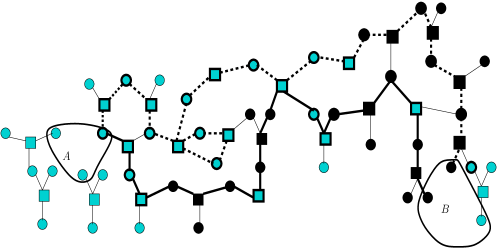
Figure 1: Each set $A$ and $B$ contains three variable nodes. The light squares denote the generator bits in the complement of $\mathcal{B}$ and the dark squares denote the generator bits in $\mathcal{B}$. The thick path is an example of a self-avoiding path between $A$ and $B$ which contributes to the upper bound. The dashed path is a non-self-avoiding path and does not contribute to the bound.

We use the following (see Appendix A for the proof)

Lemma 1.

Consider any LDGM code with bounded left and right degree. Consider two sets of information-bit nodes $A$, $B$ with bounded support. We have

$$\big{|}\langle\prod_{a\in A}u_{a}\prod_{b\in B}u_{b}\rangle-\langle\prod_{a\in A}u_{a}\rangle\langle\prod_{b\in B}u_{b}\rangle\big{|}\leq 2\sum_{w\in W_{AB}}\prod_{i\in w}\rho_{i}$$ (16)

where $\rho_{i}=1$, if $i\in\mathcal{B}$ and $\rho_{i}=e^{4|l_{i}|}-1$, if $i\notin\mathcal{B}$.

The crucial feature of this lemma is that the $\rho_{i}$ are independent random variables because the walks are self-avoiding. Consequently, averaging over the noise realization in (16)

$$\mathbb{E}_{l^{n}}\big{|}\langle\prod_{a\in A}u_{a}\prod_{b\in B}u_{b}\rangle-\langle\prod_{a\in A}u_{a}\rangle\langle\prod_{b\in B}u_{b}\rangle\big{|} \leq 2\sum_{w\in W_{AB}}\prod_{i\in w}\mathbb{E}[\rho_{i}]$$ (17)

Now,

$$\mathbb{E}[\rho_{i}] \leq\mathbb{E}[\rho_{i}\mid i\notin\mathcal{B}]\mathbb{P}(i\notin\mathcal{B})+\mathbb{E}[\rho_{i}\mid i\in\mathcal{B}]\mathbb{P}(i\in\mathcal{B})$$ (18)

$$\leq(e^{4H}-1)+\mathbb{P}\big{(}|l|>H\big{)}=\delta(\epsilon,H)$$ (19)

For our class of channels we can choose $H=H(\epsilon)$ such that $K\delta(\epsilon,H(\epsilon))<1$. We get

$$\mathbb{E}_{l^{n}}\big{|}\langle\prod_{a\in A}u_{a}\prod_{b\in B}u_{b}\rangle-\langle\prod_{a\in_{A}}u_{a}\rangle\langle\prod_{b\in_{B}}u_{b}\rangle\big{|} \leq 2\sum_{w\in W_{AB}}\delta(\epsilon)^{|w|}$$ (20)

$$\leq 2|A||B|\sum_{d\geq{\rm dist}(A,B)}(K\delta(\epsilon,H(\epsilon)))^{d}$$ (21)

$$\leq\frac{2|A||B|}{1-K\delta(\epsilon,H(\epsilon))}(K\delta(\epsilon))^{\text{dist}(A,B)}$$ (22)

The second inequality is obtained by noticing that the number of selfavoiding random walks of length $|w|$ is certainly bounded by $K^{|w|}$. The factor $|A||B|$ accounts for the maximum possible number of initial and final vertices. The correlation decay of the theorem is in fact a special case of this last bound for the choice $A=\partial i$ and $B=\partial j$. ∎

We now look at GEXIT functions of the MAP and BP decoders. For LDGM codes the functional giving the MAP-GEXIT function in (9) is

$$\mathcal{G}(\langle x_{i}\rangle_{0})=\frac{\Lambda^{\prime}(1)}{P^{\prime}(1)}\int dl_{i}\frac{dc(l_{i})}{d\epsilon}\mathbb{E}_{l^{n\setminus i}}\ln\biggl{\{}\frac{1+\langle x_{i}\rangle_{0}\tanh l_{i}}{1+\tanh l_{i}}\biggr{\}}$$ (23)

Derivations of this formula can be found in [1], [13].

The BP-GEXIT curve is given by the same functionals with $\langle x_{i}\rangle_{0}$ replaced by $\langle x_{i}\rangle_{0,d}^{BP}$. Consider $N_{d}(i)$ the neigborhood of node $i$, radius $d$ an even integer (all the vertices at graph-distance less or equal to $d$ from $i$). As is well known for an ensemble LDGM($\Lambda,P$) with bounded degrees, given $d$, if $n$ is large enough, the probability that $N_{d}(i)$ is a tree is $1-O(\frac{\gamma^{d}}{n})$ (where $\gamma$ depends only on $l_{\max},k_{\max}$). Thus when $d$ is fixed and $n\to+\infty$ the computational tree $T_{d}(i)$ and the neighborhood $N_{d}(i)$ match with high probability. This implies that

$$\lim_{d\to+\infty}\lim_{n\to+\infty}g_{n,d}^{BP}(\epsilon)=\mathbb{E}_{\mathcal{C}}[\mathcal{G}(\langle x_{i}\rangle_{0,N_{d}(i)})|N_{d}(i)\,\text{is a tree}]$$ (24)

where $\langle x_{i}\rangle_{0,N_{d}(i)}$ is the Gibbs bracket associated to the subgraph $N_{d}(i)$. The right hand side can exactly computed by performing the statistical mechanical sums on a tree and yields the DE formulas

$$\lim_{d\to+\infty}\lim_{n\to+\infty}g_{n,d}^{BP}(\epsilon)=\lim_{d\to\infty}\frac{\Lambda^{\prime}(1)}{P^{\prime}(1)}\int dl\frac{dc(l)}{d\epsilon}\mathbb{E}_{\Delta^{(d)}}\ln\bigg{\{}\frac{1+\tanh\Delta^{(d)}\tanh l}{1+\tanh l}\bigg{\}}$$ (25)

where both limits exist and

$$\tanh\Delta^{(d)}=\prod_{i=1}^{k}\tanh v_{i}^{(d)}$$ (26)

The $v_{i}^{(d)}$ are i.i.d random variables with distribution obtained from the iterative system of DE equations

$$\eta^{(d)}(v) =\sum_{l}\frac{l\Lambda_{l}}{\Lambda^{\prime}(1)}\int\prod_{i=1}^{l-1}du_{i}\,\widehat{\eta}^{(d)}(u_{i})\delta(v-\sum_{i=1}^{l-1}u_{i})$$ (27)

$$\widehat{\eta}^{(d)}(u) =\sum_{k}\frac{kP_{k}}{P^{\prime}(1)}\int dlc(l)\prod_{a=1}^{k-1}dv_{a}\,\eta^{(d-1)}(v_{a})\delta(u-\tanh^{-1}(\tanh l\prod_{i=1}^{k-1}\tanh v_{a})$$ (28)

with the initial condition $\eta^{(0)}(v)=\delta(v)$. It is well known that these equations are an iterative version of the replica fixed point equation [23].

Proof of corollary 1, LDGM.

Expanding the logarithm in (23) and using Nishimori identities as in [13] we obtain the expansion

$$\frac{\Lambda^{\prime}(1)}{P^{\prime}(1)}\sum_{p=1}^{+\infty} \frac{T_{2p}(\epsilon)}{2p(2p-1)}\bigl{(}\mathbb{E}_{\mathcal{C},l^{n\setminus i}}[\langle x_{i}\rangle^{2p}_{0}]-1\bigr{)}$$ (29)

where we recall that

$$T_{2p}(\epsilon)=\frac{d}{d\epsilon}\int_{-\infty}^{+\infty}dl\,c(l)(\tanh l)^{2p}$$ (30)

Note that in order to get the above expansion, it is important to use (23) as expressed here in terms of the extrinsic estimate. Obviously, the series is absolutely convergent, uniformly with respect to $n$, for the class of channels $\mathcal{K}$. Thus by dominated convergence, the proof will be complete if we show that

$$\lim_{n\to+\infty}\mathbb{E}_{\mathcal{C},l^{n\setminus i}}[\langle x_{i}\rangle^{2p}_{0}]=\lim_{d\to+\infty}\mathbb{E}_{\Delta^{(d)}}[(\tanh\Delta^{(d)})^{2p}]$$ (31)

Indeed one can then compute the $n\to+\infty$ limit term by term in (29) and then resum the resulting series (which is again absolutely convergent, uniformly with respect to $d$) to obtain (25).

Let us show (31). As pointed out before for $d$ fixed and $n\to+\infty$, $N_{d}(i)$ is a tree with high probability. Thus,

$$\lim_{n\to\infty}\mathbb{E}_{\mathcal{C},l^{n\setminus i}}[\langle x_{i}\rangle^{2p}_{0}]=\lim_{n\to\infty}\mathbb{E}_{\mathcal{C},l^{n\setminus i}}[\langle x_{i}\rangle^{2p}_{0}|N_{d}(i)\,\text{is a tree}]$$ (32)

Notice that all paths connecting the bit $i$ with those outside $N_{d}(i)$ have a length at least equal to $d$, so because of Theorem 1 in the high noise regime $x_{i}$ is very weakly correlated to the complement of $N_{d}(i)$. Therefore we may expect that

$$\lim_{d\to+\infty}\lim_{n\to+\infty}\mathbb{E}_{\mathcal{C},l^{n\setminus i}}[|\langle x_{i}\rangle_{0}^{2p}-\langle x_{i}\rangle_{0,N_{d}(i)}^{2p}|\mid N_{d}(i)\,\text{tree}]=0$$ (33)

Assuming for a moment that this is true we get from (32),

$$\lim_{n\to\infty}\mathbb{E}_{\mathcal{C},l^{n\setminus i}}[\langle x_{i}\rangle^{2p}_{0}]=\lim_{d\to\infty}\lim_{n\to\infty}\mathbb{E}_{\mathcal{C},l^{n\setminus i}}[\langle x_{i}\rangle^{2p}_{0,N_{d}(i)}|N_{d}(i)\,\text{is a tree}]$$ (34)

and, when $N_{d}(i)$ is a tree, the Gibbs average $\langle x_{i}\rangle^{2p}_{0,N_{d}(i)}$ is explicitly computable and the right hand side of (34) reduces to

$$\lim_{d\to+\infty}\mathbb{E}_{\Delta^{(d)}}[(\tanh\Delta^{(d)})^{2p}]$$ (35)

This proves (31).

Our task is now to prove (33). Let $\mathring{N}_{d}(i)$ be the set of checks that are at distance $d$ from $i$. We order the checks $\in\mathring{N}_{d}(i)$ in a given (arbitrary) way, and call $\langle-\rangle_{0;\leq k}$ the Gibbs average with $l_{k}=0$ for the $k$ first checks of $\mathring{N}_{d}(i)$ (and $l_{i}=0$ for the root node). For the first one (call it $1$) we use $e^{l_{1}x_{1}}=\cosh l_{1}+x_{1}\sinh l_{1}$ to find

$$\langle x_{i}\rangle_{0}=\langle x_{i}\rangle_{0;\leq 1}+\frac{\tanh l_{1}\big{(}\langle x_{i}x_{1}\rangle_{0;\leq 1}-\langle x_{i}\rangle_{0;\leq 1}\langle x_{1}\rangle_{0;\leq 1}\big{)}}{1+\langle x_{1}\rangle_{0;\leq 1}\tanh l_{1}}$$ (36)

Therefore

$$|\langle x_{i}\rangle_{0}^{2p}-\langle x_{i}\rangle_{0;\leq 1}^{2p}| \leq 2p|\langle x_{i}\rangle_{0}-\langle x_{i}\rangle_{0;\leq 1}|$$ (37)

$$\leq 2p\,t_{1}|\langle x_{i}x_{1}\rangle_{0;\leq 1}-\langle x_{i}\rangle_{0;\leq 1}\langle x_{1}\rangle_{0;\leq 1}|$$ (38)

where

$$t_{k}=\frac{|\tanh l_{k}|}{1-|\tanh l_{k}|}$$ (39)

We can now take the second check of $\mathring{N}_{d}(i)$ (call it $2$) and show

$$|\langle x_{i}\rangle_{0;\leq 1}^{2p}-\langle x_{i}\rangle_{0;\leq 2}^{2p}|\leq 2p\,t_{2}|\langle x_{i}x_{2}\rangle_{0;\leq 2}-\langle x_{i}\rangle_{0;\leq 2}\langle x_{2}\rangle_{0;\leq 2}|$$ (40)

We can repeat this argument for all nodes of $\partial N_{d}(i)$ and use the triangle inequality to obtain

$$|\langle x_{i}\rangle_{0}^{2p}-\langle x_{i}\rangle_{0,N_{d}(i)}^{2p}|\leq 2p\sum_{k\in\mathring{N}_{d}(i)}t_{k}|\langle x_{i}x_{k}\rangle_{0;\leq k}-\langle x_{i}\rangle_{0;\leq k}\langle x_{k}\rangle_{0;\leq k}|$$ (41)

Indeed the Gibbs average with all $l_{k}=0$ for all $k\in\mathring{N}_{d}(i)$ is equal to $\langle x_{i}\rangle_{0,N_{d}(i)}$. Now using the bound (22) in the proof of theorem 1 for $K\delta(\epsilon)<1$, the last inequality implies

$$\mathbb{E}_{\mathcal{C},l^{n\setminus i}}[|\langle x_{i}\rangle_{0}^{2p}-\langle x_{i}\rangle_{0,N_{d}(i)}^{2p}|\mid N_{d}(i)\,\text{tree}]\leq\frac{4pK^{2}\mathbb{E}[t]}{1-K\delta(\epsilon)}K^{d}(K\delta(\epsilon))^{d}$$ (42)

Note that for channels $\mathcal{K}$, for non-zero noise,

$$\mathbb{E}[t]=\mathbb{E}\biggl{[}\frac{|\tanh l|}{1-|\tanh l|}\biggr{]}\leq\mathbb{E}[e^{2|l|}]<\infty$$ (43)

The right hand side of (42) does not depend on $n$, so it is immediate that $\lim_{d\to+\infty}\lim_{n\to+\infty}$ vanishes as long as the noise is high enough such that $K^{2}\delta(\epsilon)<1$. This proves (33) and the corollary. ∎

To conclude, let us remark that, for the BIAWGNC the GEXIT formulas simplify considerably and there is a clear relationship to the magnetization,

$$\mathcal{G}(\langle x_{i}\rangle) =\frac{1}{\epsilon^{3}}\frac{\Lambda^{\prime}(1)}{P^{\prime}(1)}\big{(}1-\mathbb{E}_{l^{n}}[\langle x_{i}\rangle]\big{)}$$ (44)

$$=\frac{1}{\epsilon^{3}}\frac{\Lambda^{\prime}(1)}{P^{\prime}(1)}(1-\mathbb{E}_{l^{n}}[\tanh(l+\tanh^{-1}\langle x_{i}\rangle_{0})])$$ (45)

and

$$\lim_{d\to+\infty}\lim_{n\to+\infty}g_{n,d}^{BP}(\epsilon)=\frac{1}{\epsilon^{3}}\frac{\Lambda^{\prime}(1)}{P^{\prime}(1)}(1-\mathbb{E}_{l,\Delta^{(d)}}[\tanh(l+\Delta^{(d)})])$$ (46)

The proof of corrolary 1 for BIAWGNC can thus proceed without expansions and is slightly simpler. The main ideas can be found in [17] and we do not repeat them here. Note also that for the BEC there are similar simplifications that occur: this allows us to make a proof which avoids the second condition in the class of channels $\mathcal{K}$.

4 LDPC Codes: Low Noise

In this section we prove theorem 1 and corollary 1 for LDPC codes in a low noise regime. As explained in section 2 we first transform the problem to a dual one. The duality transformation reviewed here essentially is an application of Poisson’s summation formula over commutative groups, and has been thoroughly discussed in the context of codes on graphs in [24]. Here we need to know how the correlations transform under the duality, a point that does not seem to appear in the related literature.

4.1 Duality formulas for the correlations

Let $C$ be a binary parity check code and $C^{\perp}$ its dual. We apply the Poisson summation formula

$$\sum_{x^{n}\in C}f(x^{n})=\frac{1}{|C|}\sum_{\tau^{n}\in C^{\perp}}\widehat{f}(\tau^{n})$$ (47)

where the Fourier (or Hadamard) transform is,

$$\widehat{f}(\tau^{n})=\sum_{x^{n}\in\{-1,+1\}^{n}}f(x^{n})e^{i\frac{\pi}{4}\sum_{j=1}^{n}(1-\tau_{j})(1-x_{j})}$$ (48)

to the partition function $Z$ of an LDPC code $C$. The dual code $C^{\perp}$ is an LDGM with codewords given by $\tau^{n}$ where

$$\tau_{i}=\prod_{a\in\partial i}u_{a}$$ (49)

and $u_{a}$ are the $m$ information bits. A straigthforward application of the Poisson formula then yields the extended form of the MacWilliams identity,

$$Z=\frac{1}{|C^{\perp}|}e^{\sum_{j=1}^{n}l_{j}}Z_{\perp}$$ (50)

where

$$Z_{\perp}=\sum_{u^{m}\in\{-1,+1\}^{m}}\prod_{i=1}^{n}(1+e^{-2l_{i}}\prod_{a\in\partial i}u_{a})$$ (51)

This expression formaly looks like the partition function of an LDGM code with “channel half-loglikelihoods” $g_{i}$ such that $\tanh g_{i}=e^{-2l_{i}}$. This is truly the case only for the BEC($\epsilon$) where $l_{i}=0,+\infty$ and hence $g_{i}=+\infty,0$ which still correspond to a BEC($1-\epsilon$). The logarithm of partition functions is related to the input-output entropy and one recovers (taking the $\epsilon$ derivative) the well known duality relation between EXIT functions of a code and its dual on the BEC [25]. For other channels however this is at best a formal (but still useful) analogy since the weights are negative for $l_{i}<0$ (and $g_{i}$ takes complex values). We introduce a bracket $\langle-\rangle_{\perp}$ which is not a true probabilistic expectation (but it is still linear)

$$\langle f\rangle_{\perp}=\frac{1}{Z_{\perp}}\sum_{u^{m}\in\{-1,+1\}^{m}}f(u^{m})\prod_{i=1}^{n}(1+e^{-2l_{i}}\prod_{a\in i}u_{a})$$ (52)

The denominator may vanish, but it can be shown that when this happens the numerator also does so in a way that ensures the finiteness of the ratio (this becomes clear in subsequent calculations). Taking logarithm of (50) and then the derivative with respect to $l_{i}$ we find

$$\langle x_{i}\rangle =\frac{1}{\tanh 2l_{i}}-\frac{\langle\tau_{i}\rangle_{\perp}}{\sinh 2l_{i}}$$ (53)

and differentiating once more with respect to $l_{j}$, $j\neq i$

$$\langle x_{i}x_{j}\rangle-\langle x_{i}\rangle\langle x_{j}\rangle=\frac{\langle\tau_{i}\tau_{j}\rangle_{\perp}-\langle\tau_{i}\rangle_{\perp}\langle\tau_{j}\rangle_{\perp}}{\sinh 2l_{i}\sinh 2l_{j}}$$ (54)

We stress that in (53), (54), $\tau_{i}$ and $\tau_{j}$ are given by products of information bits (49). The left hand side of (53) is obviously bounded. It is less obvious to see this directly on the right hand side and here we just note that the pole at $l_{i}=0$ is harmless since, for $l_{i}=0$, the bracket has all its “weight“ on configurations with $\tau_{i}=1$. Similar remarks apply to (54). In any case, we will beat the poles by using the following trick. For any $0<s<1$ and $|a|\leq 1$ we have $|a|\leq|a|^{s}$, thus

$$\mathbb{E}_{l^{n}}[|\langle x_{i}x_{j}\rangle-\langle x_{i}\rangle\langle x_{j}\rangle|]\leq 2^{1-s}\mathbb{E}_{l^{n}}[|\langle x_{i}x_{j}\rangle-\langle x_{i}\rangle\langle x_{j}\rangle|^{s}]$$

and using (54) and Cauchy-Schwarz

$$\mathbb{E}_{l^{n}}[|\langle x_{i}x_{j}\rangle-\langle x_{i}\rangle\langle x_{j}\rangle|]\leq 2^{1-s}\mathbb{E}[(\sinh 2l)^{-2s}]\mathbb{E}_{l^{n}}[|\langle\tau_{i}\tau_{j}\rangle_{\perp}-\langle\tau_{i}\rangle_{\perp}\langle\tau_{j}\rangle_{\perp}|^{2s}]^{1/2}$$ (55)

The prefactor is always finite for $0\leq s<\frac{1}{2}$ for our class of channels $\mathcal{K}$. For example for the BIAWGNC we have

$$\mathbb{E}[(\sinh 2l)^{-2s}]\leq\frac{c}{|1-2s|}e^{-c^{\prime}\frac{s(1-2s)}{\epsilon^{2}}}$$ (56)

for purely numerical constants $c,c^{\prime}>0$ and for the BSC we have

$$\mathbb{E}[(\sinh 2l)^{-2s}]\leq\biggl{(}\frac{2\epsilon(1-\epsilon)}{1-2\epsilon}\biggr{)}^{2s}$$ (57)

4.2 Decay of correlations for low noise

We will prove the decay of correlations by applying a high temperature cluster expansion technique to $\mathbb{E}_{l^{n}}[|\langle\tau_{i}\tau_{j}\rangle_{\perp}-\langle\tau_{i}\rangle_{\perp}\langle\tau_{j}\rangle_{\perp}|^{2s}]$. As explained in section 2 we need a technique that does not use the positivity of the Gibbs weights. In appendix B we give a streamlined derivation of an adaptation of Berretti’s expansion.

$$\langle\tau_{i}\tau_{j}\rangle_{\perp}-\langle\tau_{i}\rangle_{\perp}\langle\tau_{j}\rangle_{\perp}=\frac{1}{2}\sum_{\hat{X}}K_{i,j}(\hat{X})\Bigl{(}\frac{Z_{\perp}(\hat{X}^{c})}{Z_{\perp}}\Bigr{)}^{2}$$ (58)

where

$$K_{i,j}(\hat{X})\equiv\sum_{\begin{subarray}{c}u_{a}^{(1)},u^{(2)}_{a}\\ a\in\hat{X}\end{subarray}}\sum_{\begin{subarray}{c}\Gamma~{}\text{compatible}\\ \text{with}\hat{X}\end{subarray}}(\tau_{i}^{(1)}-\tau_{i}^{(2)})(\tau_{j}^{(1)}-\tau_{j}^{(2)})\prod_{k\in\Gamma}E_{k}$$ (59)

and

$$E_{k}=\tau_{k}^{(1)}e^{-2l_{k}}+\tau_{k}^{(2)}e^{-2l_{k}}+\tau_{k}^{(1)}\tau_{k}^{(2)}e^{-4l_{k}}$$ (60)

Here $u_{a}^{(1)}$ and $u_{a}^{(2)}$ are two independent copies of the information bits (these are also known as real replicas) and $\tau_{k}^{(\alpha)}=\prod_{a\in k}u_{a}^{(\alpha)}$. To explain what are $\hat{X}$ and $\Gamma$ we will refer to $a$-nodes (check nodes in the Tanner graph representing the LDPC code) and $i$-nodes (variable nodes in the Tanner graph representing the LDPC code). Given a subset $S$ of nodes of the graph let $\partial S$ be the subset of neighboring nodes. In (58) the sum over $\hat{X}$ is carried over clusters of $a$-nodes such that “$\hat{X}$ is connected via hyperedges”: this means that a) $\hat{X}=\partial X$ for some connected subset $X$ of $i$-nodes; b) $X$ is connected if any pair of $i$-nodes can be joined by a path all of whose variable nodes lie in $X$; c) $\hat{X}$ contains both $\partial i$ and $\partial j$. In the sum (59) $\Gamma$ is a set of $i$-nodes (all distinct). We say that “$\Gamma$ is compatible with $\hat{X}$” if: (i) $\partial\Gamma\cup\partial i\cup\partial j=\hat{X}$, (ii) $\partial\Gamma\cap\partial i\neq\phi$ and $\partial\Gamma\cap\partial j\neq\phi$, (iii) there is a walk connecting $\partial i$ and $\partial j$ such that all its variable nodes are in $\Gamma$. Finally,

$$Z_{\perp}(\hat{X}^{c})=\sum_{\begin{subarray}{c}u_{a}\\ a\in\hat{X}^{c}\end{subarray}}\prod_{\begin{subarray}{c}\text{all}\;i\;\text{s.t.}\\ \partial i\cap\hat{X}=\phi\end{subarray}}(1+e^{-2l_{i}}\prod_{a\in i}u_{a})$$ (61)

The figure Fig. 2 gives an example for all the sets appearing above.

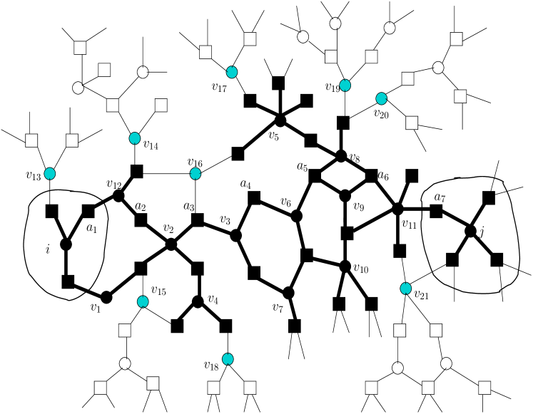
Figure 2: In this figure we explain the various sets appearing in the cluster expansion (58). The Tanner graph represents the LDPC code with variable nodes ($i$-nodes) denoted by circles and check nodes ($a$-nodes denoted by squares). In this example the set $\hat{X}$ is the set of dark check nodes. It is easy to verify that this choice of $\hat{X}$ satisfies all our conditions. Firstly, let $X=\{i,j,v_{1},v_{2},v_{3},v_{4},v_{5},v_{6},v_{7},v_{8},v_{9},v_{10},v_{11},v_{12}\}$ be a set of variable nodes (these are denoted by dark circles in the figure). It is easy to check that the set of neighbours of $X$ is given by the dark check nodes which is $\hat{X}$. Hence $\hat{X}=\partial X$. Secondly, any two variable nodes in $X$ are connected by a path all of whose variable nodes lie in $X$, and thirdly, $\hat{X}$ contains both $\partial i$ and $\partial j$. One choice for $\Gamma=\{v_{2},v_{3},v_{4},v_{5},v_{6},v_{7},v_{8},v_{10},v_{11},v_{12}\}$. It is easy to check that $\Gamma$ is compatible with $\hat{X}$. The walk $\{a_{1}v_{12}a_{2}v_{2}a_{3}v_{3}a_{4}v_{6}a_{5}v_{8}a_{6}v_{11}a_{7}\}$ connects $\partial i$ and $\partial j$ and all its variable nodes lie in $\Gamma$. Another choice for $\Gamma$ would be the set $\{v_{2},v_{3},v_{4},v_{5},v_{6},v_{7},v_{8},v_{9},v_{10},v_{11},v_{12}\}$. In the definition of $Z_{\perp}(\hat{X}^{c}),Z(\hat{X}^{c})$ the light variable nodes, $v_{13},v_{14},v_{15},v_{16},v_{17},v_{18},v_{19},v_{20},v_{21}$, are not present because they have a non-empty intersection with $\hat{X}$.

We are now ready to prove the theorem on decay of correlations.

Proof of theorem 1, LDPC.

Because of (55) it suffices to prove that
$\mathbb{E}_{l^{n}}[|\langle\tau_{i}\tau_{j}\rangle_{\perp}-\langle\tau_{i}\rangle_{\perp}\langle\tau_{j}\rangle_{\perp}|^{2s}]$ decays.

The first step is to prove

$$\biggl{|}\frac{Z_{\perp}(\hat{X}^{c})}{Z_{\perp}}\biggr{|}\leq 1$$ (62)

This ratio is not easily estimated directly because the weights in $Z_{{\mathcal{C}}^{\perp}}$ are not positive. However we can use the duality transformation (50) backwards to get a new ratio of partition functions with positive weights,

$$\frac{Z_{\perp}(\hat{X}^{c})}{Z_{\perp}}=\biggl{(}\exp{\sum_{\begin{subarray}{c}\text{all}\,i\,\text{s.t}\\ \partial i\cap\hat{X}\neq\phi\end{subarray}}l_{i}}\biggr{)}\frac{|C^{\perp}(\hat{X}^{c})|}{|C^{\perp}|}\frac{Z(\hat{X}^{c})}{Z}$$ (63)

with

$$Z(\hat{X}^{c})=\sum_{\begin{subarray}{c}x_{i}\\ \partial i\cap\hat{X}=\phi\end{subarray}}\prod_{\begin{subarray}{c}\text{all}\,i\,\text{s.t}\\ \partial i\cap\hat{X}=\phi\end{subarray}}e^{l_{i}x_{i}}\prod_{a\in\hat{X}^{c}}\frac{1}{2}(1+\prod_{\begin{subarray}{c}i\in a\,\text{and}\\ \partial i\cap\hat{X}=\phi\end{subarray}}x_{i})$$ (64)

This is the partition function corresponding to the subgraph induced by $a$-nodes of $\hat{X}^{c}$ and $i$-nodes such that $i\,\text{s.t}\,\partial i\cap\hat{X}=\phi$. Moreover $C^{\perp}(\hat{X}^{c})$ is the dual of the later code $C(\hat{X}^{c})$ defined on the subgraph. By standard properties of the rank of a matrix, the rank of the parity check matrix of $C(\hat{X}^{c})$, which is obtained by removing rows (checks) and columns (variables) from the parity check matrix of $C$, is smaller than the rank of the parity check matrix of $C$. This implies $|C^{\perp}(\hat{X}^{c})|\leq|C^{\perp}|$. Moreover

$$\biggl{(}\exp{\sum_{\begin{subarray}{c}\text{all}\,i\,\text{s.t}\\ \partial i\cap\hat{X}\neq\phi\end{subarray}}l_{i}}\biggr{)}Z(\hat{X}^{c})\leq Z$$ (65)

To see this one must recognize that the left hand side is the sum of terms of $Z$ corresponding to $\sigma^{n}$ such that $\sigma_{i}=+1$ for $\partial i\cap\hat{X}\neq\phi$ (and all terms are $\geq 0$). These remarks imply (62).

Using $|\sum_{i}a_{i}|^{2s}\leq\sum_{i}|a_{i}|^{2s}$ for $0<2s<1$ and (62) we find

$$\mathbb{E}_{l^{n}}[|\langle\tau_{i}\tau_{j}\rangle_{\perp}-\langle\tau_{i}\rangle_{\perp}\langle\tau_{j}\rangle_{\perp}|^{2s}]\leq\frac{1}{2^{2s}}\sum_{\hat{X}}\mathbb{E}_{l^{n}}\bigl{[}|K_{i,j}(\hat{X})|^{2s}\bigr{]}$$ (66)

Trivially bounding the spins in $\eqref{eq:Ea}$ we deduce

$$\mathbb{E}_{l^{n}}\bigl{[}|K_{i,j}(\hat{X})|^{2s}\bigr{]} \leq 4^{|\hat{X}|}\sum_{\begin{subarray}{c}\Gamma~{}\text{compatible}\\ \text{with}\hat{X}\end{subarray}}(2^{2s}\mathbb{E}[e^{-4sl}]+\mathbb{E}[e^{-8sl}])^{|\Gamma|}$$

$$\leq 4^{|\hat{X}|}\sum_{\begin{subarray}{c}\Gamma~{}\text{compatible}\\ \text{with}\hat{X}\end{subarray}}2^{(4s+1)|\Gamma|}\Delta(\epsilon)^{|\Gamma|}$$ (67)

where

$$\Delta(\epsilon)=2^{2s}\mathbb{E}[e^{-4sl}]+\mathbb{E}[e^{-8sl}]$$ (68)

Since $\Gamma$ is compatible with $\hat{X}$ we necessarily have $|\partial\Gamma|\geq|\hat{X}|-|\partial i|-|\partial j|$ and since $|\partial\Gamma|\leq|\Gamma|l_{\max}$, we get $|\Gamma|\geq(|\hat{X}|-2l_{\max})/l_{\max}$. Also, the maximum number of $a$-nodes which have an intersection with $\hat{X}$ is $|\hat{X}|k_{\max}$. Thus there are at most $2^{|\hat{X}|k_{\max}}$ possible choices for $\Gamma$. These remarks imply

$$\mathbb{E}_{l^{n}}\bigl{[}|K_{i,j}(\hat{X})|^{2s}\bigr{]}\leq 2^{(2+k_{\max})|\hat{X}|}\Delta(\epsilon)^{(|\hat{X}|-2l_{\max})/l_{\max}}$$ (69)

From (66) and (69) we get

$$\mathbb{E}_{l^{n}}[|\langle\tau_{i}\tau_{j}\rangle_{\perp}-\langle\tau_{i}\rangle_{\perp}\langle\tau_{j}\rangle_{\perp}|^{2s}]\leq\frac{1}{2^{2s}}\sum_{\hat{X}}2^{(2+k_{\max})|\hat{X}|}\Delta(\epsilon)^{(|\hat{X}|-2\texttt{l}_{\text{max}})/2\texttt{l}_{\text{max}}}$$ (70)

The clusters $\hat{X}$ connect $\partial i$ and $\partial j$ and thus have sizes $|\hat{X}|\geq\frac{1}{2}\text{dist}(i,j)$. Moreover the number of clusters of a given size grows at most like $K^{|\hat{X}|}$ where $K=l_{\max}k_{max}$. Since for the class $\mathcal{K}$ we have for $s$ small enough, $\mathbb{E}[e^{sl}]\to 0$ as $\epsilon\to 0$ we can always chose $\epsilon$ small enough to make $\Delta(\epsilon)$ small enough and conclude the proof. ∎

4.3 Density evolution equals MAP for low noise

In the case of LDPC codes the functional giving the MAP-GEXIT function in (9) is [14]

$$\mathcal{G}(\langle x_{i}\rangle_{0})==\int dl_{i}\frac{dc(l_{i})}{d\epsilon}\mathbb{E}_{l^{n\setminus i}}\ln\biggl{\{}\frac{1+\langle x_{i}\rangle_{0}\tanh l_{i}}{1+\tanh l_{i}}\biggr{\}}$$ (71)

Note that the only formal difference with the LDGM case is in the normalization factor; but of course now the Gibbs average pertains to the LDPC measure. The BP-GEXIT curve is given by the same functionals with $\langle x_{i}\rangle_{0}$ replaced by the average on the computational tree $\langle x_{i}\rangle_{0,d}^{BP}$. As in section 3 we introduce $N_{d}(i)$ the neigborhood of node $i$, radius $d$ an even integer. By the same arguments than in section 3 we have again

$$\lim_{d\to+\infty}\lim_{n\to+\infty}g_{n,d}^{BP}(\epsilon)=\mathbb{E}_{C}[\mathcal{G}(\langle x_{i}\rangle_{0,N_{d}(i)})|N_{d}(i)\,\text{is a tree}]$$ (72)

where $\langle x_{i}\rangle_{0,N_{d}(i)}$ is the Gibbs bracket associated to the graph $N_{d}(i)$. It is important to note that for $N_{d}(i)$ a tree the set of leaves $\mathring{N}_{d}(i)$ are variable nodes and have “natural boundary conditions” as given by the channel outputs. The statistical mechanical sums on a tree yield the DE formula

$$\lim_{d\to+\infty}\lim_{n\to+\infty}g_{n,d}^{BP}(\epsilon)=\lim_{d\to\infty}\int dl\frac{dc(l)}{d\epsilon}\mathbb{E}_{\Lambda^{(d)}}\ln\bigg{\{}\frac{1+\tanh\Lambda^{(d)}\tanh l}{1+\tanh l}\bigg{\}}$$ (73)

where both limits exist and

$$\Lambda^{(d)}=\sum_{a=1}^{k}w_{a}^{(d)}$$ (74)

The $w_{a}^{(d)}$ are i.i.d random variables with distribution obtained from the iterative system of DE equations

$$\zeta^{(d)}(w) =\sum_{l}\frac{l\Lambda_{l}}{\Lambda^{\prime}(1)}\int\prod_{j=1}^{l-1}d\lambda_{j}\,\zeta^{(d)}(\lambda_{j})\,\delta(w-\tanh^{-1}\bigl{(}\prod_{j=1}^{l-1}\tanh\lambda_{j}\bigr{)})$$

$$\widehat{\zeta}^{(d)}(\lambda) =\sum_{k}\frac{kP_{k}}{P^{\prime}(1)}\int dl\,c(l)\prod_{a=1}^{k-1}dw_{a}\,\zeta^{(d-1)}(w_{a})\,\delta(\lambda-l-\sum_{a=1}^{k-1}w_{a}^{(d)})$$

with the initial condition $\eta^{(0)}(\lambda)=c(\lambda)$. As before, these equations are an iterative version of the replica fixed point equation [23].

Proof of corollary 1, LDPC.

The first few steps are the same as in the proof for LDGM. First, we expand the logarithm in (71) and use Nishimori identities to obtain a series expansion like (29) (the prefactor $\frac{\Lambda^{\prime}(1)}{P^{\prime}(1)}$ is now absent). Second, we notice that since the resulting series expansion is uniformly absolutely convergent it is enough to show that

$$\lim_{n\to+\infty}\mathbb{E}_{\mathcal{C},l^{n\setminus i}}[\langle x_{i}\rangle^{2p}_{0}]=\lim_{d\to+\infty}\mathbb{E}_{d}[(\tanh\Lambda^{(d)})^{2p}]$$ (75)

Thirdly, as before, one argues that this follows from

$$\lim_{d\to+\infty}\lim_{n\to+\infty}\mathbb{E}_{C,l^{n\setminus i}}[|\langle x_{i}\rangle_{0}^{2p}-\langle x_{i}\rangle_{0,N_{d}(i)}^{2p}|\mid N_{d}(i)\,\text{tree}]=0$$ (76)

and because of $|b^{2p}-a^{2p}|\leq 2p|b-a|$ it is enough to show this for $2p$ replaced by $1$. Unfortunately one cannot proceed as simply as in the LDGM case: (76) is a consequence of the next two auxiliary lemmas stated below. ∎

Let $\langle-\rangle_{0;N_{d}(i)}^{\infty}$ be the bracket defined on the subgraph $N_{d}(i)$ with $l_{k}=+\infty$ for $k\in\partial N_{d}(i)$. This in fact is formaly equivalent to fixing $x_{k}=+1$ boundary conditions on the leaves of the tree $k\in\mathring{N}_{d}(i)$. The first lemma says that the bit estimate can be computed locally.

Lemma 2.

Under the same conditions than in corollary 1,

$$\lim_{d\to+\infty}\lim_{n\to+\infty}\mathbb{E}_{C,l^{n\setminus i}}[|\langle x_{i}\rangle_{0}-\langle x_{i}\rangle_{0,N_{d}(i)}^{\infty}|\mid N_{d}(i)\,\text{tree}]=0$$ (77)

The second lemma says that at low enough noise free and $+1$ boundary conditions are equivalent

Lemma 3.

Under the same conditions than in corollary 1,

$$\lim_{d\to+\infty}\lim_{n\to+\infty}\mathbb{E}_{C,l^{n\setminus i}}[\langle x_{i}\rangle_{0,N_{d}(i)}^{\infty}-\langle x_{i}\rangle_{0,N_{d}(i)}|\mid N_{d}(i)\,\text{tree}]=0$$ (78)

We prove the first lemma. It will then be clear that the proof of the second one is essentialy the same except that the original full graph is replaced by $N_{d}(i)$, and thus it will be spared.

Proof of lemma 2.

In (77) (and (78)) the root node $i$ has $l_{i}=0$ which turns out to be technically cumbersome because we really work in a low noise regime. For this reason we use

$$\langle x_{i}\rangle=\frac{\langle x_{i}\rangle_{0}+\tanh l_{i}}{1+\langle x_{i}\rangle_{0}\tanh l_{i}},\qquad\langle x_{i}\rangle_{N_{d}(i)}^{\infty}=\frac{\langle x_{i}\rangle_{0,N_{d}(i)}^{\infty}+\tanh l_{i}}{1+\langle x_{i}\rangle_{0,N_{d}(i)}^{\infty}\tanh l_{i}}$$ (79)

to deduce

$$\langle x_{i}\rangle_{0}-\langle x_{i}\rangle_{0,N_{d}(i)}^{\infty}=\frac{(1-(\tanh l_{i})^{2})(\langle x_{i}\rangle-\langle x_{i}\rangle_{N_{d}(i)}^{\infty})}{(1-\langle x_{i}\rangle\tanh l_{i})(1-\langle x_{i}\rangle_{N_{d}(i)}^{\infty}\tanh l_{i})}$$ (80)

This implies

$$|\langle x_{i}\rangle_{0}-\langle x_{i}\rangle_{0;N_{d}(i)}^{\infty}|\leq\frac{1+|\tanh l_{i}|}{1-|\tanh l_{i}|}\,|\langle x_{i}\rangle-\langle x_{i}\rangle_{N_{d}(i)}^{\infty}|$$ (81)

and averaging over the noise and using Cauchy-Schwarz,

$$\mathbb{E}_{l^{n}\setminus i}[|\langle x_{i}\rangle_{0}-\langle x_{i}\rangle_{0;N_{d}(i)}^{\infty}|] \leq 2\mathbb{E}[e^{4|l|}]^{1/2}\mathbb{E}_{l^{n}}[|\langle x_{i}\rangle-\langle x_{i}\rangle_{N_{d}(i)}^{\infty}|^{2}]^{1/2}$$ (82)

$$\leq 2\sqrt{2}\,\mathbb{E}[e^{8|l|}]^{1/2}\,\mathbb{E}_{l^{n}}[|\langle x_{i}\rangle-\langle x_{i}\rangle_{N_{d}(i)}^{\infty}|]^{1/2}$$ (83)

Let us now prove

$$\lim_{d\to+\infty}\lim_{n\to+\infty}\mathbb{E}_{C,l^{n}}[|\langle x_{i}\rangle-\langle x_{i}\rangle_{N_{d}(i)}^{\infty}|\mid N_{d}(i)\,\text{tree}]=0$$ (84)

We order the variable nodes at the boundary $\mathring{N}_{d}(i)$ and consider the corresponding vector of loglikelihoods with components $\in\mathring{N}_{d}(i)$. If the first $k-1$ components of this vector are $l_{1},...,l_{k-1}=+\infty$, the $k$-th component is $l_{k}^{\prime}$, and the other ones are i.i.d distributed as $c(l)$ (in other words they are “natural“) we write $\langle-\rangle_{\leq k-1}^{\infty}$. From the fundamental theorem of calculus, it is not difficult to see that

$$\langle x_{i}\rangle- \langle x_{i}\rangle_{N_{d}(i)}^{\infty}=-\sum_{k\in\mathring{N}_{d}(i)}\int_{l_{k}}^{+\infty}dl_{k}^{\prime}\,\frac{d}{dl_{k}^{\prime}}\langle x_{i}\rangle_{\leq k-1}^{\infty}$$ (85)

$$=-\sum_{k\in\mathring{N}_{d}(i)}\int_{l_{k}}^{+\infty}dl_{k}^{\prime}\,(\langle x_{i}x_{k}\rangle_{\leq k-1}^{\infty}-\langle x_{i}\rangle_{\leq k-1}^{\infty}\langle x_{k}\rangle_{\leq k-1}^{\infty})$$ (86)

Using $|a|\leq|a|^{s}$ for any $0<s<1$ and $|a|\leq 1$ we get

$$|\langle x_{i}\rangle- \langle x_{i}\rangle_{N_{d}(i)}^{\infty}|$$ (87)

$$\leq 2^{1-s}\sum_{k\in\mathring{N}_{d}(i)}\int_{l_{k}}^{+\infty}dl_{k}^{\prime}\,|\langle x_{i}x_{k}\rangle_{\leq k-1}^{\infty}-\langle x_{i}\rangle_{\leq k-1}^{\infty}\langle x_{k}\rangle_{\leq k-1}^{\infty}|^{s}$$ (88)

Let $\langle-\rangle_{\leq k-1}^{\infty,\perp}$ be the dual bracket (with the first $k$ components of $\mathring{N}_{d}(i)$ $l_{1}=...=l_{k-1}=+\infty$ and the $k$-th component equal to $l_{k}^{\prime}$). Because of (54) we have

$$|\langle x_{i}\rangle- \langle x_{i}\rangle_{N_{d}(i)}^{\infty}|$$ (89)

$$\leq 2^{1-s}\sum_{k\in N_{d}(i)}\int_{l_{k}}^{+\infty}dl_{k}^{\prime}\,\frac{|\langle\tau_{i}\tau_{k}\rangle_{\leq k-1}^{\infty,\perp}-\langle\tau_{i}\rangle_{\leq k-1}^{\infty,\perp}\langle\tau_{k}\rangle_{\leq k-1}^{\infty,\perp}|^{s}}{(\sinh 2l_{i}\sinh 2l_{k}^{\prime})^{2s}}$$ (90)

Note that the denominator in the integral is important to make the integral convergent for $l_{k}^{\prime}\to\infty$. Moreover at $l_{i}$ and $l_{k}^{\prime}=0$ is harmless as long as for $2s<1$. The next step is to use the cluster expansion in order to estimate

$$\mathbb{E}_{l^{n}}\biggl{[}\int_{l_{k}}^{+\infty}dl_{k}^{\prime}\,\frac{|\langle\tau_{i}\tau_{k}\rangle_{\leq k-1}^{\infty,\perp}-\langle\tau_{i}\rangle_{\leq k-1}^{\infty,\perp}\langle\tau_{k}\rangle_{\leq k-1}^{\infty,\perp}|^{s}}{(\sinh 2l_{i}\sinh 2l_{k}^{\prime})^{2s}}\biggr{]}$$ (91)

By following similar steps than in the proof of theorem 1 one obtains an upper bound similar to (69) except that the likelihoods of the end points are weighted differently and therefore there are two factors of $\Delta(\epsilon)$ (see (68)) replaced by

$$\mathbb{E}\biggl{[}\frac{2^{2s}e^{-4sl}+e^{-8sl}}{(\sinh 2l)^{-2s}}\biggr{]}<\infty\qquad{\rm and}\qquad\mathbb{E}\biggl{[}\int_{l}^{+\infty}dl^{\prime}\,\frac{2^{2s}e^{-4sl^{\prime}}+e^{-8sl^{\prime}}}{(\sinh 2l^{\prime})^{-2s}}\biggr{]}<\infty$$ (92)

Finally we can average over the code ensemble conditional on the event that $N_{d}(i)$ is a tree. Since the clusters $\hat{X}$ that connect $\partial i$ and $\partial k$, $k\in N_{d}(i)$ have size $|\hat{X}|k_{\max}$ we obtain the result as long as $\Delta(\epsilon)$ is small enough, for $\epsilon$ small enough. ∎

5 Large block length versus large number of iterations

In the LDGM case we prove the exchange of limits $d,n\to+\infty$ for the BSC channel. As will become clear one needs the decay of correlations (or covariance) of the Gibbs measure on the computational tree for $d\gg n$. Hence the likelihoods are not independent r.v: the proof of theorem 1 still goes through in the case of the BSC. The only difference is that in lemma 1 we can take $H>\frac{1}{2}\ln\frac{1-\epsilon}{\epsilon}$ such that $\mathcal{B}=\emptyset$ and $\rho_{\pi(j)}=e^{4|l_{\pi(j)}|}-1=\frac{4|1-2\epsilon|}{(1-|1-2\epsilon|)^{2}}$ for all $j\in T_{d}(i)$.

Lemma 4 (Decay of correlations for the BP decoder, LDGM on BSC).

Consider communication with a fixed general LDGM code with blocklength size $n$ and bounded degrees $l_{\max}$, $k_{\max}$, over the BSC($\epsilon$). We can find $c>0$, a small enough numerical constant such that for $l_{\max}k_{\max}|1-2\epsilon|<c$ we have, for any given realization of the channel outputs,

$$|\langle x_{i}x_{j}\rangle_{d}^{BP}-\langle x_{i}\rangle_{d}^{BP}\langle x_{j}\rangle_{d}^{BP}|\leq c_{1}e^{-c_{2}(\epsilon){\rm dist}(i,j)}$$ (93)

where $i$ is the root of the computational tree, $j$ and arbitrary node, $c_{1}>0$ a numerical constant and $c_{2}(\epsilon)>0$ depending only on $\epsilon$, $l_{\max}$, $k_{\max}$. Moreover $c_{2}(\epsilon)$ increases like $\ln|1-2\epsilon|$ as $\epsilon\to\frac{1}{2}$.

Basically, this result is contained in [22] where it is obtained by Dobrushin’s criterion. Note that it is valid for fixed noise realizations and not only on average. The unbounded case would require to take averages but then, on the computational tree one has to control moments $\mathbb{E}[\rho_{\pi}(i)^{m}]$ and this requires more work. The following proof is a simple application of this lemma.

Proof of theorem 2, LDGM, BSC.

We take for the number of iterations of the BP decoder $d\gg n$. On the computational tree $T_{d}(i)$ we consider the subtree of root $i$ and depth $d^{\prime}\ll n$. This subtree is a smaller computational tree $T_{d^{\prime}}(i)\subset T_{d}(i)$ and $d^{\prime}\ll n\ll d$. Let $\mathring{T}_{d^{\prime}}(i)$ the leaves $k$ with ${\rm dist}(i,k)=d^{\prime}$ and order them in an arbitrary way. Consider the Gibbs measure $\langle-\rangle_{d;\leq k}^{BP}$ where for the first $k$ checks of $\mathring{T}_{d^{\prime}}(i)$ we set $l_{\pi(k)}=0$ in (10). Proceeding as in section 3 we get

$$|\langle x_{i}\rangle_{d}^{BP}-\langle x_{i}\rangle_{d^{\prime}}^{BP}|\leq\sum_{k\in\mathring{T}_{d^{\prime}}(i)}t_{\pi(k)}|\langle x_{i}x_{k}\rangle_{d;\leq k}^{BP}-\langle x_{i}\rangle_{d;\leq k}^{BP}\langle x_{k}\rangle_{d;\leq k}^{BP}|$$ (94)

For the BSC, $t_{\pi(k)}=\frac{|1-2\epsilon|}{1-|1-2\epsilon|}$. From lemma 4 for $|1-2\epsilon|$ small enough (but independent of $n,d$)

$$|\langle x_{i}\rangle_{d}^{BP}-\langle x_{i}\rangle_{d^{\prime}}^{BP}|=O(K^{d^{\prime}}e^{-c_{2}(\epsilon)d^{\prime}})$$ (95)

In this equation $O(-)$ is uniformly bounded with respect to $n$ and $d$ (and the noise realizations of course). Recall the GEXIT function of the BP decoder

$$g_{n,d}(\epsilon)=\frac{\Lambda^{\prime}(1)}{P^{\prime}(1)}\int dl_{i}\frac{dc(l_{i})}{d\epsilon}\mathbb{E}_{\mathcal{C},l^{n\setminus i}}\ln\biggl{\{}\frac{1+\langle x_{i}\rangle_{0,d}^{BP}\tanh l_{i}}{1+\tanh l_{i}}\biggr{\}}$$ (96)

Since for $|1-2\epsilon|\ll 1$, $|\tanh l_{i}|=\frac{1}{2}|\ln\frac{1-\epsilon}{\epsilon}|\ll 1$, one can easily show

$$g_{n,d}(\epsilon)=g_{n,d^{\prime}}(\epsilon)+O(K^{d^{\prime}}e^{-c_{2}(\epsilon)d^{\prime}})$$ (97)

For example one could proceed by expanding the $\ln$ in powers of $|\tanh l_{i}|$ and estimate the series term by term. Now since $O(-)$ is uniformly bounded with respect to $n,d$ (97) implies for $d^{\prime}$ fixed

$$\lim_{n\to+\infty}\liminf_{d\to\infty}g_{n,d}(\epsilon)=\lim_{n\to+\infty}g_{n,d^{\prime}}(\epsilon)+O(K^{d^{\prime}}e^{-c_{2}(\epsilon)d^{\prime}})$$ (98)

Now we take the limit $d^{\prime}\to+\infty$,

$$\lim_{n\to+\infty}\liminf_{d\to\infty}g_{n,d}(\epsilon)=\lim_{d^{\prime}\to+\infty}\lim_{n\to+\infty}g_{n,d^{\prime}}(\epsilon)$$ (99)

A similar result with $\limsup$ replacing $\liminf$ is derived in the same way. ∎

6 Conclusion

In this paper we have shown that cluster expansion techniques of statistical mechanics are a valuable tool for the theory of error correcting codes on graphs. We have not investigated the regimes of high noise for LDPC codes and low noise for LDGM codes. In the case of LDPC codes and high noise we are able to prove decay of correlations for ensembles that contain a sufficient fraction of degree one variable nodes. Indeed one can eliminate the degree one nodes and convert the problem to a new graphical model containing a mixture of hard parity check constraints and soft LDGM type weigths. If the density of soft weights is high enough the analysis of the present paper can be extended (see [26] for a summary). Combining theses ideas with duality one may also treat special ensembles of LDGM codes for low noise. This approach however is not entirely satisfactory and it is not clear how to directly go about with cluster expansions in these regimes.

We hope that the ideas and techniques investigated in the present work could have other applications in coding theory and more broadly random graphical models. Let us mention that various forms of correlation decay have been investigated recently for the random $K$-SAT problem at low constraint density, by different methods [27]. This has allowed the authors to prove that the replica symmetric solution is exact at low constraint density. In [28] the authors derive a new type of expansion called “loop expansion” in an attempt to compute corrections to BP equations. The link to traditioanl cluster expansions is unclear to us, and also it would be interesting to develop rigorous methods to control the loop expansions. Finaly, we would also like to point out the work [29] where a new derivation of the Gilbert-Varshamov bound is presented using the Mayer expansion for a hard-sphere systems.

Appendix A Cluster Expansions

In this appendix we explain the derivation of the two cluster expansions that we use. In the statistical mechanics literature these have been derived for spin systems with pair interactions on regular graphs. It turns out that they can be adapted to our setting. We try to give a self-contained by still reasonably short derivation here.

A.1 Cluster expansion for LDGM codes

Here we adapt the cluster expansion of Dreifus-Klein-Perez in [20]. In the process we prove lemma 1 stated in section 3. It will be very convenient to use the following compact notation

$$\prod_{a\in X}u_{a}=u_{X},\qquad\text{for any set}\,\,\,X\subset\{1,...,m\}$$ (100)

In particular the code-bits $x_{i}=\prod_{a\in\partial i}u_{a}$ become $u_{\partial i}$, $i=1,...,n$ and the correlation of lemma 1 becomes

$$\langle u_{A}u_{B}\rangle-\langle u_{A}\rangle\langle u_{B}\rangle$$ (101)

It is first necessary to rewrite the Gibbs measure (6) in a form such that the exponent is positive

$$\frac{1}{Z}\prod_{i=1}^{m}e^{l_{i}x_{i}}=\frac{1}{Z^{\prime}}\prod_{i=1}^{m}e^{l_{i}u_{\partial i}+|l_{i}|}$$ (102)

where $Z^{\prime}$ is the appropriately modified partition function. We introduce the replicated measure, which is the product of two copies,

$$\frac{1}{Z^{\prime 2}}\prod_{i=1}^{m}e^{l_{i}(u_{\partial i}^{(1)}+u^{(2)}_{\partial i})+2|l_{i}|}$$ (103)

Thus we now have two replicas of the information-bits $u^{(1)}_{1},...,u^{(1)}_{m}$ and $u^{(2)}_{1},...,u^{(2)}_{m}$. The Gibbs bracket for the replicated measure is denoted by $\langle-\rangle_{12}$. It is easy to see that

$$\langle u_{A}u_{B}\rangle-\langle u_{A}\rangle\langle u_{B}\rangle=\frac{1}{2}\langle(u^{(1)}_{A}-u^{(2)}_{A})(u^{(1)}_{B}-u^{(2)}_{B})\rangle_{12}$$ (104)

Recall that $\mathcal{B}=\{i\mid|l_{i}|>H\}$ for some fixed number $H$, and set

$$e^{l_{i}(u_{\partial i}^{(1)}+u_{\partial i}^{(2)})+2|l_{i}|}-1=K_{i}$$ (105)

It will be important to keep in mind later that $K_{i}\geq 0$. We have

$$\frac{1}{2}\langle(u^{(1)}_{A}-u^{(2)}_{A}) (u^{(1)}_{B}-u^{(2)}_{B})\rangle_{12}$$

$$=\frac{1}{2Z^{\prime 2}}\sum_{u^{(1)},u^{(2)}}f_{A}f_{B}\prod_{i\in\mathcal{B}}e^{l_{i}(u_{\partial i}^{(1)}+u_{\partial i}^{(2)})+2|l_{i}|}\prod_{i\in\mathcal{B}^{c}}(1+K_{i})$$

$$=\frac{1}{2Z^{\prime 2}}\sum_{u^{(1)},u^{(2)}}f_{A}f_{B}\prod_{i\in\mathcal{B}}e^{l_{i}(u_{\partial i}^{(1)}+u_{\partial i}^{(2)})+2|l_{i}|}\sum_{G\subseteq\mathcal{B}^{c}}\prod_{i\in G}K_{i}$$

$$=\frac{1}{2Z^{\prime 2}}\sum_{G\subseteq\mathcal{B}^{c}}\sum_{u^{(1)},u^{(2)}}f_{A}f_{B}\prod_{i\in\mathcal{B}}e^{l_{i}(u_{\partial i}^{(1)}+u_{\partial i}^{(2)})+2|l_{i}|}\prod_{i\in G}K_{i}$$ (106)

where $f_{X}=u^{(1)}_{X}-u^{(2)}_{X}$, $X=A,B$.

Take a term with given $G\subseteq\mathcal{B}^{c}$ in the last sum. We say that ”$G$ connects $A$ and $B$” if and only if there exist a self-avoiding walk $w_{ab}$ with initial variable node $a\in A$, final variable node $b\in B$ and such that all check nodes of $w_{ab}$ are in $G\cup\mathcal{B}$. The crucial point is that: if a set $G$ does not connect $A$ and $B$, then it gives a vanishing contribution to the sum. We defer the proof of this fact to the end of this section. For the moment let us show that it implies the bound in lemma 1. The positivity of $K_{i}$ implies

$$|\langle u_{A} u_{B}\rangle-\langle u_{A}\rangle\langle u_{B}\rangle|$$ (107)

$$\leq\frac{2}{Z^{\prime 2}}\sum_{\begin{subarray}{c}G\subseteq\mathcal{B}^{c}\\ G\,\,\text{connects A and B}\end{subarray}}\sum_{u^{(1)},u^{(2)}}\prod_{i\in\mathcal{B}}e^{l_{i}(u_{\partial i}^{(1)}+u_{\partial i}^{(2)})+2|l_{i}|}\prod_{i\in G}K_{i}$$ (108)

$$\leq\frac{2}{Z^{\prime 2}}\sum_{w\in W_{AB}}\sum_{G^{\prime}\subseteq\mathcal{B}^{c}\setminus w}\sum_{u^{(1)},u^{(2)}}\prod_{i\in\mathcal{B}}e^{l_{i}(u_{\partial i}^{(1)}+u_{\partial i}^{(2)})+2|l_{i}|}\prod_{i\in w\setminus\mathcal{B}}\mathfrak{h}_{i}\prod_{i\in G^{\prime}}K_{i}$$ (109)

In the second inequality we used $K_{i}\leq e^{4|l_{i}|}-1\equiv\mathfrak{h}_{i}$. Now resumming over $G^{\prime}\subseteq\mathcal{B}^{c}\setminus w$ we obtain

$$|\langle u_{A} u_{B}\rangle-\langle u_{A}\rangle\langle u_{B}\rangle|$$ (110)

$$\leq\frac{2}{Z^{\prime 2}}\sum_{w\in W_{AB}}\prod_{i\in w\setminus\mathcal{B}}\mathfrak{h}_{i}\sum_{u^{(1)},u^{(2)}}\prod_{i\in\mathcal{B}}e^{l_{i}(u_{\partial i}^{(1)}+u_{\partial i}^{(2)})+2|h_{i}|}\prod_{i\in\mathcal{B}^{c}\setminus w}(1+K_{i})$$

$$\leq\frac{2}{Z^{\prime 2}}\sum_{w\in W_{AB}}\prod_{i\in w\setminus\mathcal{B}}\mathfrak{h}_{i}\sum_{u^{(1)},u^{(2)}}\prod_{i\in\mathcal{B}}e^{l_{i}(u_{\partial i}^{(1)}+u_{\partial i}^{(2)})+2|h_{i}|}\prod_{i\in w\setminus\mathcal{B}}(1+K_{i})\prod_{i\in\mathcal{B}^{c}\setminus w}(1+K_{i})$$

$$=2\sum_{w\in W_{AB}}\prod_{i\in w\setminus\mathcal{B}}\mathfrak{h}_{i}$$ (111)

The second inequality follows by inserting extra terms $1+K_{i}\geq 1$ for $i\in w\setminus\mathcal{B}$, and the second by reconstituting $Z^{\prime 2}$ in the numerator. Now, the last line is equal to

$$2\sum_{w\in W_{AB}}\prod_{i\in w}\rho_{i},\,\,\,\,\,\rho_{i}=1,i\in\mathcal{B}\,\,\,\,{\rm and}\,\,\,\,\rho_{i}=\mathfrak{h}_{i},i\notin\mathcal{B}$$ (112)

Hence the bound (16).

It remains to explain why, if $G$ does not connect $A$ and $B$, the $G$-term does not contribute to (106). Let $\partial G\cup\partial\mathcal{B}$ be the set of variable nodes connected to the check nodes $G\cup\mathcal{B}$. We define a partition $\partial G\cup\partial\mathcal{B}=V_{A}\cup V_{C}\cup V_{B}$ into three sets of variable nodes. $V_{A}$ is the set of all variable nodes $v$ such that there exist a self-avoiding walk $w_{av}$ connecting some $a\in A$ to $v$, and such that all ckeck nodes of $w_{av}$ are in $G\cup\mathcal{B}$. $V_{B}$ is similarly defined with $B$ and $b\in B$ instead of $A$. Finally $V_{C}=(\partial G\cup\partial\mathcal{B})\setminus(V_{A}\cup V_{B})$. By construction $V_{C}\cap V_{A}=V_{C}\cap V_{B}=\emptyset$. The point is that if $G$ does not connect $A$ and $B$, then $V_{A}\cap V_{B}=\emptyset$. Indeed, otherwise there would be a $u\in V_{A}\cap V_{B}$ with a walk $w_{au}$ and a walk $w_{ub}$ both with all check nodes in $G\cup\mathcal{B}$, but this would mean that $G$ connects $A$ and $B$ through the walk $w_{au}\cup w_{ub}$. We also define three sets of check nodes $C_{A}=(G\cup\mathcal{B})\cap\partial V_{A}$, $C_{B}=(G\cup\mathcal{B})\cap\partial V_{B}$ and $C_{C}=(G\cup\mathcal{B})\setminus(G_{A}\cup G_{B})$. Again the three sets are disjoint when $G$ does not connect $A$ and $B$: indeed if there exists $c\in C_{A}\cap C_{B}$ then $c$ belongs to both $V_{A}$ and $V_{B}$ which we just argued is impossible. This situation is depicted on figure (3).

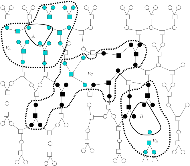
Figure 3: On the LDGM graph, $\mathcal{B}$ is depicted by the dark squares. The set $G\subseteq\mathcal{B}^{c}$ is depicted by the light squares. $A$ and $B$ contain both three nodes; there does not exist a self-avoiding walk that connects these two sets with all its check nodes in $G$. The sets of variable nodes $V_{A}$, $V_{B}$ and $V_{C}$ are disjoint as well as the sets of check nodes $G_{A}$, $G_{B}$ and $G_{C}$: these sets are enclosed in the dotted areas.

Now we examine a term of (106) for a $G$ that does not connect $A$ and $B$. Expanding the product $f_{A}f_{B}$, using linearity of the bracket and symmetry under exchange of replicas $(1)\leftrightarrow(2)$, it is equal to the difference $I-II$ where

$$I=\frac{1}{2Z^{\prime 2}}\sum_{u^{(1)},u^{(2)}}u^{(1)}_{A}u^{(1)}_{B}\prod_{i\in\mathcal{B}}e^{l_{i}(u_{\partial i}^{(1)}+u_{\partial i}^{(2)})+2|l_{i}|}\prod_{i\in G}K_{i}$$ (113)

$$II=\frac{1}{2Z^{\prime 2}}\sum_{u^{(1)},u^{(2)}}u^{(1)}_{A}u^{(2)}_{B}\prod_{i\in\mathcal{B}}e^{l_{i}(u_{\partial i}^{(1)}+u_{\partial i}^{(2)})+2|l_{i}|}\prod_{i\in G}K_{i}$$ (114)

Because of the disjointness of the sets $V_{A,B,C}$ and $C_{A,B,C}$ (the areas enclosed in dotted lines, see figure (3)) one can, in $I$ and $II$, factor the sums $\sum_{u^{(1)},u^{(2)}}$ in a product of three terms (in fact there is a fourth trivial term which is a power of $2$ coming from the bits outside the dotted areas). Then by symmetry $1\leftrightarrow 2$ one recognizes that $I=II$. Thus $I-II$ and this proves that $G$ does not contribute to (106) when it does not connect $A$ and $B$.

A.2 Cluster expansion for LDPC codes

Here we adapt the Berretti cluster expansion to our setting. For more details we refer to [21], [19]. Consider the replicated partition function

$$Z_{\perp}^{2} =\sum_{u^{(1)},u^{(2)}\in\{-1,+1\}^{m}}\prod_{k=1}^{n}(1+\tau^{(1)}_{k}e^{-2l_{k}})(1+\tau^{(2)}_{k}e^{-2l_{k}})$$ (115)

here $u^{(1)}=u^{(1)}_{1},\dots,u^{(1)}_{m};u^{(2)}=u^{(2)}_{1},\dots,u^{(2)}_{m}$ are two replicas of the information bits and $\tau^{(1)}_{k}=\prod_{a\in k}u^{(1)}_{a},\tau^{(2)}_{k}=\prod_{a\in k}u^{(2)}_{a}$. We have

$$\langle\tau_{i}\tau_{j}\rangle_{\perp}-\langle\tau_{i}\rangle_{\perp}\langle\tau_{j}\rangle_{\perp} =\frac{1}{2}\langle(\tau^{(1)}_{i}-\tau^{(2)}_{i})(\tau^{(1)}_{j}-\tau^{(2)}_{j})\rangle_{\perp,12}$$ (116)

where $\langle\cdot\rangle_{\perp,12}$ corresponds to the replicated system. We denote $f_{i}=\tau^{(1)}_{i}-\tau^{(2)}_{i}$, $f_{j}=\tau^{(1)}_{j}-\tau^{(2)}_{j}$. Then we have

$$\langle f_{i}f_{j}\rangle_{\perp,12}=\frac{1}{Z_{\perp}^{2}}\sum_{u^{(1)},u^{(2)}} f_{i}f_{j}\prod_{k}(1+E_{k})$$ (117)

where $E_{i}$ is defined in (60). Expanding the product we get,

$$\langle f_{i}f_{j}\rangle_{\perp,12} =\frac{1}{Z_{\perp}^{2}}\sum_{u^{(1)},u^{(2)}}f_{i}f_{j}\sum_{V\subset{\mathfrak{V}}}\prod_{k\in V}E_{k}$$

$$=\frac{1}{Z_{\perp}^{2}}\sum_{V\subset{\mathfrak{V}}}\sum_{u^{(1)},u^{(2)}}f_{i}f_{j}\prod_{k\in V}E_{k}$$ (118)

where ${\mathfrak{V}}$ denotes the set of all variable nodes of the original Tanner graph for the LDPC code and $V$ is any subset of distinct variable nodes. Suppose $V\subset{\mathfrak{V}}$ is such that one cannot create a walk (i.e. on the original Tannger graph of the LDPC code, a set of alternating variable and check nodes) connecting any check node in $\partial i$, to any check node in $\partial j$, and which has all its variable nodes contained entirely in $V$. Then we can partition $V$ into three mutually disjoint sets of variable nodes, $V_{1},V_{2},V_{3}$ such that $V_{1}\ni i$, $V_{2}\ni j$ and $V_{3}=V\setminus(V_{1}\cup V_{2})$. Note also that $\partial V_{1},\partial V_{2},\partial V_{3}$ are mutually disjoint otherwise we can create a walk between $\partial i$ and $\partial j$. Thus we can write

$$\sum_{u^{(1)},u^{(2)}}f_{i}f_{j}\prod_{k\in V}E_{k}=\sum_{\begin{subarray}{c}u^{(1)},u^{(2)}\\ u^{(1)}_{a},u^{(2)}_{a}\in\partial V_{1}\end{subarray}}f_{i}\prod_{k\in V_{1}}E_{k} \sum_{\begin{subarray}{c}u^{(1)},u^{(2)}\\ u^{(1)}_{a},u^{(2)}_{a}\in\partial V_{2}\end{subarray}}f_{j}\prod_{k\in V_{2}}E_{k}$$

$$\times\sum_{\begin{subarray}{c}u^{(1)},u^{(2)}\\ u^{(1)}_{a},u^{(2)}_{a}\in\partial V_{3}\end{subarray}}\prod_{k\in V_{3}}E_{k}$$ (119)

This implies that (119) vanishes. This is seen by using the antisymmetry of $f_{i}$ (or $f_{j}$) and the symmetry of $E_{k}$, under the exchange $(1)\leftrightarrow(2)$. Thus only those $V$ which contain a walk with all its variable nodes in $V$ and which intersects both $\partial i$ and $\partial j$ contributes to the sum in (A.2).

For any given $V$ (contributing to the sum) we construct the set of variable nodes $\Gamma_{V}$ as follows. $\Gamma_{V}$ is the union of all maximal connected clusters of distinct variable nodes in $V$, such that each of those connected clusters intersects $\partial i\cup\partial j$. Let $\Gamma_{V}^{c}=V\setminus\Gamma_{V}$. Clearly, there exists such a set because we know that the walk which connects $\partial i$ and $\partial j$ is a subset of $\Gamma_{V}$. Let $\hat{X}_{V}=\partial\Gamma_{V}\cup\partial i\cup\partial j$ be a set of check nodes. It is not difficult to see that $\hat{X}_{V}$ satisfies all the requirements of the set $\hat{X}$ in the sum (58). Indeed, consider $X_{V}=\Gamma_{V}\cup i\cup j$. By construction $\partial X_{V}=\hat{X}_{V}$; any two variable nodes in $X_{V}$ are connected by a walk with all its variable nodes in $X_{V}$; $\hat{X}_{V}$ contains both $\partial i$ and $\partial j$. Also note that $\Gamma_{V}$ is compatible with $\hat{X}_{V}$ as is required in the sum (59). Indeed, by construction $\partial\Gamma_{V}\cup\partial i\cup\partial j=\hat{X}_{V}$; $\partial\Gamma_{V}\cap\partial i\neq\phi$ and $\partial\Gamma_{V}\cap\partial j\neq\phi$; there exists a walk between $\partial i$ and $\partial j$ with all its variable nodes in $\Gamma_{V}$.

With this we can write

$$\langle f_{i}f_{j}\rangle_{\perp,12} =\frac{1}{Z_{\perp}^{2}}\sum_{V\subset{\mathfrak{V}}}\Big{\{}\sum_{\begin{subarray}{c}u_{a}^{(1)},u^{(2)}_{a}\\ a\in\partial\Gamma_{V}\cup\partial i\cup\partial j\end{subarray}}f_{i}f_{j}\prod_{k\in\Gamma_{V}}E_{k}\Big{\}}\Big{\{}\sum_{\begin{subarray}{c}u_{a}^{(1)},u_{a}^{(2)}\\ \text{remaining}\;a\end{subarray}}\prod_{k\in\Gamma_{V}^{c}}E_{k}\Big{\}}$$

$$=\frac{1}{Z_{\perp}^{2}}\sum_{\hat{X}}\sum_{\begin{subarray}{c}V\subset{\mathfrak{V}}\;:\\ \hat{X}_{V}=\hat{X}\end{subarray}}\Big{\{}\sum_{\begin{subarray}{c}u_{a}^{(1)},u^{(2)}_{a}\\ a\in\hat{X}\end{subarray}}f_{i}f_{j}\prod_{k\in\Gamma_{V}}E_{k}\Big{\}}\Big{\{}\sum_{\begin{subarray}{c}u_{a}^{(1)},u_{a}^{(2)}\\ \text{remaining}\;a\end{subarray}}\prod_{k\in\Gamma_{V}^{c}}E_{k}\Big{\}}$$ (120)

Now we resum over the sets $V$ such that $\hat{X}_{V}=\hat{X}$. These consist of $\Gamma$ compatible with $\hat{X}$ and the rest $\mathcal{G}$ which does not intersect $\hat{X}$. So

$$\langle f_{i}f_{j}\rangle_{\perp,12} =\frac{1}{Z_{\perp}^{2}}\sum_{\hat{X}}\Bigg{\{}\sum_{\begin{subarray}{c}u^{(1)}_{a},u^{(2)}_{a}\\ a\in\hat{X}\end{subarray}}\sum_{\begin{subarray}{c}\Gamma\text{compatible}\\ \text{with}\hat{X}\end{subarray}}f_{i}f_{j}\prod_{k\in\Gamma}E_{k}\Bigg{\}}\Bigg{\{}\sum_{\begin{subarray}{c}u^{(1)}_{a},u^{(2)}_{a}\\ a\in\hat{X}^{c}\end{subarray}}\sum_{\begin{subarray}{c}\mathcal{G}\subseteq{\mathfrak{V}}\\ \partial\mathcal{G}\cap\hat{X}=\phi\end{subarray}}\prod_{k\in\mathcal{G}}E_{k}\Bigg{\}}$$

$$=\frac{1}{Z_{\perp}^{2}}\sum_{\hat{X}}\Bigg{\{}\sum_{\begin{subarray}{c}u^{(1)}_{a},u^{(2)}_{a}\\ a\in\hat{X}\end{subarray}}\sum_{\begin{subarray}{c}\Gamma\text{compatible}\\ \text{with}\hat{X}\end{subarray}}f_{i}f_{j}\prod_{k\in\Gamma}E_{k}\Bigg{\}}\Bigg{\{}\sum_{\begin{subarray}{c}u^{(1)}_{a},u^{(2)}_{a}\\ a\in\hat{X}^{c}\end{subarray}}\prod_{\begin{subarray}{c}\text{all}\;k\;\text{s.t.}\\ \partial k\cap\hat{X}=\phi\end{subarray}}(1+E_{k})\Bigg{\}}$$ (121)

The last bracket is equal to (61) and we recognize Berretti’s expansion. Figure (4) shows a sample set $V$ and $\Gamma_{V}$ which give a non-vanishing contribution.

Figure 4: The dark variable nodes form the set $V=\{v_{1},\dots,v_{16}\}$. The walk $a_{1}v_{12}a_{2}v_{2}a_{3}v_{3}a_{4}v_{6}a_{5}v_{9}a_{6}v_{11}a_{7}$ connects $\partial i$ to $\partial j$ and hence this $V$ has a non-vanishing contribution. $\Gamma_{V}=\{v_{1},\dots,v_{12}\}$, is union of the two maximal connected clusters $\{v_{1},v_{13}\}$ and $\{v_{12},v_{2},v_{3},v_{4},v_{5},v_{6},v_{7},v_{8},v_{9},v_{10},v_{11}\}$ which has intersection with $\partial i\cup\partial j$. $\Gamma_{V}^{c}=\{v_{14},v_{15},v_{16}\}$.

References

- [1] T. Richardson, R. Urbanke “Modern Coding Theory,” Cambridge University Press 2008.
- [2] T. Richardson, R. Urbanke, “The Capacity of LDPC codes under Message-Passing Decoding,” IEEE Trans. Inf. Theory., pp. 638–656, 2001.
- [3] A. Montanari, “Tight Bounds for LDPC and LDGM Codes Under MAP Decoding,” IEEE Trans. Inf. Theory., 51, no. 9, pp. 3221–3246, (2005).
- [4] S. Kudekar, N. Macris, ”Sharp Bounds for MAP Decoding of General Irregular LDPC Codes”, Proc ISIT, Seattle, pp. 2259-2263 (2006)
- [5] F. Guerra, F. Toninelli, “Quadratic Replica Coupling in the Sherrington-Kirkpatrick Mean Field Spin Glass Model”, J. Math. Phys. 43 p. 3704 (2002).
- [6] C. Measson, A. Montanari, R. Urbanke, “Maxwell Construction: The Hidden Bridge between Iterative and Maximum a Posteriori Decoding”. Submitted to IEEE Transactions on Information Theory.
- [7] C. Measson, A. Montanari, T. Ridcharson, R. Urbanke, “The Generalized Area Theorem and Some of its Consequences”. Submitted to IEEE Transactions on Information Theory.
- [8] S. Franz, M. Leone, “Replica Bounds for Optimization Problems and Diluted Spin Systems,” J. Stat. Phys., 111 p. 535-564 (2003).
- [9] M. Talagrand; “Spin glasses: a Challenge for Mathematicians” Spinger-Verlag (2003)
- [10] S. Kudekar, S. Korada, N. Macris, ”Exact solution for the conditional entropy of Poissonian LDPC codes over the binary erasure channel”, ISIT pp. 1016-1021 (Nice 2007)
- [11] C. Méasson, A. Montanari, R. Urbanke, ”Asymptotic rate versus design rate”, ISIT pp. 1541-1545 (Nice 2007)
- [12] H. O. Georgii, ”Gibbs measures and phase transitions”, de Gruyter Studies in Mathematics 9 (1988).
- [13] N. Macris, ”Sharp Bounds on Generalized EXIT functions”, IEEE Trans. Inf. Theory., 53, No. 7, pp. 2365-2375 (2007).
- [14] N. Macris, “Griffith-Kelly-Sherman Correlation Inequalities: A Useful Tool in the Theory of Error Correcting Codes,” IEEE Trans. Inf. Theory. vol 53 p. 664-683 (2007).
- [15] S. Korada, R. Urbanke, “Exchange of Limits: Why Iterative Decoding Works”. Submitted to IEEE Transactions on Information Theory.
- [16] D. Brydges, “A Short Course on Cluster Expansions”, in Les Houches session XLIII (1984).
- [17] S. Kudekar, N. Macris, “Proof of replica formulas in the high noise regime for communication using LDGM codes”, Information Theory Workshop, pp. 416-4120 (Porto 2008)
- [18] S. Kudekar, N. Macris, “Decay of Correlations in Low Density Parity Check Codes: Low Noise Regime”. Submitted to International Symposium on Information Theory, Seoul 2009.
- [19] J. Fröhlich, ”Mathematical aspects of disordered systems”, in Les Houches session XLIII (1984).
- [20] H. Dreifus, A. Klein, J. Perez, “Taming Griffiths’ singularities: Infinite differentiability of quenched correlation functions,” Communications in Mathematical Physics, 170, pp.21-39.
- [21] A. Berretti, ”Some properties of random Ising models”, Journal of statistical physics, vol 38 pp. 483-496 (1985)
- [22] S. Tatikonda and M. I. Jordan, “Loopy Belief Propagation and Gibbs Measures”, 18th Conference on Uncertainty in Artificial Intelligence, August 2002 (Edmonton, Canada).
- [23] T. Murayama, Y. Kabashima, D. Saad, R. Vicente, “The Statistical Physics of Regular Low-Density Parity-Check Error-Correcting Codes”. Phys. Rev. E 62(2) 1577-1591 (2000).
- [24] D. Forney, “Codes on graphs: normal realizations”. IEEE Transactions on Information Theory, vol 47 pp. 520-548 (2001).
- [25] A. Ashikmin, G. Kramer, S. ten Brink, ”Extrinsic information transfer functions: model and erasure channel property” IEEE Trans. Inform. Theory, vol 50, pp. 2657-2673 (2004)
- [26] S. Kudekar, N. Macris, ”Decay of correlations: an application to low density parity check codes”, 5th International Symp osium on Turbo Codes and Related Topics, pp. 13-18 (Lausanne 2008)
- [27] A. Montanari, D. Shah, “Counting Good Truth Assignmants for Random Satisfiability Formulae”. Proceedings of Symposium of Discrete Algorithms (SODA), New Orleans, September 2007.
- [28] M. Chertkov, V. Chernyak, “Loop series for discrete statistical models on graphs”, JSTAT (2006) P06009.
- [29] A. Procacci1, B. Scoppola, “Statistical Mechanics Approach to Coding Theory”.Journal of Statistical Physics, vol 96, pp 907-912, 1999.