Weak localization in monolayer and bilayer graphene

Abstract

We describe the weak localization correction to conductivity in ultra-thin graphene films, taking into account disorder scattering and the influence of trigonal warping of the Fermi surface. A possible manifestation of the chiral nature of electrons in the localization properties is hampered by trigonal warping, resulting in a suppression of the weak anti-localization effect in monolayer graphene and of weak localization in bilayer graphene. Intervalley scattering due to atomically sharp scatterers in a realistic graphene sheet or by edges in a narrow wire tends to restore weak localization resulting in negative magnetoresistance in both materials.

1 Introduction

The chiral nature of quasiparticles in ultra-thin graphitic films DiVincenzo ; Semenoff ; haldane88 ; AndoNoBS ; McCann recently revealed in Shubnikov de Haas and quantum Hall effect measurements NovScience ; Novoselov ; Zhang ; QHEbi originates from the hexagonal lattice structure of a monolayer of graphite (graphene). The low energy behavior of monolayer graphene is explained in terms of two valleys of Dirac-like chiral quasiparticles with ‘isospin’ linked to the momentum direction, exhibiting Berry phase $\pi$ DiVincenzo ; Semenoff ; haldane88 ; AndoNoBS . Remarkably, the dominant low energy quasiparticles in a bilayer are different: massive chiral quasiparticles with a parabolic dispersion and Berry phase $2\pi$ McCann .

In existing graphene structures, scattering occurs predominantly from potential perturbations which are smooth on the scale of the lattice constant $a$. This smooth potential arises from charges located in the substrate at a distance $d$ from the 2D sheet, $a\ll d<h/p_{F}$ ($h/p_{\mathrm{F}}$ being the Fermi wavelength). Such a smooth potential is unable to change the isospin of chiral electrons so that, in a monolayer, there is a complete suppression of electron backscattering from potential disorder AndoNoBS ; AndoWL . In the theory of quantum transport in disordered systems WL the suppression of backscattering is known as the anti-localization (WAL) effect WLso and, in monolayer graphene with purely potential scattering, a possible WAL behavior of conductivity AndoWL ; khve06 ; guinea06 ; WLmono has been related to the Berry phase $\pi$ specific to the Dirac-like Hamiltonian. Owing to the different degree of chirality in bilayer graphene, related to Berry phase $2\pi$ McCann , purely potential scattering would have a different effect: no suppression of backscattering leading to conventional weak localization (WL) guinea06 ; WLbilayer .

In realistic graphene, there are other considerations that appear, at first glance, to be merely small perturbations to this picture, but they have a profound impact on the localization properties if their effect is perceptible on length scales less than the phase coherence length. This includes influence of ripples on the graphene sheet WLman leading to a weak randomization of carbon $\pi$-bands, scattering off short-range defects that do not conserve isospin and valley AndoWL ; khve06 ; guinea06 ; WLmono , and trigonal warping of the electronic band structure which introduces asymmetry in the shape of the Fermi surface about each valley AndoNoBS ; WLmono ; WLbilayer . Both of them tend to destroy the manifestation of chirality in the localization properties, resulting in a suppression of the WAL effect in monolayer graphene WLman and of WL in bilayers exeter . Moreover, owing to the inverted chirality of quasiparticles in the two valleys, intervalley scattering will wash out any Berry phase effect and restore conventional weak localization (WL) behavior of electrons in both monolayers and bilayers in the regime of long-lasting phase coherence AndoWL ; khve06 ; guinea06 ; WLmono ; WLbilayer ; WLman ; exeter ; berger .

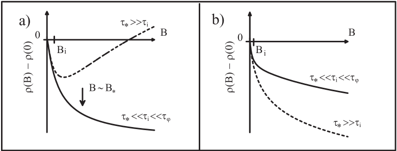
Figure 1: ($\mathbf{a}$) Typical magnetoresistance behavior expected in a phase-coherent ($\tau_{\varphi}\gg\tau_{i}$) monolayer of graphene for a weak intervalley scattering, $\tau_{\ast}\ll\tau_{i}$ (solid line) and for the case when the symmetry-breaking intravalley scattering is slower than the intervalley one $\tau_{\ast}\gg\tau_{i}$ (dashed). In both cases, we assume that the phase coherence time determines the longest relaxation time scale in the system. ($\mathbf{b}$) Magnetoresistance of bilayer graphene, $\tau_{\ast}\ll\tau_{i}$ (solid line) and $\tau_{\ast}\gg\tau_{i}$ (dashed). Note that, for the case when $\tau_{\varphi}\ll\tau_{i}$ and $\tau_{\ast}\ll\tau_{i},\Delta\rho(B)=0$ in both monolayer and bilayer graphene.

Two typical magnetoresistance curves for monolayer graphene are sketched in figure 1(a). They illustrate two extremes: $\tau_{\ast}\gg\tau_{\mathrm{i}}$ and $\tau_{\ast}\ll\tau_{\mathrm{i}}$ where $\tau_{\mathrm{i}}$ is the intervalley scattering time and $\tau_{\ast}$ is the combined scattering time of intravalley and intervalley scattering and of trigonal warping (see equation (15,16) and (3.3) below). When $\tau_{\ast}\gg\tau_{\mathrm{i}}$, the magnetoresistance $\rho(B)-\rho(0)$ changes sign at the field $B_{i}$ such that $\tau_{B}\sim\tau_{\mathrm{i}}$: from negative at $B<B_{i}$ to positive at higher fields. This behavior resembles the low-to-high field crossover in the quantum correction to the conductivity of metals with strong spin-orbit coupling, though with an inverted sign of the effect. In the case of $\tau_{\ast}\ll\tau_{\mathrm{i}}$, the magnetoresistance is typically of a WL type, with almost no sign of anti-localization up to the highest fields, which shows that, unlike in a ballistic regime or a quantizing magnetic field haldane88 ; McCann ; CheianovFalko , the chiral nature of quasiparticles does not manifest itself in the weak field magnetoresistance of realistic graphene structures. In bilayer, however, slight enhancement of WL behavior is expected in the case of weak intravalley symmetry breaking scattering, $\tau_{\ast}\ll\tau_{\mathrm{i}}$, due to different Berry phase $2\pi$. In the case of very strong intravalley symmetry breaking scattering, $\tau_{\ast}\gg\tau_{\mathrm{i}}$ conventional WL magnetoresistance is expected.

The WL behavior in graphene is novel because, with the exception of spin-orbit coupling WLso ; dresselhaus92 , qualitative features of WL do not usually depend on the detail of the electronic band structure and crystalline symmetry. In gapful multi-valley semiconductors only the size of WL effect may depend on the number of valleys and the strength of intervalley scattering fuku80 ; bishop80 ; prasad95 . The low-field MR, $\Delta\rho(B)\equiv\rho(B)-\rho(0)$, in a two dimensional electron gas or a thin metallic film WL ; WLso ; fuku80 ; socomment in the absence of spin-orbit coupling is characterized by

$$\Delta\rho(B) = -\frac{s_{\theta}e^{2}\rho^{2}}{2\pi h}F\left(\frac{B}{B_{\varphi}}\right),\;B_{\varphi}=\frac{\hbar c}{4De}\tau_{\varphi}^{-1}.$$ (1)

Here $F(z)=\ln z+\psi(\frac{1}{2}+\frac{1}{z})$, $\tau_{\varphi}$ is the coherence time, $D$ is the diffusion coefficient, and the integer factor $s_{\theta}$ depends on whether or not states in $n_{v}$ valleys are mixed by disorder. This factor is controlled by the ratio $\theta=\tau_{\mathrm{i}}/\tau_{\varphi}$ between the intervalley scattering time $\tau_{\mathrm{i}}$ and the coherence time $\tau_{\varphi}$. In materials such as Mg, ZnO, Si, Ge, listed in Table I, where each of the Fermi surface pockets is $\mathbf{p}\rightarrow-\mathbf{p}$ symmetric, intervalley scattering reduces the size of the WL MR from that described by $s_{\infty}=2n_{v}$ when $\theta=\tau_{\mathrm{i}}/\tau_{\varphi}\gg 1$ to $s_{0}=2$ for $\theta\ll 1$.

A more interesting scenario develops in a multi-valley semimetal, where the localization properties can be influenced by the absence of $\mathbf{p}\rightarrow-\mathbf{p}$ symmetry of the electronic dispersion within a single valley, and graphene is an example of such a system. Here, we demonstrate how the asymmetry in the shape of the Fermi surface in each of its two valleys determines the observable WL behavior sketched in figure 1(a,b). It has a tendency opposite to that known in usual semiconductors and metals: a complete absence of WL MR for infinite $\tau_{\mathrm{i}}$ ($s_{\infty}=0$) and the standard WL effect in the limit of $\tau_{\mathrm{i}}\,\ll\tau_{\varphi}$ ($s_{0}=2$). In Section 2 we describe the WL effect in monolayer graphene with a description of the low energy Hamiltonian in Section 2.1, a qualitative account of interference effects in Section 2.2, the model of disorder in Section 2.3, an account of our diagrammatic calculation of the weak localization correction in Section 2.4 and the resulting magnetoresistance in Section 2.5. Section 3 describes the weak localization correction and magnetoresistance in bilayer graphene.

Table 1: Weak localization factor $s_{\theta}$ in conductors with a multi-valley conduction band and negligible spin-orbit coupling. The factor $s_{\theta}$ is specified for two limiting cases, no inter-valley scattering $\theta=\tau_{\mathrm{i}}/\tau_{\varphi}\rightarrow\infty$, and for fast inter-valley scattering $\theta\rightarrow 0$.

$n_{v}$		$s_{\infty}$	$s_{0}$
$1$	Mg films bergmann84 , ZnO wells goldenblum99	$2$	-
$2,6$	Si MOSFETs fuku80 ; bishop80	$2n_{v}$	$2$
$2$	Si/SiGe wells prasad95	$4$	$2$
$2$	monolayer graphene	$0$	$2$
$2$	bilayer graphene	$0$	$2$

2 Weak localization magnetoresistance in disordered monolayer graphene

2.1 Low energy Hamiltonian of clean monolayer graphene

The hexagonal lattice of monolayer graphene contains two non-equivalent sites $A$ and $B$ in the unit cell, as shown in figure 2(a). The Fermi level in a neutral graphene sheet is pinned near the corners of the hexagonal Brillouin zone with wave vectors $\mathbf{K}_{\pm}=\pm({\textstyle\frac{2}{3}}ha^{-1},0)$ where $a$ is the lattice constant. The Brillouin zone corners $\mathbf{K}_{\pm}$ determine two non-equivalent valleys in the quasiparticle spectrum described by the Hamiltonian DiVincenzo ; AndoNoBS ; WLmono ; wallace ,

$${\hat{H}}_{1} = v\Pi_{z}\left(\sigma_{x}p_{x}+\sigma_{y}p_{y}\right)+{\hat{h}}_{1w},$$ (2)

$${\hat{h}}_{1w} = \mu\Pi_{0}\left[\sigma_{y}\left({p}_{x}{p}_{y}+{p}_{y}{p}_{x}\right)-\sigma_{x}\left({p}_{x}^{2}-{p}_{y}^{2}\right)\right].$$

This Hamiltonian operates in the space of four-component wave functions, $\Phi=[\phi_{\mathbf{K}_{+}}(A),\phi_{\mathbf{K}_{+}}(B),\\ \phi_{\mathbf{K}_{-}}(B),\phi_{\mathbf{K}_{-}}(A)]$ describing electronic amplitudes on $A$ and $B$ sites and in the valleys $\mathbf{K}_{\pm}$. Here, we use a direct product of ‘isospin’ ($AB$ lattice space) matrices $\sigma_{0}\equiv\hat{1},\sigma_{x,y,z}$ and ‘pseudospin’ inter/intra-valley matrices $\Pi_{0}\equiv\hat{1},\Pi_{x,y,z}$ to highlight the difference between the form of ${\hat{H}}_{1}$ in the non-equivalent valleys. The Hamiltonian ${\hat{H}}_{1}$ takes into account nearest neighbor $A/B$ hopping in the plane with the first (second) term representing the first (second) order term in an expansion with respect to momentum $\mathbf{p}$ measured from the center of the valley $\mathbf{K}_{\pm}$.

Near the center of the valley $\mathbf{K}_{+}$, the Dirac-type part, $v\,\mathbf{\sigma\cdot p}$, of ${\hat{H}}_{1}$ determines the linear dispersion $\epsilon=vp$ for the electron in the conduction band and $\epsilon=-vp$ for the valence band. Electrons in the conduction and valence band also differ by the isospin projection onto the direction of their momentum (chirality): $\mathbf{\sigma}\cdot\mathbf{p}/p=1$ in the conduction band, $\mathbf{\sigma}\cdot\mathbf{p}/p=-1$ in the valence band. In the valley $\mathbf{K}_{-}$, the electron chirality is mirror-reflected: it fixes $\mathbf{\sigma}\cdot\mathbf{p}/p=-1$ for the conduction band and $\mathbf{\sigma}\cdot\mathbf{p}/p=1$ for the valence band. For an electron in the conduction band, the plane wave state is

$$\Phi_{\mathbf{K}_{\pm},\mathbf{p}} = \frac{e^{i\mathbf{pr}/\hbar}}{\sqrt{2}}\left(\pm e^{-i\varphi/2}|\uparrow\rangle_{\mathbf{K}_{\pm},\mathbf{p}}+e^{i\varphi/2}|\downarrow\rangle_{\mathbf{K}_{\pm},\mathbf{p}}\right),$$ (3)

$$\Phi_{\mathbf{K}_{\pm},-\mathbf{p}} = \frac{ie^{-i\mathbf{pr}/\hbar}}{\sqrt{2}}\left(\mp e^{-i\varphi/2}|\uparrow\rangle_{\mathbf{K}_{\pm},-\mathbf{p}}+e^{i\varphi/2}|\downarrow\rangle_{\mathbf{K}_{\pm},-\mathbf{p}}\right).$$ (4)

Here ${|\uparrow\rangle_{\mathbf{K}_{+},\mathbf{p}}}=[1,0,0,0]$, ${|\downarrow\rangle_{\mathbf{K}_{+},\mathbf{p}}}=[0,1,0,0]$ and ${|\uparrow\rangle_{\mathbf{K}_{-},\mathbf{p}}}=[0,0,1,0]$, ${|\uparrow\rangle_{\mathbf{K}_{-},\mathbf{p}}}=[0,0,0,1]$, and the factors $e^{\pm i\varphi/2}$ take into account the chirality, with angle $\varphi$ defining the direction of momentum in the plane $\mathbf{p}=(p\cos\varphi,p\sin\varphi)$. The angular dependence $w(\varphi)\sim\cos^{2}(\varphi/2)$ of the scattering probability off a short range potential which conserves isospin is shown in figure 3(a). It demonstrates the fact that the chiral states Eqs. (3,4) with isospin fixed to the direction of momentum display an absence of back scattering AndoNoBS ; shon98 ; AndoWL , leading to a transport time longer than the scattering time $\tau_{\textrm{tr}}=2\tau_{0}$.

Figure 2: ($\mathbf{a}$)Schematic plan view of the monolayer lattice containing two sites in the unit cell, $A$ (white circles) and $B$ (grey), arranged on an hexagonal lattice (solid lines). ($\mathbf{b}$)Fermi lines (solid lines) in the vicinity of two inequivalent valleys $\mathbf{K}_{+}$ and $\mathbf{K}_{-}$ of the hexagonal Brillouin zone (dashed line). Trigonal warping produces asymmetry of the dispersion at each valley $\epsilon(\mathbf{K}_{\pm},\mathbf{p})\neq\epsilon(\mathbf{K}_{\pm},-\mathbf{p})$, where momentum $\mathbf{p}$ is determined with respect to the center of the valley, but the effects of warping in the valleys have opposite signs, $\epsilon(\mathbf{K}_{\pm},\mathbf{p})=\epsilon(\mathbf{K}_{\mp},-\mathbf{p})$.

The term ${\hat{h}}_{1\mathrm{w}}$ in equation (2) can be treated as a perturbation leading to a trigonal deformation of a single-connected Fermi line and $\mathbf{p}\rightarrow-\mathbf{p}$ asymmetry of the electron dispersion inside each valley illustrated in figure 2(b): $\epsilon(\mathbf{K}_{\pm},\mathbf{p})\neq\epsilon(\mathbf{K}_{\pm},-\mathbf{p})$. However, due to time-reversal symmetry t-rev trigonal warping has opposite signs in the two valleys and $\epsilon(\mathbf{K}_{\pm},\mathbf{p})=\epsilon(\mathbf{K}_{\mp},-\mathbf{p})$. The interplay between the two terms in ${\hat{H}}_{1}$ resulting in the asymmetry of the electronic dispersion manifest itself in the WL behavior.

2.2 Interference of electronic waves in monolayer graphene

The WL correction to conductivity in disordered conductors is a result of the constructive interference of electrons propagating around closed loops in opposite directions WL as sketched in figure 3(b). Such interference is constructive in metals and semiconductors with negligibly weak spin-orbit coupling, since electrons acquire exactly the same phase when travelling along two time-reversed trajectories.

WL is usually described WL in terms of the particle-particle correlation function, Cooperon. Following the example of Cooperons for a spin ${\textstyle\frac{1}{2}}$, we classify Cooperons as singlets and triplets in terms of ‘isospin’ ($AB$ lattice space) and ‘pseudospin’ (inter/intra-valley) indices (see Section 2.1). In fact, with regards to the isospin (sublattice) composition of Cooperons in a disordered monolayer, only singlet modes are relevant. This is because a correlator describing two plane waves, $\Phi_{\mathbf{K}_{+},\mathbf{p}}$ and $\Phi_{\mathbf{K}_{-},-\mathbf{p}}$ Eqs. (3,4), propagating in opposite directions along a ballistic segment of a closed trajectory as in figure 3(b) has the following form:

$$\Phi_{\mathbf{K},\mathbf{p}}\Phi_{\mathbf{K}^{\prime},-\mathbf{p}} \sim |\uparrow\rangle_{\mathbf{K},\mathbf{p}}|\downarrow\rangle_{\mathbf{K}^{\prime},-\mathbf{p}}-|\downarrow\rangle_{\mathbf{K},\mathbf{p}}|\uparrow\rangle_{\mathbf{K}^{\prime},-\mathbf{p}}-e^{-i\varphi}|\uparrow\rangle_{\mathbf{K},\mathbf{p}}|\uparrow\rangle_{\mathbf{K}^{\prime},-\mathbf{p}}+e^{i\varphi}|\downarrow\rangle_{\mathbf{K},\mathbf{p}}|\downarrow\rangle_{\mathbf{K}^{\prime},-\mathbf{p}}.$$

It contains only sublattice-singlet terms (the first two terms) because triplet terms (the last two terms) disappear after averaging over the direction of momentum, $\mathbf{p}=(p\cos\varphi,p\sin\varphi)$, so that $\langle e^{\pm i\varphi}\rangle_{\varphi}=0$. In fact, our diagrammatic calculation described in Section 2.4 shows that the interference correction to the conductivity of graphene is determined by the interplay of four isospin singlet modes: one pseudospin singlet and three pseudospin triplets. Of these, two of the pseudospin triplet modes are intravalley Cooperons while the remaining triplet and the singlet are intervalley Cooperons.

In the WL picture for a diffusive electron in a metal, two phases $\vartheta_{1}$ and $\vartheta_{2}$ acquired while propagating along paths $"1"$ and $"2"$ [see figure 3(b)] are exactly equal, so that the interference of such paths is constructive and, as a result, enhances backscattering leading to WL WL . In monolayer graphene the Berry phase $\pi$ characteristic for quasi-particles described by the first term of ${\hat{H}}_{1}$, determines the phase difference $\delta\equiv\vartheta_{1}-\vartheta_{2}=\pi N$ (where $N$ is the winding number of a trajectory) AndoWL ; WLmono , and one would expect weak anti-localization behavior. However, the asymmetry of the electron dispersion due to ${\hat{h}}_{\mathrm{1w}}$, leading to warping of the Fermi line around each valley as in figure 2(b), deviates $\delta$ from $\pi N$. Indeed, any closed trajectory is a combination of ballistic intervals, figure 3(b). Each interval, characterized by the momenta $\pm\mathbf{p_{j}}$ (for the two directions) and by its duration $t_{j}$, contributes to the phase difference $\delta_{j}=[\epsilon(\mathbf{p_{j}})-\epsilon(-\mathbf{p_{j}})]t_{j}={\hat{h}}_{\mathrm{1w}}(\mathbf{p_{j}})t_{j}$. Since $\delta_{j}$ are random uncorrelated, the mean square of $\delta=\sum\delta_{j}$ can be estimated as $\langle\delta^{2}\rangle\sim\langle(t_{j}{\hat{h}}_{\mathrm{1w}}(\mathbf{p_{j}}))^{2}\rangle t/\tau_{tr}$, where $t$ is the duration of the path and $\tau_{tr}$ is the transport mean free time. Warping thus determines the relaxation rate,

$$\tau_{\mathrm{w}}^{-1}\sim\langle\mathrm{Tr}{\hat{h}}_{\mathrm{1w}}^{2}(\mathbf{p})\rangle_{\varphi},$$ (5)

which suppresses the two intravalley Cooperons, and, thus, weak anti-localization in the case when electrons seldom change their valley state. The two intervalley Cooperons are not affected by trigonal warping due to time-reversal symmetry of the system which requires $\epsilon(\mathbf{K}_{\pm},\mathbf{p})=\epsilon(\mathbf{K}_{\mp},-\mathbf{p})$, figure 2(b). These two Cooperons cancel each other in the case of weak intervalley scattering, thus giving $\delta g\sim 0$. However, intervalley scattering, with a rate $\tau_{\mathrm{i}}^{-1}$ larger than the decoherence rate $\tau_{\varphi}^{-1}$, breaks the exact cancellation of the two intervalley Cooperons and partially restores weak localization.

2.3 Matrix parameterization, valley symmetry and the model of disorder

To describe the valley symmetry of monolayer graphene and parameterize all possible types of disorder, we introduce two sets of 4$\times$4 Hermitian matrices $\vec{\Sigma}=(\Sigma_{x},\Sigma_{y},\Sigma_{z})$ with $[\Sigma_{s_{1}},\Sigma_{s_{2}}]=2i\varepsilon^{s_{1}s_{2}s_{3}}\Sigma_{s_{3}}$, and ’pseudospin’ $\vec{\Lambda}=(\Lambda_{x},\Lambda_{y},\Lambda_{z})$ with $[\Lambda_{l_{1}},\Lambda_{l_{2}}]=2i\varepsilon^{l_{1}l_{2}l_{3}}\Sigma_{l_{3}}$, defined as

$$\Sigma_{x} = \Pi_{z}\otimes\sigma_{x},\;\Sigma_{y}=\Pi_{z}\otimes\sigma_{y},\;\Sigma_{z}=\Pi_{0}\otimes\sigma_{z},$$ (6)

$$\Lambda_{x} = \Pi_{x}\otimes\sigma_{z},\;\Lambda_{y}=\Pi_{y}\otimes\sigma_{z},\;\Lambda_{z}=\Pi_{z}\otimes\sigma_{0}.$$ (7)

The operators $\vec{\Sigma}$ and $\vec{\Lambda}$ form two mutually independent algebras equivalent to the algebra of Pauli matrices (in Eqs. (6,7) $\varepsilon^{s_{1}s_{2}s_{3}}$ is the antisymmetric tensor and $[\Sigma_{s},\Lambda_{l}]=0$) thus they determine two commuting subgroups of the group U₄ of unitary transformations U4 of a 4-component $\Phi$: an ’isospin’ sublattice group SU${}_{2}^{\Sigma}\equiv\{e^{ia\vec{n}\cdot\!\vec{\Sigma}}\}$ and a ’pseudospin’ valley group SU${}_{2}^{\Lambda}\equiv\{\mathrm{e}^{ib\vec{n}\cdot\!\vec{\Lambda}}\}$. Also, $\vec{\Sigma}$ and $\vec{\Lambda}$ change sign under the inversion of time, whereas products $\Sigma_{s}\Lambda_{l}$ are invariant with respect to the $t\rightarrow-t$ transformation and can be used as a basis for a quantitative phenomenological description of non-magnetic static disorder shon98 ; mf05 . Table 1 is a summary of the discrete symmetries of the operators $\vec{\Sigma}$ and $\vec{\Lambda}$ and their products $\Sigma_{s}\Lambda_{l}$. Time reversal $T$ of an operator $\hat{W}$ is described by $(\Pi_{x}\otimes\sigma_{x}){\hat{W}}^{\ast}(\Pi_{x}\otimes\sigma_{x})$. The rotation by $\pi/3$ about the perpendicular $z$ axis is described by $C_{6}=\Pi_{x}\otimes\exp[(-2\pi i/3)\sigma_{z}]$. Reflection in the $x$-$z$ plane is $R_{x}=\Pi_{0}\otimes\sigma_{x}$.

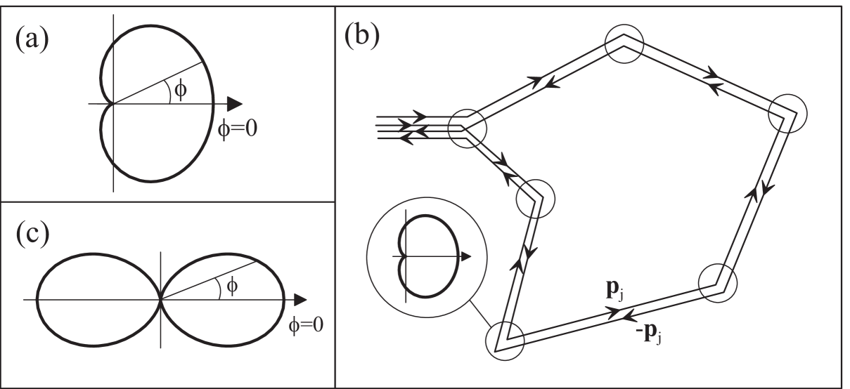
Figure 3: (a) angular dependence $w(\varphi)\sim\cos^{2}(\varphi/2)$ of the scattering probability off a short range potential in monolayer graphene, (b) a pair of closed paths which contribute to weak localization, (c) angular dependence $w(\varphi)\sim\cos^{2}(\varphi)$ of the scattering probability off a short range potential in bilayer graphene.

The operators $\vec{\Sigma}$ and $\vec{\Lambda}$ help us to represent the electron Hamiltonian in weakly disordered graphene as

$${\hat{H}_{1}}=v\,\vec{\Sigma}\mathbf{p}+{\hat{h}}_{\mathrm{1w}}+\mathrm{\hat{I}}u(\mathbf{r})+\sum_{s,l=x,y,x}\Sigma_{s}\Lambda_{l}u_{s,l}(\mathbf{r}),$$ (8)

$$\mathrm{where}\;\;{\hat{h}}_{\mathrm{1w}}=-\mu\Sigma_{x}(\,\vec{\Sigma}\mathbf{p})\Lambda_{z}\Sigma_{x}(\,\vec{\Sigma}\mathbf{p})\Sigma_{x}.$$

The Dirac-type part $v\,\vec{\Sigma}\mathbf{p}$ of ${\hat{H}_{1}}$ in equation (8) and potential disorder $\mathrm{\hat{I}}u(\mathbf{r})$ (where $\mathrm{\hat{I}}$ is a 4$\times$4 unit matrix and $\left\langle u\left(\mathbf{r}\right)u\left(\mathbf{r}^{\prime}\right)\right\rangle=u^{2}\delta\left(\mathbf{r}-\mathbf{r}^{\prime}\right)$) do not contain valley operators $\mathbf{\Lambda}_{l}$, thus, they remain invariant with respect to the pseudospin transformations from valley group SU${}_{2}^{\Lambda}$. Below, we assume that the isospin/pseudospin-conserving disorder due to charges lying in a substrate at distances from the graphene sheet shorter or comparable to the electron wavelength $h/p_{\mathrm{F}}$ dominates the elastic scattering rate, $\tau^{-1}\approx\tau_{0}^{-1}=\pi\gamma u^{2}/\hbar$, where $\gamma=p_{\mathrm{F}}/(2\pi\hbar^{2}v)$ is the density of states of quasiparticles per spin in one valley. All other types of disorder which originate from atomically sharp defects shon98 ; mf05 and break the SU${}_{2}^{\Lambda}$ pseudospin symmetry of the system are included in a random matrix $\Sigma_{s}\Lambda_{l}u_{s,l}(\mathbf{r})$. In particular, $u_{z,z}(\mathbf{r})$ describes disorder due to different on-site energies on the $A$ and $B$ sublattices, $u_{x(y),z}(\mathbf{r})$ plays the role of a valley-antisymmetric vector potential of a geometrical nature, and $u_{s,x(y)}(\mathbf{r})$ take into account inter-valley scattering. For simplicity, we assume that different types of disorder are uncorrelated, $\langle u_{s,l}(\mathbf{r})u_{s^{\prime},l^{\prime}}(\mathbf{r}^{\prime})\rangle=u_{sl}^{2}\delta_{ss^{\prime}}\delta_{ll^{\prime}}\delta(\mathbf{r}-\mathbf{r}^{\prime})$ and, on average, isotropic in the $x-y$ plane, $u_{xl}^{2}=u_{yl}^{2}\equiv u_{\bot l}^{2}$, $u_{sx}^{2}=u_{sy}^{2}\equiv u_{s\bot}^{2}$. We parametrize them by scattering rates $\tau_{sl}^{-1}=\pi\gamma u_{sl}^{2}/\hbar$. Also, the warping term, ${\hat{h}}_{\mathrm{1w}}$ lifts the pseudospin symmetry SU${}_{2}^{\Lambda}$, though it remains invariant under pseudospin rotations around the z-axis.

To characterize Cooperons in monolayer graphene, we use a Cooperon matrix $C_{\alpha\beta\alpha^{\prime}\beta^{\prime}}^{\xi\mu\xi^{\prime}\mu^{\prime}}$ where subscripts describe the isospin state of incoming $\alpha\beta$ and outgoing $\alpha^{\prime}\beta^{\prime}$ pairs of electrons and superscripts describe the pseudospin state of incoming $\xi\mu$ and outgoing $\xi^{\prime}\mu^{\prime}$ pairs. Following the example of Cooperons for a spin ${\textstyle\frac{1}{2}}$, we classify Cooperons as singlets and triplets in terms of isospin and pseudospin indices $C_{S_{1}S_{2}}^{M_{1}M_{2}}$. For example, $M=0$ is a ‘pseudospin-singlet’, $M=x,y,z$ are three ‘pseudospin-triplet’ components; $S=0$ is a ‘isospin-singlet’ and $S=x,y,z$ are ‘pseudospin-triplet’ components. It is convenient to use pseudospin as a quantum number to classify the Cooperons in graphene because of the hidden SU${}_{2}^{\Lambda}$ symmetry of the dominant part of the free-electron and disorder Hamiltonian.

Table 2: Matrices ${\Sigma}_{s}$ and ${\Lambda}_{l}$ provide us with representations of the crystalline symmetry group, which is constructed of $3$ generators, ${\textstyle\frac{\pi}{3}}$-rotation, $C_{6}$, mirror reflection with respect to $Ox$ axis, $R_{x}$, and translation along $Ox$ by lattice constant, $\mathbf{a}$. Operation $T$ stands for the time reversal, $t\rightarrow-t$. Here, ${\Sigma}_{s}$ and ${\Lambda}_{l}$ are grouped into bases forming irreducible representations which can be $1,2$ and 4 dimensional. The transformation matrixes $U_{ji}$, $g\phi_{i}=\sum_{j}U_{ji}(g)\phi_{j}$ ($g$ stands for a symmetry operation), are given explicitly for each of such bases $\phi_{i}$.

$\Sigma_{s}\Lambda_{l}$	$T$	$C_{6}$	$R_{x}$	$\mathbf{a}$
$\hat{I}$	$+1$	$+1$	$+1$	$+1$
$\Sigma_{z}$	$-1$	$+1$	$-1$	$+1$
$\Lambda_{z}$	$-1$	$-1$	$+1$	$+1$
$\Sigma_{z}\Lambda_{z}$	$+1$	$-1$	$-1$	$+1$
$\left[\begin{array}[]{cc}\Sigma_{x}&\\ \Sigma_{y}&\\ \end{array}\right]$	$-1$	$\left(\begin{array}[]{cc}\frac{1}{2}&\frac{\sqrt{3}}{2}\\ -\frac{\sqrt{3}}{2}&\frac{1}{2}\\ \end{array}\right)$	$\left(\begin{array}[]{cc}1&0\\ 0&-1\\ \end{array}\right)$	$\left(\begin{array}[]{cc}1&0\\ 0&1\\ \end{array}\right)$
$\left[\begin{array}[]{cc}\Lambda_{x}\\ \Lambda_{y}\\ \end{array}\right]$	$-1$	$\left(\begin{array}[]{cc}1&0\\ 0&-1\\ \end{array}\right)$	$\left(\begin{array}[]{cc}-1&0\\ 0&-1\\ \end{array}\right)$	$\left(\begin{array}[]{cc}-\frac{1}{2}&-\frac{\sqrt{3}}{2}\\ \frac{\sqrt{3}}{2}&-\frac{1}{2}\\ \end{array}\right)$
$\left[\begin{array}[]{cc}\Lambda_{z}\Sigma_{x}\\ \Lambda_{z}\Sigma_{y}\\ \end{array}\right]$	$+1$	$\left(\begin{array}[]{cc}-\frac{1}{2}&-\frac{\sqrt{3}}{2}\\ \frac{\sqrt{3}}{2}&-\frac{1}{2}\\ \end{array}\right)$	$\left(\begin{array}[]{cc}1&0\\ 0&-1\\ \end{array}\right)$	$\left(\begin{array}[]{cc}1&0\\ 0&1\\ \end{array}\right)$
$\left[\begin{array}[]{cc}\Lambda_{x}\Sigma_{z}\\ \Lambda_{y}\Sigma_{z}\\ \end{array}\right]$	$+1$	$\left(\begin{array}[]{cc}1&0\\ 0&-1\\ \end{array}\right)$	$\left(\begin{array}[]{cc}1&0\\ 0&1\\ \end{array}\right)$	$\left(\begin{array}[]{cc}-\frac{1}{2}&-\frac{\sqrt{3}}{2}\\ \frac{\sqrt{3}}{2}&-\frac{1}{2}\\ \end{array}\right)$
$\left[\begin{array}[]{cccc}\Lambda_{x}\Sigma_{x}\\ \Lambda_{x}\Sigma_{y}\\ \Lambda_{y}\Sigma_{x}\\ \Lambda_{y}\Sigma_{y}\\ \end{array}\right]$	$+1$	$\left(\begin{array}[]{cccc}\frac{1}{2}&\frac{\sqrt{3}}{2}&0&0\\ -\frac{\sqrt{3}}{2}&\frac{1}{2}&0&0\\ 0&0&-\frac{1}{2}&-\frac{\sqrt{3}}{2}\\ 0&0&\frac{\sqrt{3}}{2}&-\frac{1}{2}\\ \end{array}\right)$	$\left(\begin{array}[]{cccc}-1&0&0&0\\ 0&1&0&0\\ 0&0&-1&0\\ 0&0&0&1\\ \end{array}\right)$	$\left(\begin{array}[]{cccc}-\frac{1}{2}&0&-\frac{\sqrt{3}}{2}&0\\ 0&-\frac{1}{2}&0&-\frac{\sqrt{3}}{2}\\ \frac{\sqrt{3}}{2}&0&-\frac{1}{2}&0\\ 0&\frac{\sqrt{3}}{2}&0&-\frac{1}{2}\\ \end{array}\right)$

2.4 Diagrammatic calculation of the weak localization correction in monolayer graphene

To describe the quantum transport of 2D electrons in graphene we evaluate the disorder-averaged one-particle Green’s functions, vertex corrections, calculate the Drude conductivity and transport time, classify Cooperon modes and derive equations for those which are gapless in the limit of purely potential disorder. In Section 2.5 we analyse ‘Hikami boxes’ WL ; WLso for the weak localization diagrams paying attention to a peculiar form of the current operator for Dirac electrons and evalute the interference correction to conductivity leading to the WL magnetoresistance. In these calculations, we treat trigonal warping ${\hat{h}}_{\mathrm{1w}}$ in the free-electron Hamiltonian Eqs. (2,8) perturbatively, assume that potential disorder $\mathrm{\hat{I}}u(\mathbf{r})$ dominates in the elastic scattering rate, $\tau^{-1}\approx\tau_{0}^{-1}=\pi\gamma u^{2}/\hbar$, and take into account all other types of disorder when we determine the relaxation spectra of low-gap Cooperons.

Using the standard methods of the diagrammatic technique for disordered systems WL ; WLso and assuming that $p_{\mathrm{F}}v\tau\gg\hbar$, we obtain the disorder averaged single particle Green’s function,

$$\hat{G}^{R/A}\left(\mathbf{p},\epsilon\right)=\frac{\epsilon_{R/A}+v\,\vec{\Sigma}\mathbf{p}}{\epsilon_{R/A}^{2}-v^{2}p^{2}},\;\;\epsilon_{R/A}=\epsilon\pm{\textstyle\frac{1}{2}}i\hbar\tau_{0}^{-1}.$$

Note that, for the Dirac-type particles described in equation (2), the current operator is a momentum-independent matrix vector, $\mathbf{\hat{v}}=v\vec{\Sigma}$. As a result, the current vertex $\tilde{v}_{j}$ ( $j=x,y$), which appears as a block in figure 4(a) describing the Drude conductivity,

$$g_{jj}=\frac{e^{2}}{\pi\hbar}\int\frac{d^{2}p}{\left(2\pi\right)^{2}}\mathrm{Tr}\left\{\tilde{v}_{j}\hat{G}^{R}\left(\mathbf{p},\epsilon\right)\hat{v}_{j}\hat{G}^{A}\left(\mathbf{p},\epsilon\right)\right\}=4e^{2}\gamma D;\qquad D=v^{2}\tau_{0}\equiv{\textstyle\frac{1}{2}}v^{2}\tau_{\mathrm{tr}},$$ (9)

is renormalised by vertex corrections shon98 in figure 4(b): $\mathbf{\tilde{v}}=2\mathbf{\hat{v}}=2v\vec{\Sigma}$. Here ‘$\mathrm{Tr}$’ stands for the trace over the AB and valley indices. Using the Einstein relation in equation (9), we see that due to the anisotropy of scattering [i.e., lack of backscattering from an individual Coulomb centre as in figure 3(a)] the transport time in graphene is twice the scattering time, $\tau_{\mathrm{tr}}=2\tau_{0}$. Note that in equation (9) spin degeneracy has been taken into account.

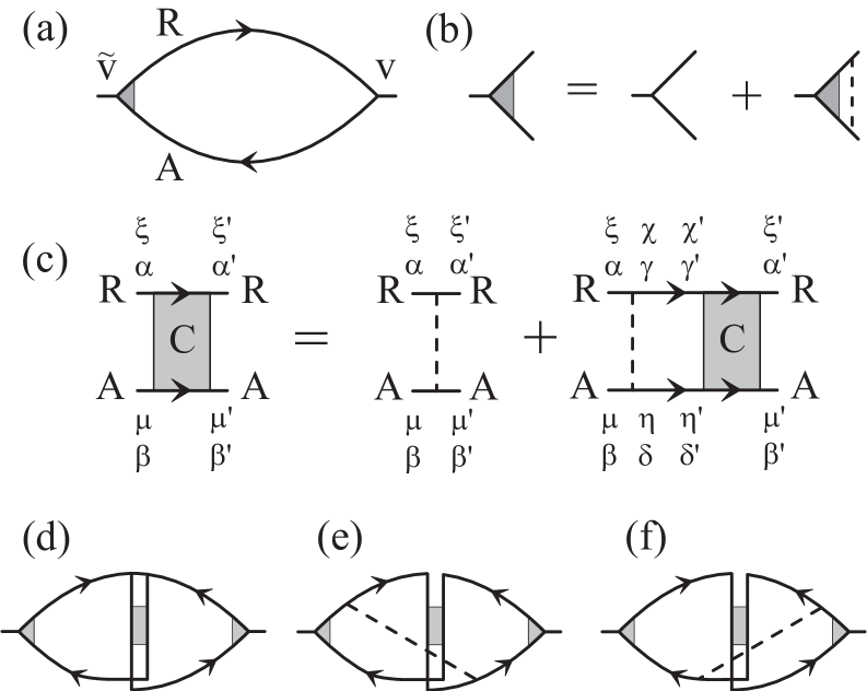
Figure 4: (a) Diagram for the Drude conductivity with (b) the vertex correction. (c) Bethe-Salpeter equation for the Cooperon propagator with valley indices $\xi\mu\xi^{\prime}\mu^{\prime}$ and AB lattice indices $\alpha\beta\alpha^{\prime}\beta^{\prime}$. (d) Bare ’Hikami box’ relating the conductivity correction to the Cooperon propagator with (e) and (f) dressed ’Hikami boxes’. Solid lines represent disorder averaged $G^{R/A}$, dashed lines represent disorder.

The Cooperon $C_{\alpha\beta,\alpha^{\prime}\beta^{\prime}}^{\xi\mu,\xi^{\prime}\mu^{\prime}}$ obeys the Bethe-Salpeter equation represented diagrammatically in figure 4(c). The shaded blocks in figure 4(c) are infinite series of ladder diagrams, while the dashed lines represent the correlator of the disorder in equation (8). We classify Cooperons in graphene as iso- and pseudospin singlets and triplets, as was mentioned above, with the help of the following relation,

$$C_{s_{1}s_{2}}^{l_{1}l_{2}}=\frac{1}{4}\sum_{\alpha,\beta,\alpha^{\prime},\beta^{\prime},}\sum_{\xi,\mu,\xi^{\prime},\mu^{\prime},}\left(\Sigma_{y}\Sigma_{s_{1}}\Lambda_{y}\Lambda_{l_{1}}\right)_{\alpha\beta}^{\xi\mu}C_{\alpha\beta,\alpha^{\prime}\beta^{\prime}}^{\xi\mu,\xi^{\prime}\mu^{\prime}}\left(\Sigma_{s_{2}}\Sigma_{y}\Lambda_{l_{2}}\Lambda_{y}\right)_{\beta^{\prime}\alpha^{\prime}}^{\mu^{\prime}\xi^{\prime}}\,.$$ (10)

Such a classification of modes is permitted by the commutation of the iso- and pseudospin operators $\vec{\Sigma}$ and $\vec{\Lambda}$ in Eqs. (6,7,10), $[\Sigma_{s},\Lambda_{l}]=0$. To select the isospin singlet ($s=0$) and triplet ($s=x,y,z$) Cooperon components (scalar and vector representation of the sublattice group SU${}_{2}^{\Sigma}\equiv\{e^{ia\vec{n}\cdot\!\vec{\Sigma}}\}$), we project the incoming and outgoing Cooperon indices onto matrices $\Sigma_{y}\Sigma_{s_{1}}$and $\Sigma_{s_{2}}\Sigma_{y}$, respectively. The pseudospin singlet ($l=0$) and triplet ($l=x,y,z$) Cooperons (scalar and vector representation of the valley group SU${}_{2}^{\Lambda}\equiv\{\mathrm{e}^{ib\vec{n}\cdot\!\vec{\Lambda}}\}$) are determined by the projection of $C_{\alpha\beta,\alpha^{\prime}\beta^{\prime}}^{\xi\mu,\xi^{\prime}\mu^{\prime}}$ onto matrices $\Lambda_{y}\Lambda_{l_{1}}$($\Lambda_{l_{2}}\Lambda_{y}$) and are accounted for by superscript indices in $C_{s_{1}s_{2}}^{l_{1}l_{2}}$.

For ’diagonal’ disorder $\mathrm{\hat{I}}u(\mathbf{r})$, the Bethe-Salpeter equation, figure 4(c) takes the form

$$C_{s_{1}s_{2}}^{l_{1}l_{2}}\left(\mathbf{q}\right) = \tau_{0}\,\delta^{l_{1}l_{2}}\delta_{s_{1}s_{2}}$$

$$+ \frac{1}{4\pi\gamma\tau_{0}\hbar}\sum_{s,l}C_{ss_{2}}^{ll_{2}}\left(\mathbf{q}\right)\int\frac{d^{2}p}{\left(2\pi\right)^{2}}\mathrm{Tr}\Big{\{}\Sigma_{s}\Sigma_{y}\Lambda_{l}\Lambda_{y}\left[\hat{G}_{\mathbf{p},\hbar\omega+\epsilon}^{R}\right]^{\mathrm{t}}\Lambda_{y}\Lambda_{l_{1}}\Sigma_{y}\Sigma_{s_{1}}\hat{G}_{\hbar\mathbf{q}-\mathbf{p},\epsilon}^{A}\Big{\}}.$$

It leads to a series of coupled equations for the Cooperon modes $C_{ss}^{ll}\equiv C_{s}^{l}$. It turns out that for potential disorder $\mathrm{\hat{I}}u(\mathbf{r})$ isospin-singlet modes $C_{0}^{l}$ are gapless in all (singlet and triplet) pseudospin channels, whereas triplet modes $C_{x}^{l}$ and $C_{y}^{l}$ have relaxation gaps $\Gamma_{x}^{l}=\Gamma_{y}^{l}=\frac{1}{2}\tau_{0}^{-1}$ and $C_{z}^{l}$ have gaps $\Gamma_{z}^{l}=\tau_{0}^{-1}$. When obtaining the diffusion equations for the Cooperons using the gradient expansion of the Bethe-Salpeter equation we take into account its matrix structure. We find that isospin-singlets $C_{0}^{l}$ are coupled to the triplets $C_{x}^{l}$ and $C_{y}^{l}$ in linear order in the small wavevector $\mathbf{q}$, so that the derivation of the diffusion operator for the isospin-singlet components would be incorrect if coupling to the gapful modes were neglected. The matrix equation for each set of four Cooperons

$$\mathbf{C}^{l}\equiv\left(\begin{array}[]{cccc}C_{00}^{l}&C_{0x}^{l}&C_{0y}^{l}&C_{0z}^{l}\\ C_{x0}^{l}&C_{xx}^{l}&C_{xy}^{l}&C_{xz}^{l}\\ C_{y0}^{l}&C_{yx}^{l}&C_{yy}^{l}&C_{yz}^{l}\\ C_{z0}^{l}&C_{zx}^{l}&C_{zy}^{l}&C_{zz}^{l}\\ \end{array}\right),$$

has the form

$$\left(\begin{array}[]{cccc}\frac{1}{2}v^{2}\tau_{0}q^{2}+\Gamma_{0}^{l}-i\omega&\frac{-i}{2}vq_{x}&\frac{-i}{2}vq_{y}&0\\ \frac{-i}{2}vq_{x}&\frac{1}{2}\tau_{0}^{-1}&0&0\\ \frac{-i}{2}vq_{y}&0&\frac{1}{2}\tau_{0}^{-1}&0\\ 0&0&0&\tau_{0}^{-1}\end{array}\right)\mathbf{C}^{l}=1.$$ (13)

After the isospin-triplet modes are eliminated, the diffusion operator for each of the four gapless/low-gap modes $C_{0}^{l}$ becomes $Dq^{2}-i\omega+\Gamma_{0}^{l}$, where $D=\frac{1}{2}v^{2}\tau_{\mathrm{tr}}=v^{2}\tau_{0}$.

Symmetry-breaking perturbations lead to relaxation gaps $\Gamma_{0}^{l}$ in the otherwise gapless pseudo-spin-triplet components of the isospin-singlet Cooperon $C_{0}^{l}$. All scattering mechanisms described in equation (8) should be included in the corresponding disorder correlator (dashed line) on the r.h.s. of the Bethe-Salpeter equation and in the scattering rate in the disorder-averaged $G^{R/A}$, as $\tau_{\mathrm{0}}^{-1}\rightarrow\tau^{-1}=\tau_{\mathrm{0}}^{-1}+\sum_{sl}\tau_{sl}^{-1}$. This opens relaxation gaps in all pseudospin-triplet modes, $C_{0}^{x},C_{0}^{y},C_{0}^{z}$, though does not generate a relaxation of the pseudospin-singlet $C_{0}^{0}$ which is protected by particle conservation.

The trigonal warping term ${\hat{h}}_{\mathrm{1w}}$ in the free electron Hamiltonian equation (2) breaks the $\mathbf{p}\rightarrow-\mathbf{p}$ symmetry of the Fermi lines within each valley kpoints . It has been noticed EggShaped that the deformation of a Fermi line of 2D electrons in GaAs/AlGaAs heterostructures in a strong in-plane magnetic field suppresses Cooperons as soon as the deformation violates $\mathbf{p}\rightarrow-\mathbf{p}$ symmetry. As ${\hat{h}}_{\mathrm{1w}}$ has a similar effect, it enhances the relaxation rate of the pseudospin-triplet intravalley components $C_{0}^{x}$ and $C_{0}^{y}$ by

$$\tau_{\mathrm{w}}^{-1}=2\tau_{0}\left(\epsilon^{2}\mu/\hbar v^{2}\right)^{2}.$$ (14)

The estimated warping-induced relaxation time is rather short for all electron densities in the samples studied in [17], $\tau_{\mathrm{w}}/\tau_{\mathrm{tr}}\sim 5-30,\tau_{\mathrm{w}}<\tau_{\varphi}$, which excludes any WAL determined by intravalley Cooperon components. However, since warping has an opposite effect on different valleys, it does not lead to relaxation of the pseudospin-singlet $C_{0}^{0}$ or the intervalley component of the pseudospin triplet, $C_{0}^{z}$.

Altogether, the relaxation of modes $C_{0}^{l}$ can be described by the following combinations of rates:

$$\Gamma_{0}^{0}=0,\;\Gamma_{0}^{z}=2\tau_{\mathrm{i}}^{-1},\;\Gamma_{0}^{x}=\Gamma_{0}^{y}=\tau_{\ast}^{-1}\equiv\tau_{\mathrm{w}}^{-1}+\tau_{\mathrm{z}}^{-1}+\tau_{\mathrm{i}}^{-1},$$ (15)

where $\tau_{\mathrm{i}}^{-1}$ is the intervalley scattering rate (here we use the $x-y$ plane isotropy of disorder, $\tau_{sx}^{-1}=\tau_{sy}^{-1}\equiv\tau_{s\bot}^{-1}$ and $\tau_{xl}^{-1}=\tau_{yl}^{-1}\equiv\tau_{\bot l}^{-1}$),

$$\tau_{\mathrm{i}}^{-1}=4\tau_{\bot\bot}^{-1}+2\tau_{z\bot}^{-1},\;\mathrm{and}\;\tau_{\mathrm{z}}^{-1}=4\tau_{\bot z}^{-1}+2\tau_{zz}^{-1}.$$ (16)

After we include dephasing due to an external magnetic field, $\mathbf{B}=\mathrm{rot}\mathbf{A}$ and inelastic decoherence, $\tau_{\varphi}^{-1}$, the equations for $C_{0}^{l}$ read

$$[D(i\mathbf{\nabla}+{\textstyle\frac{2e}{c\hbar}}\mathbf{A)}^{2}+\Gamma_{0}^{l}+\tau_{\varphi}^{-1}-i\omega]C_{0}^{l}\left(\mathbf{r},\mathbf{r^{\prime}}\right)=\delta\left(\mathbf{r}-\mathbf{r^{\prime}}\right).$$ (17)

2.5 Weak localization magnetoresistance in monolayer graphene

Due to the momentum-independent form of the current operator $\mathbf{\tilde{v}=2}v\vec{\Sigma}$, the WL correction to conductivity $\delta g$ includes two additional diagrams, figure 4(e) and (f) besides the standard diagram shown in figure 4(d). Each of the diagrams in figure 4(e) and (f) produces a contribution equal to $(-\frac{1}{4})$ of that in figure 4(d). This partial cancellation, together with a factor of four from the vertex corrections and a factor of two from spin degeneracy leads to

$$\delta g=\frac{2e^{2}D}{\pi\hbar}\!\int\!\frac{d^{2}q}{\left(2\pi\right)^{2}}\left(C_{0}^{x}+C_{0}^{y}+C_{0}^{z}-C_{0}^{0}\right).$$ (18)

Using equation (18), we find the $B=0$ temperature dependent correction, $\delta\rho/\rho=-\delta g/g$, to the graphene sheet resistance. Taking into account the double spin degeneracy of carriers we present

$$\frac{\delta\rho\left(0\right)}{\rho^{2}}=-\frac{e^{2}}{\pi h}\left[\ln(1+2\frac{\tau_{\varphi}}{\tau_{\mathrm{i}}})-2\ln\frac{\tau_{\varphi}/\tau_{\mathrm{tr}}}{1+\frac{\tau_{\varphi}}{\tau_{\ast}}}\right],$$ (19)

and evaluate magnetoresistance, $\rho(B)-\rho(0)\equiv$ $\Delta\rho(B)$,

$$\Delta\rho(B)=\frac{e^{2}\rho^{2}}{\pi h}\left[F(\frac{B}{B_{\varphi}})-F(\frac{B}{B_{\varphi}+2B_{\mathrm{i}}})\right.\left.-2F(\frac{B}{B_{\varphi}+B_{\ast}})\right],$$ (20)

$$F(z)=\ln z+\psi(\frac{1}{2}+\frac{1}{z}),\;B_{\varphi,\mathrm{i},\ast}=\frac{\hbar c}{4De}\tau_{\varphi,\mathrm{i},\ast}^{-1}\,.$$

Here, $\psi$ is the digamma function and the decoherence (taken into account by the rate $\tau_{\varphi}^{-1}$) determines the curvature of the magnetoresistance at $B<B_{\varphi}\equiv\hbar c/4De\tau_{\varphi}$.

The last term in equation (18), $C_{0}^{0}$ is the only true gapless Cooperon mode which determines the dominance of the WL sign in the quantum correction to the conductivity in graphene with a long phase coherence time, $\tau_{\varphi}>\tau_{\mathrm{i}}$. The two curves sketched in figure 1 illustrate the corresponding MR in two limits: $B_{\ast}\ll B_{\mathrm{i}}$ ($\tau_{\ast}\gg\tau_{\mathrm{i}}$) and $B_{\ast}\gg B_{\mathrm{i}}$ ($\tau_{\ast}\ll\tau_{\mathrm{i}}$). In both cases, the low-field MR ($B\ll B_{\mathrm{i}}$) is negative. If $B_{\ast}\ll B_{\mathrm{i}}$, the MR changes sign: $\Delta\rho(B)<0$ at $B<B_{\mathrm{i}}\equiv\hbar c/4De\tau_{\mathrm{i}}$ and $\Delta\rho(B)>0$ at higher fields. For $B_{\ast}\gg B_{\mathrm{i}}$, the MR is distinctly of a WL type, with almost no sign of WAL. Such behavior is expected in graphene tightly coupled to the insulating substrate (which generates atomically sharp scatterers). In a sheet loosely attached to a substrate (or suspended), the intervalley scattering time may be longer than the decoherence time, $\tau_{\mathrm{i}}>\tau_{\varphi}>\tau_{\mathrm{w}}$ ($B_{\mathrm{i}}<B_{\varphi}<B_{\mathrm{\ast}}$). Hence $C_{0}^{z}$ is effectively gapless, whereas trigonal warping suppresses the modes $C_{0}^{x}$ and $C_{0}^{y}$. In this case the contribution from $C_{0}^{z}$ cancels $C_{0}^{0}$, and the MR would display neither WL nor WAL behavior: $\Delta\rho(B)=0$.

3 Weak localisation magnetoresistance in disordered bilayer graphene

3.1 Low energy Hamiltonian of bilayer graphene

Bilayer graphene consists of two coupled monolayers. Its unit cell contains four inequivalent sites, $A,B,\tilde{A}$ and $\tilde{B}$ ($A,B$ and $\tilde{A},\tilde{B}$ lie in the bottom and top layer, respectively) arranged according to Bernal stacking dressel02 ; McCann : sites $B$ of the honeycomb lattice in the bottom layer lie exactly below $\tilde{A}$ of the top layer, figure 5. The Brillouin zone of the bilayer, similarly to the one in monolayer, has two inequivalent degeneracy points $\mathbf{K}_{+}$ and $\mathbf{K}_{-}$ which determine two valleys centered around $\epsilon=0$ in the electron spectrum kpoints . Near the center of each valley the electron spectrum consists of four branches. Two branches describing states on sublattices $\tilde{A}$ and $B$ are split from energy $\epsilon=0$ by about $\pm\gamma_{1}$, the interlayer coupling, whereas two low-energy branches are formed by states based upon sublattices $A$ and $\tilde{B}$. The latter can be described McCann using the Hamiltonian, which acts in the space of four-component wave functions $\Phi=[\phi_{\mathbf{K}_{+},A},\phi_{\mathbf{K}_{+},\tilde{B}},\phi_{\mathbf{K}_{-},\tilde{B}},\phi_{\mathbf{K}_{-},A}]$, where $\phi_{\xi,\alpha}$ is an electron amplitude on the sublattice $\alpha=A,\tilde{B}$ and in the valley $\xi=\mathbf{K_{+}},\mathbf{K_{-}}$.

$$\!\!\!\!\!\!\!\!\!\!{\hat{H}}_{2L}=-\frac{1}{2m}\left[\left({p}_{x}^{2}-{p}_{y}^{2}\right)\sigma_{x}+2{p}_{x}{p}_{y}\sigma_{y}\right]+{\hat{h}}_{\mathrm{2w}}+\hat{V}_{disorder},$$ (21)

$${\hat{h}}_{\mathrm{2w}}=v_{3}\Pi_{z}\left(p_{x}\sigma_{x}-p_{y}\sigma_{y}\right).$$

Here, $\sigma_{x,y,z}$ and $\Pi_{x,y,z}$ are Pauli matrices acting in sublattice and valley space, respectively.

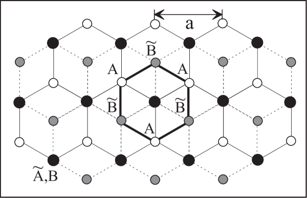
Figure 5: Schematic of the bilayer lattice (bonds in the bottom layer $A,B$ are indicated by solid lines and in the top layer $\tilde{A},\tilde{B}$ by dashed lines) containing four sites in the unit cell: $A$ (white circles), $\tilde{B}$ (grey), $\tilde{A}B$ dimer (black).

The first term in equation (21) is the leading contribution in the nearest neighbors approximation of the tight binding model McCann . This approximation takes into account both intralayer hopping $A\leftrightarrow B$ and $\tilde{A}\leftrightarrow\tilde{B}$ (that leads to the Dirac-type dispersion $\epsilon=\pm pv$ near the Fermi point $\mathbf{K_{\pm}}$ in a monolayer) and the interlayer $\tilde{A}\leftrightarrow B$ hopping. This term yields the parabolic spectrum $\epsilon=\pm p^{2}/2m$ with $m=\gamma_{1}/2v^{2}$ which dominates in the intermediate energy range $\frac{1}{4}\gamma_{1}(v_{3}/v)^{2}<\varepsilon_{F}<\frac{1}{4}\gamma_{1}$. In this regime we can truncate the expansion of $\hat{H}(\mathbf{p})$ in powers of the momentum $\mathbf{p}$ neglecting terms of the order higher than quadratic. Electron waves characteristic for the first, quadratic, term of ${\hat{H}}_{2L}$ have the form

$$\Phi_{\mathbf{K},\pm\mathbf{p}}=\pm\frac{e^{\pm i\mathbf{px}/\hbar}}{\sqrt{2}}\left(e^{-i\varphi}|\uparrow\rangle_{\mathbf{K},\pm\mathbf{p}}-e^{i\varphi}|\downarrow\rangle_{\mathbf{K},\pm\mathbf{p}}\right),$$ (22)

where ${|\uparrow\rangle_{\mathbf{K}_{+},\pm\mathbf{p}}}=[1,0,0,0]$, ${|\downarrow\rangle_{\mathbf{K}_{+},\pm\mathbf{p}}}=[0,1,0,0]$ and ${|\uparrow\rangle_{\mathbf{K}_{-},\pm\mathbf{p}}}=[0,0,1,0]$, ${|\uparrow\rangle_{\mathbf{K}_{-},\pm\mathbf{p}}}=[0,0,0,1]$. These are eigenstates of an operator $\mathbf{\sigma n}_{2}$ with $\mathbf{\sigma n}_{2}=-1$ for electrons in the conduction band and $\mathbf{\sigma n}_{2}=1$ for electrons in the valence band, where $\mathbf{n}_{2}(\mathbf{p})=(\textrm{cos}(2\varphi),\textrm{sin}(2\varphi))$ for $\mathbf{p}=(p\textrm{cos}\varphi,p\textrm{sin}\varphi)$, which means that they are chiral, but with the degree of chirality different from the one found in monolayer (see Sec. 2.1). Such electron waves are characterized by the Berry phase $2\pi$, and the dependence $w(\theta)\sim\cos^{2}\theta$ of the scattering probability off a short-range potential on the scattering angle $\theta=\widehat{\mathbf{pp}}\mathbf{{}^{\prime}}$ is such that transport and scattering times in the bilayer coincide, although $w(\theta)$ is anisotropic [see figure 3(c)], and the Drude conductivity of a bilayer is $g=4e^{2}n\tau_{0}/m$ (in contrast to monolayer graphene, see Sec. 2.1).

The second term in equation (21), ${\hat{h}}_{2\mathrm{w}}$, originates from a weak direct $A\leftrightarrow\tilde{B}$ interlayer coupling. It leads to a Lifshitz transition in the shape of the Fermi line of the 2D electron gas which takes place when $\epsilon_{\mathrm{F}}\sim\epsilon_{\mathrm{L}}\equiv\frac{1}{4}\gamma_{1}(v_{3}/v)^{2}$. In a bilayer with $\epsilon_{\mathrm{F}}<\epsilon_{\mathrm{L}}$, the interplay between the two terms in ${\hat{H}}_{2L}$ determines the Fermi line in the form of four pockets McCann in each valley. In a bilayer with $\epsilon_{\mathrm{F}}>\epsilon_{\mathrm{L}}$, ${\hat{h}}_{\mathrm{2w}}$ can be treated as a perturbation leading to a trigonal deformation of a single-connected Fermi line, thus manifesting the asymmetry of the electron dispersion inside each valley: $\epsilon(\mathbf{K}_{\pm},\mathbf{p})\neq\epsilon(\mathbf{K}_{\pm},-\mathbf{p})$. This asymmetry leads to the dephasing effect of electron trajectories similar to the one discussed in the case of monolayer, and is characterized by the scattering rate $\tau_{\mathrm{w}}^{-1}$ equation (5).

The term $\hat{V}_{disorder}$ in the equation (21) describes time-reversal-symmetric disorder. It is parameterized using $t\rightarrow-t$ symmetric $4\times 4$ matrices acting in the sublattice/valley space, which are listed in Table 3.

$$\hat{V}_{disorder}=\sum_{s,l=0,x,y}\Pi_{l}\sigma_{s}u_{sl}(\mathbf{r})+\Pi_{z}\sigma_{z}u_{zz}(\mathbf{r}).$$ (23)

The sum in equation (23) contains valley and isospin conserving disorder potential $\hat{I}u(\mathbf{r})$, with $\langle u(\mathbf{r})u(\mathbf{r^{\prime}})\rangle=u^{2}\delta(\mathbf{r}-\mathbf{r^{\prime}})$ and $\tau^{-1}_{0}=\pi\gamma u^{2}/\hbar,\gamma={\textstyle\frac{m}{2\pi}}$, which originates from charged impurities in the $\textrm{SiO}_{2}$ substrate and is assumed to be the dominant mechanism of scattering in the system. All other types of disorder which breaks valley and sublattice symmetries are assumed to be uncorrelated, $\langle u_{s\,l}(\mathbf{r})u_{s^{\prime}\,l^{\prime}}(\mathbf{r^{\prime}})\rangle=u_{s\,l}^{2}\delta_{ss^{\prime}}\delta_{ll^{\prime}}\delta(\mathbf{r}-\mathbf{r^{\prime}})$. We characterize them using scattering rates $\tau^{-1}_{s\,l}=\pi\gamma u^{2}_{s\,l}/\hbar$. Furthermore, the scattering is assumed to be isotropic in the $x-y$ plane, so that $u^{2}_{xl}=u^{2}_{yl}\equiv u^{2}_{\perp l},u^{2}_{s\,x}=u^{2}_{sy}\equiv u^{2}_{s\perp}$.

Table 3: Transformations of matrices of the form ${\Pi}_{l}{\sigma}_{s},s,l=0,x,y,z$, under crystalline symmetry group generators and time reversal operation. In bilayer graphene rotations and reflection symmetry operators are multiplied by the operation of reflection with respect to the $z=0$ plane, which is equidistant with respect to two honeycomb lattice layers. Therefore symmetry group generators are ${\textstyle\frac{\pi}{3}}$-rotation, $C_{6}R_{z}$, mirror reflection with respect to $Ox$ axis, $R_{x}R_{z}$, and translation along $Ox$ by lattice constant, $\mathbf{a}$. Operation $T$ stands for the time reversal, $t\rightarrow-t$. Here matrices are grouped into bases forming irreducible representations of the symmetry group which can be $1,2$ and 4 dimensional. The transformation matrixes $U_{ji}$, $g\phi_{i}=\sum_{j}U_{ji}(g)\phi_{j}$ ($g$ stands for a symmetry operation), are given explicitly for each of such bases $\phi_{i}$.

$\Pi_{l}\sigma_{s}$	$T$	$C_{6}R_{z}$	$R_{x}R_{z}$	$\mathbf{a}$
$\hat{I}$	$+1$	$+1$	$+1$	$+1$
$\Pi_{0}\sigma_{z}$	$-1$	$+1$	$-1$	$+1$
$\Pi_{z}\sigma_{0}$	$-1$	$-1$	$+1$	$+1$
$\Pi_{z}\sigma_{z}$	$+1$	$-1$	$-1$	$+1$
$\left[\begin{array}[]{cc}\Pi_{0}\sigma_{x}&\\ \Pi_{0}\sigma_{y}&\\ \end{array}\right]$	$+1$	$\left(\begin{array}[]{cc}-\frac{1}{2}&\frac{\sqrt{3}}{2}\\ -\frac{\sqrt{3}}{2}&-\frac{1}{2}\\ \end{array}\right)$	$\left(\begin{array}[]{cc}1&0\\ 0&-1\\ \end{array}\right)$	$\left(\begin{array}[]{cc}1&0\\ 0&1\\ \end{array}\right)$
$\left[\begin{array}[]{cc}\Pi_{z}\sigma_{x}\\ \Pi_{z}\sigma_{y}\\ \end{array}\right]$	$-1$	$\left(\begin{array}[]{cc}\frac{1}{2}&-\frac{\sqrt{3}}{2}\\ \frac{\sqrt{3}}{2}&\frac{1}{2}\\ \end{array}\right)$	$\left(\begin{array}[]{cc}1&0\\ 0&-1\\ \end{array}\right)$	$\left(\begin{array}[]{cc}1&0\\ 0&1\\ \end{array}\right)$
$\left[\begin{array}[]{cc}\Pi_{x}\sigma_{0}\\ \Pi_{y}\sigma_{0}\\ \end{array}\right]$	$+1$	$\left(\begin{array}[]{cc}1&0\\ 0&-1\\ \end{array}\right)$	$\left(\begin{array}[]{cc}1&0\\ 0&1\\ \end{array}\right)$	$\left(\begin{array}[]{cc}-\frac{1}{2}&-\frac{\sqrt{3}}{2}\\ \frac{\sqrt{3}}{2}&-\frac{1}{2}\\ \end{array}\right)$
$\left[\begin{array}[]{cc}\Pi_{x}\sigma_{z}\\ \Pi_{y}\sigma_{z}\\ \end{array}\right]$	$-1$	$\left(\begin{array}[]{cc}1&0\\ 0&-1\\ \end{array}\right)$	$\left(\begin{array}[]{cc}1&0\\ 0&1\\ \end{array}\right)$	$\left(\begin{array}[]{cc}-\frac{1}{2}&-\frac{\sqrt{3}}{2}\\ \frac{\sqrt{3}}{2}&-\frac{1}{2}\\ \end{array}\right)$
$\left[\begin{array}[]{cccc}\Pi_{x}\sigma_{x}\\ \Pi_{x}\sigma_{y}\\ \Pi_{y}\sigma_{x}\\ \Pi_{y}\sigma_{y}\\ \end{array}\right]$	$+1$	$\left(\begin{array}[]{cccc}-\frac{1}{2}&\frac{\sqrt{3}}{2}&0&0\\ -\frac{\sqrt{3}}{2}&-\frac{1}{2}&0&0\\ 0&0&\frac{1}{2}&-\frac{\sqrt{3}}{2}\\ 0&0&\frac{\sqrt{3}}{2}&\frac{1}{2}\\ \end{array}\right)$	$\left(\begin{array}[]{cccc}1&0&0&0\\ 0&-1&0&0\\ 0&0&1&0\\ 0&0&0&-1\\ \end{array}\right)$	$\left(\begin{array}[]{cccc}-\frac{1}{2}&0&-\frac{\sqrt{3}}{2}&0\\ 0&-\frac{1}{2}&0&-\frac{\sqrt{3}}{2}\\ \frac{\sqrt{3}}{2}&0&-\frac{1}{2}&0\\ 0&\frac{\sqrt{3}}{2}&0&-\frac{1}{2}\\ \end{array}\right)$

3.2 Interference of electronic waves in bilayer graphene

To analyze the WL effect we introduce Cooperon matrix $C_{\alpha\beta\alpha^{\prime}\beta^{\prime}}^{\xi\mu\xi^{\prime}\mu^{\prime}}$ where subscripts describe the sublattice state of incoming $\alpha\beta$ and outgoing $\alpha^{\prime}\beta^{\prime}$ pairs of electrons and superscripts describe the valley state of incoming $\xi\mu$ and outgoing $\xi^{\prime}\mu^{\prime}$ pairs. Note that in contrast to monolayer we do not rewrite the bilayer Hamiltonian in terms of $\Sigma$ and $\Lambda$ matrices. We parametrize Cooperons as $C_{S_{1}S_{2}}^{M_{1}M_{2}}$ by $M_{1},M_{2}$ ”valley” and $S_{1},S_{2}$ ”sublattice” singlet and triplet states in a similar way to monolayer isospin and pseudospin states. The sublattice composition of Cooperons is determined by the correlator of plane waves propagating ballistically in opposite directions,

$$\Phi_{\mathbf{K},\mathbf{p}}\Phi_{\mathbf{K}^{\prime},-\mathbf{p}}\!\sim\!{|\uparrow\rangle}_{\mathbf{K},\mathbf{p}}|\downarrow\rangle_{\mathbf{K}^{\prime},-\mathbf{p}}\!+\!|\downarrow\rangle_{\mathbf{K},\mathbf{p}}|\uparrow\rangle_{\mathbf{K}^{\prime},-\mathbf{p}}\!-e^{2i\varphi}|\uparrow\rangle_{\mathbf{K},\mathbf{p}}|\uparrow\rangle_{\mathbf{K}^{\prime},-\mathbf{p}}\!-e^{-2i\varphi}|\downarrow\rangle_{\mathbf{K},\mathbf{p}}|\downarrow\rangle_{\mathbf{K}^{\prime},-\mathbf{p}}.$$

It is seen from the above expression that after averaging over the momentum direction the terms corresponding to $C_{x,y}^{M}\propto({|\uparrow\rangle_{\mathbf{K},\mathbf{p}}}{|\uparrow\rangle_{\mathbf{K^{\prime}},-\mathbf{p}}}\pm{|\downarrow\rangle_{\mathbf{K},\mathbf{p}}}{|\downarrow\rangle_{\mathbf{K^{\prime}},-\mathbf{p}}})$ disappear, since $\mathbf{p}=(p\cos\varphi,p\sin\varphi)$ so that $\langle e^{\pm 2i\varphi}\rangle_{\varphi}=0$, whereas terms correponding to the sublattice symmetric Cooperons, $C_{z}^{M}\propto({|\uparrow\rangle_{\mathbf{K},\mathbf{p}}}{|\downarrow\rangle_{\mathbf{K^{\prime}},-\mathbf{p}}}+{|\downarrow\rangle_{\mathbf{K},\mathbf{p}}}{|\uparrow\rangle_{\mathbf{K^{\prime}},-\mathbf{p}}})$ remain non-zero.

The dephasing effect of trigonal warping in bilayer is similar to monolayer, although it is caused by a different mechanism, its magnitude is estimated by equation (5). Dephasing due to warping suppresses the intravalley Cooperons $C_{z}^{x,y}$ leading to the absence of WL magnetoresistance in the case of weak intervalley scattering, $\tau_{\mathrm{i}}\gg\tau_{\varphi}$. In the case of strong intervalley scattering, $\tau_{\mathrm{i}}\ll\tau_{\varphi}$, WL is partially restored, thus, we predict the WL behavior of bilayer graphene with strong trigonal warping of Fermi line in each valley to be described by equation (1).

3.3 Diagrammatic calculation of the weak localization correction in bilayer graphene

We derive the disorder averaged Green function for the bilayer Hamiltonian equation (21):

$$G^{R/A}\left(\mathbf{p},\epsilon\right)=\frac{\epsilon_{R/A}-\epsilon_{p}\,\mathbf{\sigma n_{2}}(\mathbf{p})}{\epsilon_{R/A}^{2}-\epsilon_{p}^{2}},$$ (24)

where $\epsilon_{R/A}=\epsilon\pm{\textstyle\frac{1}{2}}i\hbar\tau^{-1}$ and $\tau^{-1}=\tau_{0}^{-1}+\tau_{\mathrm{i}}^{-1}+\tau_{\mathrm{z}}^{-1}\approx\tau_{0}^{-1}$. Here we introduced the following notations for the scattering rates $\tau_{sl}^{-1}=\pi\gamma u_{sl}^{2}/\hbar$, where $\tau_{sx}^{-1}=\tau_{sy}^{-1}\equiv\tau_{s\bot}^{-1}$ and $\tau_{xl}^{-1}=\tau_{yl}^{-1}\equiv\tau_{\bot l}^{-1}$ can be combined into the intervalley scattering rate $\tau_{\mathrm{i}}^{-1}=4\tau_{\bot\bot}^{-1}+2\tau_{z\bot}^{-1}$ and the intravalley rate $\tau_{\mathrm{z}}^{-1}=\tau_{zz}^{-1}$ both of which lead to an additional suppression of intravalley modes. Intervalley scattering also leads to the relaxation of $C_{z}^{0}$ although it does not affect the valley-symmetric mode $C_{z}^{z}$. Together, all the scattering mechanisms limit the transport time $\tau^{-1}=\tau_{0}^{-1}+\sum_{sl}\tau_{sl}^{-1}$.

Due to quadratic spectrum of quasiparticles in bilayer graphene the velocity operator, $\hat{v}_{x}=-(p_{x}\sigma_{x}+p_{y}\sigma_{y})/m$, $\hat{v}_{y}=(p_{y}\sigma_{x}-p_{x}\sigma_{y})/m$, is momentum dependent, and thus the current vertices in the conductivity diagram figure 4(c) are not renormalized by impurity scattering accounted for by the diagram series figure 4(b). As a result, the Drude conductivity is described by $g=4e^{2}\nu D$, where $D={\textstyle\frac{1}{2}}v^{2}_{F}\tau_{0}$ and $\tau_{tr}=\tau_{0}$.

We parametrize the Cooperons utilizing the expression,

$$C^{M_{1}M_{2}}_{S_{1}S_{2}} = \frac{1}{4}\sum_{\alpha,\beta,\alpha^{\prime},\beta^{\prime}}\sum_{\xi,\mu,\xi^{\prime},\mu^{\prime}}\left(\sigma_{y}\sigma_{S_{1}}\right)_{\alpha\beta}\left(\Pi_{y}\Pi_{\kappa_{1}}\right)^{\xi\mu}C^{\;\xi\mu,\xi^{\prime}\mu}_{\alpha\beta,\alpha^{\prime}\beta^{\prime}}\left(\sigma_{S_{2}}\sigma_{y}\right)_{\beta^{\prime}\alpha^{\prime}}\left(\Pi_{\kappa_{2}}\Pi_{y}\right)^{\mu^{\prime}\xi^{\prime}}.$$

The Bethe-Salpeter equation for Cooperons in bilayer reads,

$$C_{S_{1}S_{2}}^{M_{1}M_{2}}\left(\mathbf{q}\right) = \tau_{0}\,\delta_{M_{1},M_{2}}\delta_{S_{1},S_{2}}$$ (25)

$$\!\!\!\!\!\!\!\!\!\!\!\!\!\!\!\!\!\!\!\!\!\!\!\!\!\!\!\!\!\!\!\!\!\!\!\!\!\!\!\!\!\!\!\!\!\!\!\!\!\!\!\!\!+ \!\!\!\!\!\!\!\!\!\!\!\!\!\!\!\!\!\!\!\!\!\!\!\!\!\!\!\frac{1}{4\pi\gamma\tau_{0}\hbar}\sum_{S,M}C_{SS_{2}}^{MM_{2}}\left(\mathbf{q}\right)\int\frac{d^{2}p}{\left(2\pi\right)^{2}}\mathrm{Tr}\Big{\{}\Pi_{M}\sigma_{S}\Pi_{y}\sigma_{y}\left[G_{\mathbf{p},\hbar\omega+\epsilon}^{R}\right]^{\mathrm{t}}\Pi_{y}\sigma_{y}\Pi_{M_{1}}\sigma_{S_{1}}G_{\hbar\mathbf{q}-\mathbf{p},\epsilon}^{A}\Big{\}}.$$

We find that $C_{SS^{\prime}}^{MM^{\prime}}=\delta^{MM^{\prime}}\delta_{SS^{\prime}}C_{S}^{M}$ and that sublattice-singlet $C_{0}^{M}$ has a relaxation gap $\Gamma_{0}^{M}=\tau_{0}^{-1}$, sublattice-triplets $C_{x}^{M}$, $C_{y}^{M}$ have gaps $\Gamma_{x}^{M}=\Gamma_{y}^{M}=\frac{1}{2}\tau_{0}^{-1}$, whereas symmetric sublattice-triplet Cooperon $C_{z}^{M}$ is gapless. Due to warping of the Fermi line induced by ${\hat{h}_{2w}}$ in the free-electron Hamiltonian (21), the intravalley Cooperons $C_{z}^{x}$, $C_{z}^{y}$ are suppressed, even in a bilayer with purely potential disorder. Warping opens a gap, $\tau_{\mathrm{w}}^{-1}$ in the relaxation spectrum of these ‘valley-triplet’ Cooperon components:

$$\tau_{\mathrm{w}}^{-1}=\left\{\begin{array}[]{cc}{\textstyle\frac{1}{2\hbar^{2}}}\tau\langle\mathrm{Tr}{\hat{h}}_{\mathrm{w}}^{2}(\mathbf{p})\rangle_{\varphi}=\pi n_{L}l^{2}\tau^{-1},&\pi n_{L}l^{2}<1\\ \!\!\!\!\!\!\!\!\!\!\!\!\!\!\!\!\!\!\!\!\!\!\!\!\!\!\!\!\!\!\!\!\!\!\!\!\!\!\!\!\!\!\!\!\!\!\!\!\!\!\!\!\!\!\!\!\!\tau^{-1},&\pi n_{L}l^{2}>1\\ \end{array}\right.,$$ (26)

where $n_{L}$ is the density of electrons at which Lifshitz transition occurs, $l$ and $\tau$ are mean free path and transport time in the system respectively. We estimate that for the recently studied bilayers QHEbi with $n_{e}=2.5\times 10^{12}\textrm{cm}^{-2}$, $\tau_{\mathrm{w}}\sim\tau$ and the mean free path $l\sim 0.1\mu\textrm{m}$. A similar situation occurs in bilayer structures studied by R. Gorbachev et al. exeter . Also, a short-range symmetry-breaking disorder $u_{ij}$ generating intervalley scattering leads to the relaxation of $C_{z}^{0}$, although it does not affect the valley-symmetric mode $C_{z}^{z}$. Thus we find that the low-gap modes $C_{z}^{M}$ obey the diffusion equation,

$$\!\!\!\!\!\!\!\!\left[\Gamma+\tau_{\varphi}^{-1}+D(i\mathbf{\nabla}+{\textstyle\frac{2e}{c\hbar}}\mathbf{A)}^{2}-i\omega\right]C\left(\mathbf{r},\mathbf{r^{\prime}}\right)=\delta\left(\mathbf{r}-\mathbf{r^{\prime}}\right),$$

$$\!\!\!\!\!\!\!\!\Gamma_{z}^{z}=0,\;\Gamma_{z}^{0}=2\tau_{\mathrm{i}}^{-1},\;$$ (27)

$$\!\!\!\!\!\!\!\!\Gamma_{z}^{x(y)}=\tau_{\ast}^{-1}\equiv\tau_{\mathrm{w}}^{-1}+2\tau_{\mathrm{z}}^{-1}+\tau_{\mathrm{i}}^{-1},$$

where we included dephasing due to an external magnetic field, $\mathbf{B}=\mathrm{rot}\mathbf{A}$, temperature-dependent inelastic decoherence, $\tau_{\varphi}^{-1}(T)$, and all of the above mentioned relaxation mechanisms.

3.4 Weak localization magnetoresistance in bilayer graphene

The interference correction to the conductivity in a bilayer can be expressed in terms of $C\left(\mathbf{r},\mathbf{r}\right)$, the solutions of the above Cooperon equations taken at coinciding coordinates:

$$\delta g=\frac{2e^{2}D}{\pi\hbar}\left[-C_{z}^{z}+C_{z}^{0}-C_{z}^{x}-C_{z}^{y}\right].$$ (28)

For completeness, in equation (28) we have retained the intravalley Cooperons $C_{z}^{x,y}$, though they are strongly suppressed by trigonal warping. Following their suppression, the WL correction is determined by the intervalley modes $C_{z}^{0}$ and $C_{z}^{z}$ but, in the absence of intervalley scattering, the contributions of $C_{z}^{0}$ and $C_{z}^{z}$ are equal in magnitude, so that they cancel. Intervalley scattering due to atomically sharp scatterers breaks this exact cancellation and partially restores the WL effect. Equations (28,3.3) yield the zero field WL correction to the resistivity and the WL MR,

$$\frac{\delta\rho\left(0\right)}{\rho} = \frac{e^{2}\rho}{\pi h}\ln\left(1+2\frac{\tau_{\varphi}}{\tau_{\mathrm{i}}}\right)+\delta_{0},$$ (29)

$$\frac{\Delta\rho(B)}{\rho} = -\frac{e^{2}\rho}{\pi h}\left[F(\frac{B}{B_{\varphi}})-F(\frac{B}{B_{\varphi}+2B_{\mathrm{i}}})\right]+\delta(B),$$

where $B_{\varphi,\mathrm{i}}=\hbar c/(4De\tau_{\varphi,\mathrm{i}})$. Equation (29) gives a complete description of the crossover between two extreme regimes mentioned at the beginning socomment . It also includes small contributions of the suppressed intravalley Cooperons, $\delta_{0}=[2e^{2}\rho/(\pi h)]\ln(\tau_{\varphi}\tau_{\ast}/[\tau(\tau_{\ast}+\tau_{\varphi})])$ and $\delta(B)=-[2e^{2}\rho/(\pi h)]F[B/(B_{\varphi}+B_{\ast})]$, where $\tau_{\ast}^{-1}=\tau_{\mathrm{w}}^{-1}+2\tau_{\mathrm{z}}^{-1}+\tau_{\mathrm{i}}^{-1}$ and $B_{\ast}=\hbar c/(4De\tau_{\ast})$. This permits us to account for a possible difference between the warping time $\tau_{\mathrm{w}}$ and the transport time $\tau$. According to equation (29) WL MR in bilayer graphene sheet disappears as soon as $\tau_{\mathrm{i}}$ exceeds $\tau_{\varphi}$, whereas in structures with $\tau_{\varphi}>\tau_{\mathrm{i}}$, the result equation (29) predicts the WL behaviour, as observed in exeter . Such WL MR is saturated at a magnetic field determined by the intervalley scattering time, instead of the transport time as in usual conductors, which provides the possibility to measure $\tau_{\mathrm{i}}$ directly.

4 Conclusions and the effect of edges in a disordered nanoribbon

We have shown that $\mathbf{p}\rightarrow-\mathbf{p}$ asymmetry of the electron dispersion in each valley of graphene leads to unusual (for conventional disordered conductors) behavior of interference effects in electronic transport. Without intervalley scattering, trigonal warping of the electron dispersion near the center of each valley destroys the manifestation of chirality in the localization properties, resulting in a suppression of weak anti-localization in monolayer graphene and of weak localization in a bilayer. Intervalley scattering tends to restore weak localization, and this behavior is universal for monolayer and bilayer graphene, despite the fact that electrons in these two materials have different chiralities and can be attributed different Berry phases: $\pi$ in monolayers, $2\pi$ in bilayers haldane88 ; McCann . This suggests that a suppressed weak localization magnetoresistance and its sensitivity to intervalley scattering are specific to all ultrathin graphitic films independently of their morphology berger and are determined by the lower (trigonal) symmetry group of the wavevector $\mathbf{K}$ in the corner of the hexagonal Brillouin zone of a honeycomb lattice crystal.

The influence of intervalley scattering on the WL behavior determines a typically negative (WL) MR in graphene nanoribbons. Indeed, in a narrow ribbon of graphene, monolayer or bilayer, with the transverse diffusion time $L_{\bot}^{2}/D\ll\tau_{\mathrm{i}},\tau_{\ast},\tau_{\varphi}$, the sample edges determine strong intervalley scattering rate edge . Thus, when solving Cooperon equations in a wire, we estimate $\Gamma_{0}^{l}\sim\pi^{2}D/L_{\bot}^{2}$ for the pseudospin triplet, whereas the singlet $C_{0}^{0}$ remains gapless. This yields negative MR persistent over the field range $B<2\pi B_{\bot}$, where $B_{\bot}\equiv\hbar c/eL_{\bot}^{2}$:

$$\frac{\Delta\rho_{\mathrm{wire}}\left(B\right)}{\rho^{2}}=\frac{2e^{2}L_{\varphi}}{h}\,\left[\frac{1}{\sqrt{1+\frac{1}{3}B^{2}/B_{\varphi}B_{\bot}}}-1\right].$$ (30)

The results of Eqs. (19,20,28,29), and (30) give a complete description of the WL effect in graphene and describe how the WL magnetoresistance reflects the degree of valley symmetry breaking in it.

This project has been funded by Lancaster-EPSRC Portfolio Partnership grant EP/C511743 and was completed during the MPI PKS Seminar ”Dynamics and Relaxation in Complex Quantum and Classical Systems and Nanostructures.”

References

- (1) D. DiVincenzo and E. Mele, Phys. Rev. B 29, (1984) 1685.
- (2) G.W. Semenoff, Phys. Rev. Lett. 53, (1984) 2449.
- (3) F.D.M. Haldane, Phys. Rev. Lett. 61, (1988) 2015; Y. Zheng and T. Ando, Phys. Rev. B 65, (2002) 245420; V. P. Gusynin and S. G. Sharapov, Phys. Rev. Lett. 95, (2005) 146801; N.M.R. Peres, F. Guinea, and A.H. Castro Neto, Physical Review B 73, (2006) 125411; A.H. Castro Neto, F. Guinea, and N.M.R. Peres, Phys. Rev. B 73, (2006) 205408.
- (4) T. Ando, T. Nakanishi, R. Saito, J. Phys. Soc. Japan 67, (1998) 2857.
- (5) E. McCann and V.I. Fal’ko, Phys. Rev. Lett. 96, (2006) 086805; J. Nilsson et al., Phys. Rev. B 73, (2006) 214418; F. Guinea, A.H. Castro Neto, and N.M.R. Peres, ibid. 73, (2006) 245426; M. Koshino and T. Ando, ibid. 73, (2006) 245403; B. Partoens and F.M. Peeters, ibid. 74, (2006) 075404.
- (6) K.S. Novoselov et al., Science 306, (2004) 666.
- (7) K.S. Novoselov et al., Nature 438, (2005) 197.
- (8) Y. Zhang et al., Phys. Rev. Lett. 94, (2005) 176803; Nature 438, (2005) 201.
- (9) K.S. Novoselov et al., Nature Physics 2, (2006) 177.
- (10) H. Suzuura and T. Ando, Phys. Rev. Lett. 89, (2002) 266603.
- (11) B.L. Altshuler, D. Khmel’nitzkii, A.I. Larkin, and P.A. Lee, Phys. Rev. B 22, (1980) 5142.
- (12) S. Hikami, A.I. Larkin, and Y. Nagaoka, Prog. Theor. Phys. 63, (1980) 707; B.L. Al’tshuler et al., Sov. Phys. JETP 54, (1981) 411 [Zh. Eksp. Teor. Fiz. 81, (1981) 768].
- (13) D.V. Khveshchenko, Phys. Rev. Lett. 97, (2006) 036802.
- (14) A.F. Morpurgo and F. Guinea, Phys. Rev. Lett. 97, (2006) 196804.
- (15) E. McCann, K. Kechedzhi, V.I. Fal’ko, H. Suzuura, T. Ando, and B.L. Altshuler, Phys. Rev. Lett. 97, (2006) 146805.
- (16) K. Kechedzhi et al., cond-mat/0701690.
- (17) S.V. Morozov et al., Phys. Rev. Lett. 97, 016801 (2006).
- (18) R.V. Gorbachev et al., cond-mat/0701686.
- (19) X. Wu et al., cond-mat/0611339.
- (20) V. Cheianov and V.I. Fal’ko, Phys. Rev. B 74, (2006) 041403.
- (21) P.D. Dresselhaus et al., Phys. Rev. Lett. 68, (1992) 106; G.L. Chen et al., Phys. Rev. B 47, (1993) 4084; J.B. Miller et al., Phys. Rev. Lett. 90, (2003) 076807; A.L. Shelankov, Solid State Commun. 53, (1985) 465.
- (22) H. Fukuyama, J. Phys. Soc. Japan 49, (1980) 649; Prog. Theor. Phys. Suppl. 69, (1980) 220.
- (23) D.J. Bishop, D.C. Tsui, and R.C. Dynes, Phys. Rev. Lett. 44, (1980) 1153; Y. Kawaguchi and S. Kawaji, J. Phys. Soc. Jp. 48, (1980) 699; R.G. Wheeler, Phys. Rev. B 24, (1981) 4645; R.A. Davies, M.J. Uren, and M. Pepper, J. Phys. C 14, (1981) L531.
- (24) R.S. Prasad et al., Semicond. Sci. Technol. 10, (1995) 1084; A. Prinz et al., Thin Solid Films 294, (1997) 179.
- (25) In this calculation we take into account double spin degeneracy of carriers.
- (26) G. Bergmann, Phys. Rep. 107 (1984) 1.
- (27) A. Goldenblum et al., Phys. Rev. B 60, (1999) 5832.
- (28) P.R. Wallace, Phys. Rev. 71, (1947) 622; J.C. Slonczewski and P.R. Weiss, Phys. Rev. 109 (1958) 272.
- (29) N.H. Shon and T. Ando, J. Phys. Soc. Jpn 67, (1998) 2421.
- (30) For the monolayer, time reversal of an operator is described by . For the bilayer, time reversal is given by .
- (31) The group U4 can be described using 16 generators , .
- (32) E. McCann, V. Fal’ko, Phys. Rev. B 71, (2005) 085415; N. Peres, F. Guinea, A. Castro Neto, Phys. Rev. B 73, (2006) 125411; M. Foster, A. Ludwig, Phys. Rev. B 73, (2006) 155104.
- (33) Corners of the hexagonal Brilloin zone are .
- (34) V. Fal’ko, T. Jungwirth, Phys. Rev. B 65, (2002) 081306; D. Zumbuhl et al, Phys. Rev. B 69, (2004) 121305.
- (35) M.S. Dresselhaus and G. Dresselhaus, Adv. Phys. 51, (2002) 1; R.C. Tatar and S. Rabii, Phys. Rev. B 25, (1982) 4126; J.-C. Charlier, X. Gonze, and J.-P. Michenaud, Phys. Rev. B 43, (1991) 4579.
- (36) E. McCann and V.I. Fal’ko, J. Phys. Cond. Matt. 16, (2004) 2371.