Dynamic light scattering measurements in the activated regime of dense colloidal hard spheres

Abstract

We use dynamic light scattering and numerical simulations to study the approach to equilibrium and the equilibrium dynamics of systems of colloidal hard spheres over a broad range of density, from dilute systems up to very concentrated suspensions undergoing glassy dynamics. We discuss several experimental issues (sedimentation, thermal control, non-equilibrium aging effects, dynamic heterogeneity) arising when very large relaxation times are measured. When analyzed over more than seven decades in time, we find that the equilibrium relaxation time, $\tau_{\alpha}$, of our system is described by the algebraic divergence predicted by mode-coupling theory over a window of about three decades. At higher density, $\tau_{\alpha}$ increases exponentially with distance to a critical volume fraction $\varphi_{0}$ which is much larger than the mode-coupling singularity. This is reminiscent of the behavior of molecular glass-formers in the activated regime. We compare these results to previous work, carefully discussing crystallization and size polydispersity effects. Our results suggest the absence of a genuine algebraic divergence of $\tau_{\alpha}$ in colloidal hard spheres.

I Introduction

Colloidal particles are increasingly popular as model systems for investigating the behavior of atomic and molecular materials thebook . As the typical size of a colloidal particle is comparable to the wavelength of the visible light, one can use relatively simple, yet powerful, techniques, such as optical and confocal microscopy HabdasCOCIS2002 or static and dynamic light scattering Berne1976 , to fully characterize their structural and dynamical properties. In contrast to molecular systems, the interaction between colloids can easily be tuned from repulsive (e.g. due to electrostatic interactions), to hard sphere-like PuseyNature1986 , moderately attractive (e.g. due to depletion forces PoonJPCM2002 ), or even strongly attractive (e.g. due to van der Waals attractions). Furthermore, colloidal particles can now be synthesized in a variety of non-spherical shapes, and their surface can have non-uniform physical or chemical properties, opening the way to anisotropic systems with directional interactions that can be precisely tailored GlotzerNatMat2007 .

This variety of morphologies and surface properties, and the possibility to study colloidal systems with relative ease, comes with a price. Unlike atoms, colloids have to be synthesized and the outcome is usually a polydisperse assembly of particles with different sizes. Depending on the phenomenon of interest, polydispersity might be an important control parameter, e.g. when the precise location of phase transitions must be determined. Moreover, the very same feature that makes accessible their typical time and spatial scales—their comparatively large size—also makes colloidal particles prone to sedimentation. The density of a colloid typically differs from that of the solvent in which it is suspended. Therefore, colloids experience a buoyant force, proportional to $\Delta\rho$, the difference between the density of the particle and that of the solvent. Sedimentation (or creaming, if $\Delta\rho<0$) is usually not a severe issue for isolated, submicron colloids. The situation is however radically different for colloids that form solid structures, such as aggregates, crystallites, or glasses, because the gravitational stress due to a large number of particles may add up. These effects can be mitigated only partially by matching the solvent density to that of the particles KegelLangmuir2000 ; SimeonovaPRL2004 , since a perfect matching can not be achieved in practice. Finally, a large particle size implies that microscopic motion occurs on a timescale typically much larger than for molecular systems. Although clearly an advantage when single particle motion is investigated via direct visualization techniques, this is not necessarily so when slow, collective relaxation phenomena are studied, which can occur on timescales of several days.

In this paper, we discuss some of these issues in relation with our investigations by dynamic light scattering (DLS) of dense suspensions of colloidal hard spheres approaching the colloidal glass transition brambilla . For hard spheres at thermal equilibrium, several distinct glass transition scenarios have been described. In a first line of research, the viscosity or, equivalently, the timescale for structural relaxation, $\tau_{\alpha}(\varphi)$, is believed to diverge algebraically:

$$\tau_{\alpha}(\varphi)\sim(\varphi_{\rm c}-\varphi)^{-\gamma}.$$ (1)

This result is both predicted mct by mode coupling theory (MCT), and supported by light scattering data vanmegen . Packing fractions $\varphi_{c}\approx 0.57-0.59$ are the most often quoted values for the location of this colloidal glass transition. A truly non-ergodic state is also often reported for larger $\varphi$ pusey ; pusey2 ; vanmegen ; weitz .

Several alternative scenarios free ; ken ; silvio ; zamponi suggest a stronger divergence:

$$\tau_{\alpha}(\varphi)=\tau_{\infty}\exp\left[\frac{C}{(\varphi_{0}-\varphi)^{\delta}}\right].$$ (2)

Equation (2) with $\delta=1$ is frequently used to account for viscosity data chaikin ; szamel because it resembles the Vogel-Fulcher-Tammann (VFT) form used to fit the viscosity of molecular glass-formers reviewnature , with temperature replaced by $\varphi$. Moreover, it is theoretically expected on the basis of free volume arguments free , which lead to the identification $\varphi_{0}\equiv\varphi_{\rm rcp}$, the random close packing fraction where osmotic pressure diverges. Kinetic arrest must occur at $\varphi_{\rm rcp}$ (possibly with $\delta=2$ ken ), because all particles block each other at that density pointJ ; ken ; torquato2 . This is analogous to a $T=0$ glass transition for molecular systems longtom .

Entropy-based theories and replica calculations silvio ; zamponi predict instead a divergence of $\tau_{\alpha}$ at an ideal glass transition at $\varphi_{0}<\varphi_{\rm rcp}$, where the configurational entropy vanishes but the pressure is still finite. This is analogous to a finite temperature ideal glass transition in molecular glass-formers longtom . In this context, the connection to dynamical properties is made through nucleation arguments wolynes yielding Eq. (2), with $\delta$ not necessarily equal to unity BB . Here, the relaxation time does not diverge because particles are in close contact, but because the configurational entropy counting the number of metastable states vanishes.

In molecular glass-formers where dynamical slowing down can be followed over as many as 15 decades, the transition from an MCT regime, Eq. (1), to an activated one, Eq. (2), has been experimentally demonstrated reviewnature . For colloidal hard spheres, the situation remains controversial, because dynamic data are available over a much smaller range pusey ; vanmegen ; chaikin ; Chaikin2 , typically five decades or less. Crucially, only equilibrium measurements for $\varphi<\varphi_{\mathrm{c}}$ were reported, leaving unknown the precise nature and location of the divergence. A confusing feature of the colloidal glass transition, therefore, is that the ‘experimental glass transition’, which we denote $\varphi_{g}$, and which occurs when equilibrium relaxation times become too large to be confidently measured experimentally, occurs near the fitted MCT singularity, $\varphi_{g}\approx\varphi_{c}$, while the two crossovers are well-separated in molecular systems.

At the theoretical level, there is also an on-going debate about the nature of the glass transition in colloidal hard spheres systems. theoretical claims exist that the cutoff mechanism suppressing the MCT divergence in molecular systems is inefficient in colloids due to the Brownian nature of the microscopic dynamics, suggesting that MCT could be virtually exact for colloids brownian . This viewpoint is challenged by more recent MCT calculations ABL1 ; ABL2 , and by computer studies of simple model systems where the MCT transition is similarly avoided both for stochastic and Newtonian dynamics stochastic1 ; stochastic2 ; stochastic3 , directly emphasizing that the cutoff mechanism of the MCT transition in molecular systems is different from the one described in Ref. brownian , and is likely very similar for hard sphere colloids and molecules. The only physical ingredient missing in these theoretical works is the inclusion of hydrodynamic interactions, which are always supposed to play little role at very large volume fractions. It would be very surprising if hydrodynamic interactions in colloids could suppress activated processes and make the MCT predictions exact.

In this article we discuss in detail all these issues. In a short version of this work brambilla , we claimed that we had been able to detect ergodic dynamics for a colloidal hard sphere system at volume fractions above the mode-coupling transition, $\varphi_{c}$, because our experiment was able to cover an unprecedented range of variation of the equilibrium relaxation time. In the present article, we discuss in detail the several challenges we had to face in order to obtain these data, and we argue that our experimental results should apply quite generally to colloidal hard spheres. We first describe our sample and experimental set-up in Sec. II. In Sec. III we specifically discuss the difficulties associated with measurements of long relaxation timescales. In Sec. IV we analyze our results for the equilibrium dynamics, and compare them with previous experiments and a new set of numerical simulations. Finally, we conclude the paper in Sec. V.

II Colloidal particles and experimental setup

II.1 Sample preparation

The particles are poly(methylmethacrylate) (PMMA) spheres of average radius $R=130$ nm, sterically stabilized by a thin layer of poly(12-hydroxystearic) acid of thickness $\approx 10$ nm. They are physically similar to those used in previous studies of the glass transition (see e.g. PuseyNature1986 ; vanmegen ; chaikin ). A major advantage is that they are slightly smaller than in previous studies. This implies that relaxation in the dilute limit is faster, and that we can cover a broader range of volume fractions. The particles are polydisperse (standard deviation of the size distribution normalized by the average size $\sigma\approx 10\%$, as obtained by a cumulant analysis of DLS data PuseyJPhysChem1982 ), in order to prevent crystallization for at least several months, much longer than the typical experiment duration. They are suspended in a mixture of cis/trans-decalin and tetralin (66/34 w/w), whose refractive index $n_{D}=1.503$ at $T=27~{}^{\circ}\mathrm{C}$ closely matches that of the colloids, thereby minimizing van der Waals attractions and allowing light scattering experiments to be performed in the single scattering regime. Prior to each measurement, the suspensions are vortexed for about 6 h, centrifuged for a few minutes to remove air bubbles and then kept on a gently tumbling wheel for at least 12 h. The waiting time or sample age, $t_{\mathrm{w}}$, is measured from the end of the tumbling. When several measurements are repeated on a sample at a given volume fraction, the dynamics are re-initialized by tumbling it on the wheel overnight, with no further vortexing or centrifugation.

Samples at various volume fractions are prepared as follows. A stock suspension is centrifuged in a cylindrical cell for about 24 h at 1000 $g$, where $g$ is the acceleration of gravity. to obtain a random close packing (RCP) sediment, whose volume fraction, $\varphi$, is estimated to be $\varphi=\varphi_{\mathrm{rcp}}\approx 0.67$ according to numerical results refRCPpolydisperse . It is crucial to remark that this value of $\varphi_{\mathrm{rcp}}$ is affected by a large uncertainty, since it depends on the details of the particle size distribution, but also because the polymer layer covering the particles may be slightly compressed during strong centrifugation, implying that volume fraction is not accurately known at this stage of the preparation.

Solvent is then added to, or removed from, the clear supernatant in order to adjust the overall volume fraction to $\varphi\approx 0.4$. The suspension thus obtained is used as a mother batch from which individual samples are prepared at the desired volume fraction by adding or removing a known amount of solvent. All volume fractions comparative to that of the initial batch are obtained with a relative accuracy of $10^{-4}$, using an analytical balance and literature values of the particle and solvent densities ($1190$ $\mathrm{kg\,m^{-3}}$ and $930$ $\mathrm{kg\,m^{-3}}$, respectively) Chaikin2 .

Although the relative volume fractions within our experimental data are known with high accuracy, the absolute scale of $\varphi$ is far more difficult to estimate precisely, as there is no direct way to measure $\varphi$ which is not prone to uncertainty. We discuss this issue in more detail in Sec. II.4 below.

II.2 Dynamic light scattering setup

We use dynamic light scattering to probe the dynamics of our concentrated colloidal hard spheres. In a DLS experiment one measures the autocorrelation function of the temporal fluctuations of the intensity scattered at an angle $\theta$ Berne1976 . This allows the dynamics to be probed on a length scale $\sim 2\pi/q$, where $q=2k_{0}\sin(\theta/2)$ is the magnitude of the scattering vector, with $k_{0}$ the wave vector (in the solvent) of the incident light, usually a laser beam.

Dynamic light scattering experiments are performed on samples thermostated at $T=27\pm 0.1~{}^{\circ}\mathrm{C}$, using both a commercial goniometer and hardware correlator (Brookhaven BI9000-AT), to access the dynamics on time scales shorter than 10 s, and a home-built, CCD-based apparatus to measure slower dynamics. The CCD apparatus is described in Ref. ElMasriJPCM2005 , and so we simply recall here its main features. The source is a solid state laser with in vacuo wavelength $532.5$ nm and maximum power 150 mW. The sample is held in a temperature-controlled copper cylinder, with small apertures to let the incoming beam in and out and to collect the scattered light. The beam is collimated, with a diameter of 0.8 mm. All data reported here are obtained at a scattering angle $\theta=90$ degrees, corresponding to $q=25.08$ $\mu\mathrm{m}^{-1}$ and $qR=3.25$, slightly smaller than the interparticle peak in the static structure factor. The collection optics images a cylindrical portion of the scattering volume onto the CCD detector, the diameter and the length of the cylinder being approximately 0.8 and 2 mm, respectively.

We process the CCD data using the Time Resolved Correlation (TRC) method LucaJPCM2003 , which allows us to characterize precisely both equilibrium and time-varying dynamics. The degree of correlation, $c_{I}$, between pairs of images of the speckle pattern scattered by the sample at time $t_{\mathrm{w}}$ and $t_{\mathrm{w}}+\tau$ is calculated according to

$$c_{I}(t_{\mathrm{w}},\tau)=\frac{\left<I_{p}(t_{\mathrm{w}})I_{p}(t_{\mathrm{w}}+\tau)\right>_{p}}{\left<I_{p}(t_{\mathrm{w}})\right>_{p}\left<I_{p}(t_{\mathrm{w}}+\tau)\right>_{p}}-1\,,$$ (3)

where $I_{p}$ is the intensity at pixel $p$ and the average is over all CCD pixels. Data are corrected for the uneven distribution of the scattered intensity on the detector as explained in Ref. DuriPRE2005 . For non-stationary dynamics (e.g. during sample aging) the two-time intensity correlation function, $g_{2}(t_{\mathrm{w}},t_{\mathrm{w}}+\tau)-1$, is obtained by averaging $c_{I}(t_{\mathrm{w}},\tau)$ over $t_{\mathrm{w}}$, choosing a time window short enough for the dynamics not to evolve significantly. For age-independent dynamics (e.g. when equilibrium is reached), time invariance is fulfilled and $g_{2}(t_{\mathrm{w}},t_{\mathrm{w}}+\tau)-1$ reduces to the usual intensity correlation function $g_{2}(\tau)-1$.

In order to obtain the full correlation function at all relevant time delays, we first use the CCD apparatus to measure the dynamics for time delays $\tau\geq 0.1~{}\mathrm{s}$. By applying the TRC method, we monitor the evolution of the dynamics, until an age-independent state is reached. The sample is then transferred to the goniometer setup, where the fast dynamics ($\tau\leq 10$ s) are measured using a point-like detector and averaging the correlation function over time. The intensity correlation functions measured in the two setups are then merged by multiplying the CCD data by a constant, so that the two sets of data overlap in the range $0.1~{}\mathrm{s}\leq\tau\leq 10~{}\mathrm{s}$. Finally, the full intensity correlation function is rescaled so that $g_{2}(\tau)-1\rightarrow 1$ for $\tau\rightarrow 0$. Although in this paper we focus on the slow dynamics and hence show only the CCD data, we point out that the goniometer measurements are still necessary in order to properly normalize the intensity correlation function. For $\varphi\gtrsim 0.55$, we find that the dynamics are too slow to obtain properly averaged data when only a time average is performed. We thus adopt the so-called brute force method XuePRA1992 for the goniometer measurements: a large number of intensity correlation functions are collected (typically 200 to 500), the sample being turned in between two measurements in order to probe statistically independent configurations. Additionally, the collection optics are designed in such a way that about 10 coherence areas, or speckles, are collected by the detector, further enhancing the statistics.

II.3 Coherent vs. incoherent scattering

The intensity correlation function is related to $f(t_{\mathrm{w}},t_{\mathrm{w}}+\tau)$, the (two-time) intermediate scattering function (ISF) or dynamic structure factor, by the Siegert relation Goodman1975 : $f=\beta^{-1}\sqrt{g_{2}-1}$, where $\beta\leq 1$ is a constant that depends on the collection optics. The ISF quantifies the evolution of the particle position via

$$f(t_{\mathrm{w}},t_{\mathrm{w}}+\tau)=\left\langle\frac{1}{N}\sum_{j=1}^{N}\sum_{k=1}^{N}e^{i{\bf q}\cdot\left[{\bf r}_{j}(t_{\mathrm{w}}+\tau)-{\bf r}_{k}(t_{\mathrm{w}})\right]}\right\rangle.$$ (4)

Here, the double sum is over $N$ particles, ${\bf r}_{j}(t)$ is the position of particle $j$ at time $t$, $\mathbf{q}$ is the scattering vector and brackets indicate the same average as for $g_{2}$. Note that in general DLS measurements provide information on the collective (or coherent) ISF, as indicated by the double sum over $j$ and $k$ in Eq. (4). For optically polydisperse samples, however, the refractive index of the solvent may be tuned so that the ISF reduces to its self (or incoherent) part, i.e. only terms with $j=k$ contribute to the r.h.s. of Eq. (4). Our sample is optically polydisperse, because the PMMA core is polydisperse in size and the grafted PHSA layer has a refractive index that is different from that of the PMMA core, so that the average refractive index of a particle varies with its size. Since the size polydispersity is only moderate, one can safely assume that the scattering power of a given particle is independent of the particle position. Under this assumptions, the ISF can be written as the sum of a “full” and a “self” (incoherent) term PuseyJPhysChem1982 . The contribution of the full term vanishes if one matches the solvent refractive index to the mean refractive index of the particles. In the experiments performed to calibrate the absolute volume fraction by measuring the $\varphi$ dependence of the short-time dynamics for $\varphi\lesssim 0.2$ (see Sec. II.4 and Fig. 1 below), we carefully adjust the refractive index of the solvent so as to fulfill this condition. Additionally, these measurements are performed at $qR$ = 4.0, for which $S(q)\approx 1$, where the only contribution to the ISF is the self part even if the average index is not matched PuseyJPhysChem1982 . Thus, in these runs we probe uniquely the self part of the ISF, as required for applying the calibration method described below.

In all the other measurements reported in this paper and in Ref. brambilla , we deliberately increase by a small amount the optical mismatch between the particles and the solvent, in order to increase the intensity signal to be detected by the CCD camera. By comparing the mean intensity for the slightly mismatched sample to that measured for the best match, we find that the relative weight of the “full” and “self” terms of the ISF are 35% and 65% respectively. The “full” term itself is a combination of the self and distinct parts of the ISF, the relative weight of the self part being of order $1/S(q)$ PuseyJPhysChem1982 . At the scattering vector where the measurements are performed ($qR=3.25$), $S(q)\lesssim 2$ for all studied volume fractions. Therefore, the relative weight of the self term in the measured ISF is $\approx 80\%$ or more, and we conclude that our DLS experiments probe essentially the self-part of the ISF, namely:

$$f(t_{\mathrm{w}},t_{\mathrm{w}}+\tau)\simeq\left\langle\frac{1}{N}\sum_{j=1}^{N}e^{i{\bf q}\cdot\left[{\bf r}_{j}(t_{\mathrm{w}}+\tau)-{\bf r}_{j}(t_{\mathrm{w}})\right]}\right\rangle.$$ (5)

II.4 Determination of the volume fraction

As mentioned above, the absolute value of the volume fraction after preparation of a new sample is not known precisely, whereas the uncertainty on the relative values of $\varphi$ for a series of samples obtained by dilution can be reduced to $10^{-4}$ or less. In most works on nearly monodisperse colloidal hard spheres, the absolute scale of the volume fraction is obtained by preparing samples in the crystal-fluid coexistence region and by setting $\varphi$ such that the experimental melting and freezing fractions coincide with those predicted theoretically PuseyNature1986 ; vanmegen . It is important to remark that, unless the sample is perfectly monodisperse, this method suffers from some uncertainty, since numerical work shows that the volume fraction at freezing depends on polydispersity. For example, in Ref. vanmegen the authors use nominal values of $\varphi$ that are obtained by comparison to the freezing point of a monodisperse suspension, but they warn that the true values of $\varphi$ could be up to a factor of 1.04 higher than the nominal ones, due to a sample polydispersity $\sigma\approx 6~{}\%$. More generally, a relative error of about $5~{}\%$ is unavoidable in experiments on hard sphere colloids.

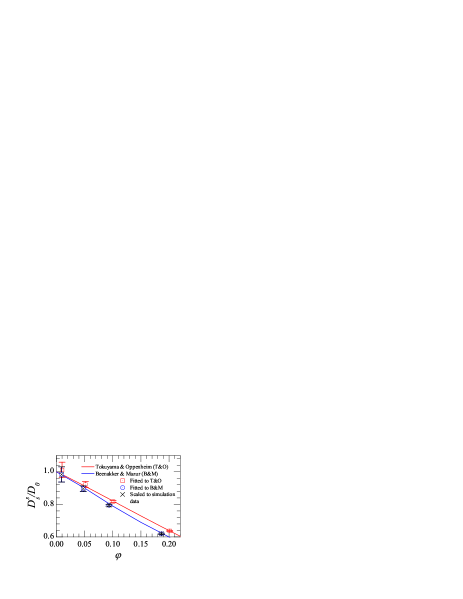
Figure 1: (Color online) Volume fraction dependence of the dimensionless short time self-diffusion coefficient. Open squares: experimental data with the absolute volume fraction scaled to fit the Tokuyama-Oppenheim prediction Tokuyama . Open circles: same data scaled to the Beenakker-Mazur prediction Beenakker . Crosses: same data scaled to maximize the overlap between the experimental and numerical results for the structural relaxation time, $\tau_{\alpha}$, in the glassy regime $\varphi\geq 0.55$. The scaling factor for absolute $\varphi$ between squares and circles is 1.07.

This calibration procedure can not be applied to our more polydisperse suspensions, since they do not crystallize. Instead, we calibrate the absolute $\varphi$ by comparing the volume fraction dependence of the short-time self-diffusion coefficient, $D_{s}$, to theoretical predictions by Tokuyama and Oppenheim Tokuyama and Beenakker and Mazur Beenakker . In practice, we start from an initial guess of the absolute volume fractions, $\varphi_{\rm guess}$, and measure $D_{s}$ vs. $\varphi_{\rm guess}$ in the range $\varphi_{\rm guess}\lesssim 0.2$ by fitting the initial decay of the ISF to $f(q,\tau\to 0)\simeq\exp(-q^{2}D_{s}\tau)$. As explained in Sec. II.3, we measure $f$ at $qR=4$ and under the best index matching conditions, to make sure that only the self part of the ISF is probed. We then fit $D_{s}(\varphi_{\rm guess})$ to the prediction for $D_{s}(\varphi)$ of either Ref. Tokuyama or Ref. Beenakker , setting $\varphi=b\varphi_{\rm guess}$. There are two fitting parameters in this procedure: $b$ is the scale factor for the absolute volume fractions, and $D_{0}\equiv\lim_{\varphi\to 0}D_{s}(\varphi)$ the self-diffusion coefficient in the limit of infinite dilution.

The results of the fit are shown in Fig. 1 together with the theoretical curves. The data agree well with both theoretical predictions, although the fit to the Beenakker-Mazur expression is slightly better. The ratio of the scaling factors $b$ obtained by fitting the data to Ref. Tokuyama or Ref. Beenakker , respectively, is 1.07. Thus, the spread in the estimate of the absolute volume fractions is of order 7%, comparable to that in Ref. vanmegen . Interestingly, the present method was used in Ref. SegrePRE1995 for a sample where calibration using the experimental freezing point was simultaneously possible, yielding fully compatible results.

As a final, alternative procedure to calibrate the absolute volume fraction, we compare our data for the equilibrium relaxation times described in more detail in Sec. IV below, to the results of Monte Carlo simulations for a three-dimensional binary mixture of hard spheres brambilla ; longtom . We find that it is possible to make data in the glassy regime coincide over about 5 decades of relaxation times by adjusting the experimental scale for $\varphi$ by a factor very close to that required to fit $D_{s}$ to the Beenakker-Mazur theory (see Fig. 1). In this paper, as in Ref. brambilla , we adopt for convenience the scaling factor required to collapse the experimental and numerical relaxation times in the glassy regime (crosses in Fig. 1).

This section shows that two distinct indicators obtained by theoretical and numerical work can be used to adjust absolute volume fractions in moderately polydisperse colloidal hard spheres, yielding results that are consistent within a confidence interval of about $\Delta\varphi/\varphi\approx 7~{}\%$, an uncertainty comparable to that plaguing adjustments onto the static phase diagram due to polydispersity effects. This uncertainty should be kept in mind when absolute numbers for critical volume fractions are compared between different works using different particles, different solvents, different techniques, and different calibrations for the volume fraction.

II.5 Data analysis

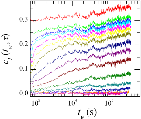
Figure 2: (Color online) Degree of correlation $c_{I}(t_{\mathrm{w}},\tau)$ measured for a sample with a volume fraction $\varphi=0.5970$. From top to bottom, the time delay $\tau$ is 0, 1, 10, 20, 50, 100, 200, 500, 1k, 2k, 5k, 10k, 20k, 50k, 100k, and 200k s. Note the logarithmic time axis, to better appreciate the initial aging regime.

As an example of the TRC data obtained in our experiments and their processing, we show in Figs 2 and 3 the degree of correlation $c_{I}$ and the final relaxation of the age-dependent ISF, respectively, for a sample at $\varphi=0.5970$. This is the densest system for which we were able to collect data at thermal equilibrium.

The degree of correlation initially grows with $t_{\mathrm{w}}$, implying that the change in sample configuration over a fixed time lag $\tau$ becomes progressively smaller, i.e. that the dynamics slows down. After about $10^{4}-10^{5}$ s the evolution of the dynamics essentially stops and a nearly stationary state is reached. Figure 3 shows the two-time ISF obtained by averaging the $c_{I}$ data of Fig. 2 over time windows of duration 200 s (for the younger ages) to 1000 s (for the oldest samples), for various ages $t_{\mathrm{w}}$ (for clarity, the fast dynamics measured with the goniometer apparatus is not shown). The lines are stretched exponential fits to the final decay of the ISF:

$$f(t_{\mathrm{w}},t_{\mathrm{w}}+\tau)=A(t_{\mathrm{w}})\exp\left\{-\left[\tau/\tau_{\alpha}(t_{\mathrm{w}})\right]^{p\,(t_{\mathrm{w}})}\right\}+B\,,$$ (6)

where $A$ is the height of the plateau preceding the final, or $\alpha$, relaxation, $\tau_{\alpha}$ the $\alpha$ relaxation time, $p$ the stretching exponent and $B\geq 0$ a small, residual base line most likely due to an imperfect correction of the effect of uneven illumination, as discussed in Ref. DuriPRE2005 . The aging behavior observed for $c_{I}$ in Fig. 2 is reflected by the increase of $\tau_{\alpha}$ with $t_{\mathrm{w}}$. We find that for $t_{\mathrm{w}}\geq 5\times 10^{4}$ s the relaxation time does not evolve any more (see also Fig. 6 and the related discussion below), while the height of the plateau still slightly increases, albeit extremely slowly. We take $t_{\mathrm{w}}=5\times 10^{4}$ as the end of the aging regime and obtain the equilibrium value of $\tau_{\alpha}$ as the average of the fitted relaxation time in the stationary regime.

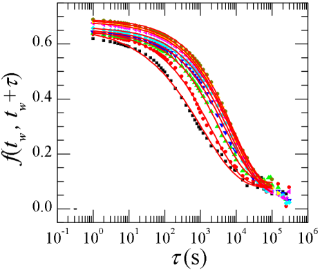
Figure 3: (Color online) Symbols: two-time intermediate scattering functions (ISFs) $f(t_{\mathrm{w}},t_{\mathrm{w}}+\tau)$ obtained from the degree of correlation shown in Fig. 2 ($\varphi=0.5970$). From left to right, $t_{\mathrm{w}}$ =1k, 2k, 5k, 10k, 50k, 100k, 200k, and 300k s. The solid lines are stretched exponential fits to the data according to Eq. (6).

III Measuring long relaxation times

We faced several challenges due to the extremely long relaxation times of the system, the use of a CCD detector, and the influence of gravity. In this section, we describe some of the potential artefacts and the difficulties associated with measurements on nearly glassy samples, together with our solutions to overcome these problems.

III.1 Sample heating and convection.

The CCD detector is much less sensitive than a traditional phototube or an avalanche photodiode. Consequently, a larger laser power is required, potentially leading to sample heating, if the particles or the solvent absorb light at the wavelength of the source. Under normal gravity conditions, local heating results in convective motion, which can significantly alter the spontaneous dynamics of our samples bellon . Figure 4 shows the age dependence of the $\alpha$ relaxation time obtained by fitting the ISF to Eq. (6), for a sample at $\varphi=0.5970$. The different curves are labeled by the power of the incident beam; when the largest available power is used (150 mW, full circles), $\tau_{\alpha}$ initially increases, as observed for many out-of-equilibrium systems, but then drops sharply with increasing $t_{\mathrm{w}}$. This surprising “rejuvenation” effect is much less pronounced when a reduced laser power is used (50 mW, open squares): the slowing down of the dynamics persists over a longer time span and the decrease of $\tau_{\alpha}$ that eventually sets in is more modest. These observations suggest that the acceleration of the dynamics, reported in one of our previous papers ElMasriJPCM2005 , is a non-linear effect perturbing the equilibrium dynamics, due to the onset of convective motion driven by sample heating. Indeed, we found that the solvent had became slightly yellowish since samples were prepared, which was responsible for increased absorption in the green region of the visible spectrum, where our laser operates.

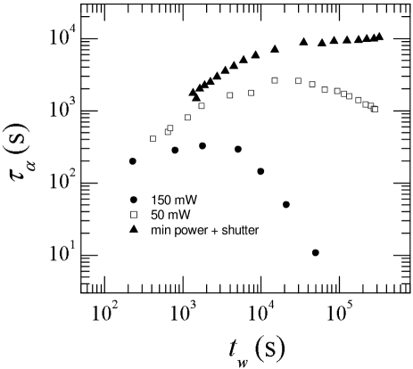
Figure 4: Age dependence of the $\alpha$ relaxation time for a sample at $\varphi=0.5970$. The curves are labeled by the laser power used for the measurement. The decrease of $\tau_{\alpha}$ at large $t_{\mathrm{w}}$ observed at the higher laser powers is an artefact due to sample heating and convection, which is removed by reducing the power and introducing a shutter.

To avoid any artefact due to convection, we have added a shutter to the setup, so that the sample is illuminated only for 100 ms at each CCD acquisition, rather than continuously. Since the typical acquisition rate is 1 Hz or lower, this reduces the average power injected in the sample by a factor of ten or more. Additionally, we perform our experiments at the minimum laser power compatible with a good beam stability (about 10 mW). Under these conditions, $\tau_{\alpha}$ is found to increase monotonically until a plateau is reached, with no rejuvenation effect even after 2 days, as shown by the triangles in Fig. 4. By changing the opening time of the shutter, we have checked that the dynamics shows no dependency on the average illuminating power, as long as the laser power is $\leq 10$ mW and the shutter time is $\leq 1$ s. As a final remark on this spurious rejuvenation, we note that this phenomenon sets in very slowly, especially when the laser power is not too high. This hints at a subtle interplay between aging and an external drive, similarly to the behavior of other soft glassy materials to which a (modest) mechanical perturbation is applied during their aging CoussotPRL2002 . More experiments will be needed to explore these analogies.

III.2 Sedimentation

Sedimentation is a potential additional source of a spurious acceleration of the dynamics, since it can act as a non-linear driving force. This is especially true for systems that relax very slowly and are very sensitive to external forcing sgr ; 2time . In the imaging geometry of our CCD setup, sedimentation results in an overall drift of the speckle pattern on the detector, which contributes to the change of $I_{p}$ at any given pixel and thus to the decay of $g_{2}$. We have implemented a correction scheme, which will be described in detail in a forthcoming publication; here we explain only the principles of the method. We use Image Correlation Velocimetry (ICV) TokumaruExpInFluids1995 , a technique similar to Particle Imaging Velocimetry, to measure the drift of the speckle pattern due to sedimentation for each pair of images taken at time $t_{\mathrm{w}}$ and $t_{\mathrm{w}}+\tau$. The drift is obtained by calculating the spatial crosscorrelation between the two speckle images. If the relative displacement of the particles over the lag $\tau$ is smaller than $1/q$, the lengthscale probed in a DLS experiment, the speckle pattern is essentially frozen, except for its overall drift. The second speckle image is then a shifted version of the first one; consequently, the crosscorrelation function exhibits a marked peak whose position corresponds to the average particle drift. Once the drift is obtained, the second image is back-shifted numerically NobachExpFluids2005 by the same amount but in the opposite direction, so as to compensate the physical drift. The corrected $c_{I}$ is finally calculated between the first image and the back-shifted version of the second one. The minimum shift that can be reliably measured is a few hundredths of a pixel, corresponding to about 50-100 nm in the sample. This is slightly less than $2\pi/q=250$ nm, the length scale over which the relative motion is probed by DLS: thus, we are able to detect and correct for an overall drift comparable to the relative displacement of the particles. Note that our correction method fails when the speckle pattern “boils” and changes faster than it drifts, since no peak in the crosscorrelation function can be detected reliably. However, this situations corresponds precisely to the case where the internal, spontaneous dynamics dominates over sedimentation, making the correction for the drift irrelevant.

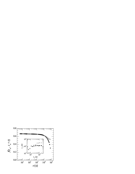
Figure 5: Main panel, filled squares: final relaxation of the ISF for a concentrated sample at $\varphi=0.5990$ and $t_{\mathrm{w}}=10^{5}$ s. The open symbols are the same data after correcting for the contribution of the average sedimentation velocity to the decay of $f$. Inset: for the same $\varphi$, $t_{\mathrm{w}}$ dependence of the $\alpha$ relaxation time for the raw ISFs and the corrected data.

Figure 5 shows both the raw (solid squares) and the corrected (open squares) $g_{2}-1$ for the most concentrated sample that we have studied ($\varphi=0.5990$) at $t_{\mathrm{w}}=10^{5}$ s. Sedimentation clearly affects the decay of $g_{2}$, which is about three times faster for the raw data than for the correct ones. The inset shows the large-age behavior of the relaxation time extracted from raw (open squares) and corrected (solid squares) correlation functions. Sedimentation leads to an apparent arrest of aging for $t_{\mathrm{w}}\geq 10^{4}$ s, while the corrected data indicate that the sample barely equilibrates for $t_{\mathrm{w}}\geq 10^{5}$, an age ten times larger. Note that, although we do correct for the average sedimentation velocity, we can not correct for velocity fluctuations stemming from hydrodynamics interactions and possibly changing the relative position of the particles, thereby contributing to the loss of correlation of the scattered light. Since velocity fluctuations are known to be relevant in concentrated suspensions NicolaiPhysFluids1995 , it is likely that sedimentation still accelerates to some extent the decay of $g_{2}$. These data are therefore not included in the analysis of equilibrium dynamics below.

It is interesting to compare the potential impact of sedimentation on our results to that in other works. A recent set of experiments SimeonovaPRL2004 on concentrated PMMA hard spheres has shown that aging is faster for off-buoyancy-matching particles than for nearly-buoyancy-matched colloids. Although our particles are not buoyancy-matched ($\Delta\rho=259~{}\mathrm{kg}\,\mathrm{m}^{-3}$), they are smaller than those used in the optical microscopy investigation of Ref. SimeonovaPRL2004 , enhancing the role of Brownian diffusion with respect to the gravity-driven drift. The relevant parameter is the inverse Peclet number

$$\Lambda=\frac{3k_{\mathrm{B}}T}{4\pi g\Delta\rho R^{4}}\,,$$ (7)

defined as the ratio of the gravitational length to the particle radius ($T$ is the absolute temperature and $k_{\mathrm{B}}$ the Boltzmann’s constant). In this work, $\Lambda\approx 870$, much larger than $\Lambda=44.1$ for the “normal gravity” experiments of Ref. SimeonovaPRL2004 (for which $\Delta\rho=300~{}\mathrm{kg}\,\mathrm{m}^{-3}$) and still greater than $\Lambda=678$ for their “reduced gravity” measurements ($\Delta\rho=20~{}\mathrm{kg}\,\mathrm{m}^{-3}$). Thus, our experiments are comparable to typical “reduced gravity” microscopy investigations. This illustrates the great advantage of using smaller particles to mitigate gravity effects, due to the $R^{-4}$ dependence of $\Lambda$. In order to further investigate the role of gravity in the slow dynamics of colloidal hard spheres in the large $\Lambda$ regime, light scattering measurements on small particles that are partially buoyancy-matched or microgravity experiments will be needed.

As a final remark on potential artefacts, one may wonder whether mechanical instabilities could be partially responsible for the ultra-slow decay observed in Fig. 5, where the relaxation time can be as large as 1.5 days. To test this possibility, we have measured $g_{2}$ for a sample compressed at random close packing and where very little dynamics is expected to occur. Although $g_{2}$ does exhibit some decay, whose origin is still unclear (either mechanical instability or some extremely slow rearrangement of the packed particles, or the contributions of a small number of “rattlers”), we stress that this relaxation is much slower than that observed for the most concentrated sample studied in this work. Furthermore, the relaxation of the most concentrated sample (Fig. 5) is a factor of 10 slower than the slowest equilibrium relaxation reported here and in Ref. brambilla : we can therefore rule out any significant artefact due to mechanical instability.

III.3 Non-equilibrium aging effects

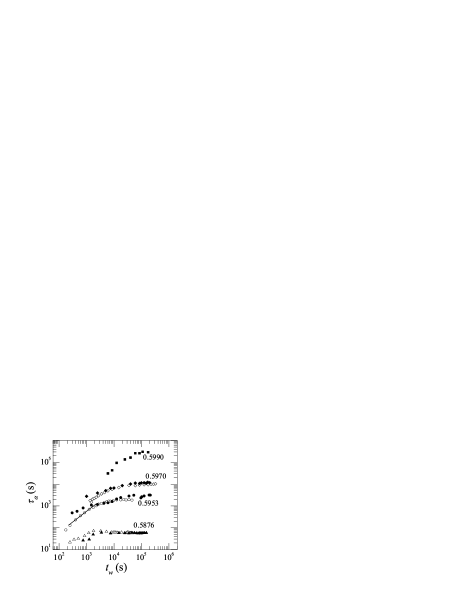
Figure 6: Age dependence of the $\alpha$ relaxation time for samples at volume fractions $0.5876\leq\varphi\leq 0.5990$, as indicated by the labels. Different symbol fillings correspond to independent experiments on the same sample. Large-$t_{\mathrm{w}}$ data for the two largest volume fractions are corrected for sedimentation effects. The line has a slope of one, showing that the initial growth of $\tau_{\alpha}$ is in general close to linear.

Besides artefacts due to sample heating and sedimentation, the dynamics of very concentrated samples become intrinsically difficult to measure, because of aging and dynamical heterogeneity. Aging is a quite general feature of glassy systems (see e.g. CipellettiJPCM2005 and references therein), where the dynamics slows down with time, or sample “age”, $t_{\mathrm{w}}$, as the system evolves towards equilibrium. In traditional DLS, the intensity correlation function has to be extensively averaged over time, making it impossible to capture the evolution of the dynamics for non-stationary systems. By contrast, the TRC approach and other multispeckle methods KirschJChemPhys1996 ; LucaRSI1999 ; ViasnoffRSI2002 allow one to fully characterize time-evolving dynamics, because the time average is replaced in part, or completely, by an average over the slightly different $q$ vectors associated to distinct pixels of the CCD.

Figure 6 shows the age dependence of $\tau_{\alpha}$ for samples prepared at different volume fractions $\varphi\geq 0.5876$. Symbols with the same shape but different filling correspond to independent experiments at the same volume fraction. Data for the two largest $\varphi$ are corrected for sedimentation effects at the largest $t_{\mathrm{w}}$; in all other cases, corrected and raw data yield the same results. Initially, $\tau_{\alpha}$ increases with $t_{\mathrm{w}}$; in this regime, the growth of $\tau_{\alpha}$ $vs.$ $t_{\mathrm{w}}$ is generally close to linear, as shown by the line $\tau_{\alpha}\propto t_{\mathrm{w}}$. For the most diluted sample in Fig. 6 ($\varphi=0.5876$), the initial aging regime is very short and is comparable to the time needed by the sample to equilibrate at the temperature imposed by the copper holder; consequently, no precise aging law can be determined. After the initial regime, $\tau_{\alpha}$ saturates and becomes almost independent of time, suggesting that all samples reach equilibrium, with the possible exception of the most concentrated suspension ($\varphi=0.5990$, squares in Fig. 6), for which the dynamics seem to keep slowing down over the full duration of the experiment (more than 3 days), although at an increasingly smaller rate. Note that the experiments are quite generally well reproducible, with the exception of the earliest stages, where presumably the dynamics is more influenced by the exact initial configuration and thermalization.

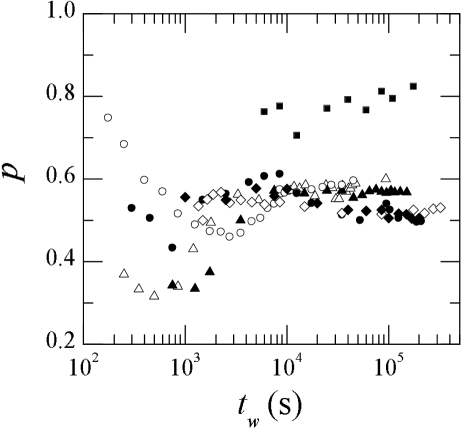
Figure 7: Age dependence of the stretching exponent $p$ obtained by fitting the final decay of the ISF to Eq. (6). Same symbols as in Fig. 6.

The time needed for reaching equilibrium, $t_{\mathrm{eq}}$, is about 30 times greater than the (equilibrium) relaxation time for the samples at the lowest volume fraction, $\varphi=0.5876$. However, this values is certainly overestimated due to the contribution of the thermalization time, of the order of $10^{3}$ s. For the samples at $\varphi=0.5953$ and $0.5970$, for which full equilibration is reached and where the initial thermalization time is negligible compared to all relevant time scales, $t_{\mathrm{eq}}/\tau_{\alpha}\approx 3-4$. This confirms the intuitive notion that equilibrium is reached on the time scale of a few structural relaxation times, i.e. after a few cage escape processes. Note that we are able to show that there is indeed an equilibrium regime even for samples whose $\alpha$ relaxation time is more than 7 orders of magnitude larger than that of very dilute suspensions. This significantly extends the range of samples that do reach equilibrium, compared to previous work vanmegen , where samples with $\tau_{\alpha}$ larger than $10^{5}$ times the Brownian decay time were classified as aging samples, most likely due to technical difficulties to access much larger relaxation timescales.

The time evolution of the stretching exponent $p(t_{w})$ is shown in fig. 7. For sufficiently large $t_{\mathrm{w}}$, $p$ saturates at 0.5-0.6, regardless of the volume fraction of the particles and the history of the samples. This stretched exponential shape might be related to sample polydispersity, since in previous experimental work on similar but less polydisperse colloidal hard spheres ($\sigma\approx 6\%$) the ISF was shown to relax nearly exponentially vanmegen . However, we point out that we find a similar value in the simulations described below in Sec. IV.2, for both $\sigma=5.77\%$ ($p\approx 0.55$) and $\sigma=11.5\%$ ($p\approx 0.65$). Interestingly, for the most concentrated sample $p$ remains well above the asymptotic value measured for all other samples, further suggesting that this sample has not fully relaxed during the experimental time window. Note that here we never observe “compressed” exponential relaxations ($p>1$), in contrast to the data of Ref. ElMasriJPCM2005 . We recall that for the latter laser heating yielded convection, which was most likely responsible for faster-than-exponential relaxations.

III.4 Dynamic heterogeneity

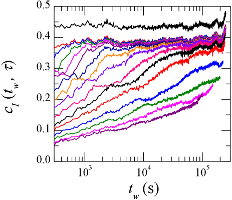
Figure 8: (Color online) Degree of correlation for the most concentrated sample ($\varphi=0.5990$). Note the large fluctuations of $c_{I}$, especially for $t_{\mathrm{w}}\leq 5\times 10^{3}$ sec, indicative of a temporally heterogeneous dynamics. From top to bottom, $\tau$ is 0, 5, 10, 25, 50, 100, 250, 1k, 2.5k, 5k, 10k, 25k, 50k, 100k, and 150k sec.

A detailed discussion of dynamical heterogeneity in samples at intermediate volume fractions ($0.20<\varphi<0.576$) has been presented in Refs. BerthierScience2005 ; brambilla ; dalleferrier . Here, we simply report that both the degree of correlation $c_{I}$ and the age-dependent ISF become more erratic and exhibit significant temporal fluctuations as $\varphi$ grows. An example is shown in Fig. 8 for $c_{I}$, and in Fig. 9 for the correspondent time-resolved ISFs. The data presented here are for the most concentrated sample that we have studied, $\varphi=0.5990$. Note that the fluctuations of $c_{I}$ are particularly relevant at early ages, when the sample is presumably farther from its equilibrium configuration. Because of these fluctuations, the shape of $f(t_{\mathrm{w}},t_{\mathrm{w}}+\tau)$ is less well defined, and the fits are generally poorer. However, we stress that $\tau_{\alpha}$ remains reasonably well defined, since the decay of the ISF, although somehow “bumpy”, is generally not too stretched, with the exception of the earliest ages.

The observation that $c_{I}$ and $f$ are increasingly noisy as $\varphi$ increases is consistent with the recently reported growth of cooperatively rearranging regions in supercooled colloidal suspensions approaching the glass transition WeeksScience2000 ; BerthierScience2005 ; brambilla ; WeeksJPCM2007 , in analogy with the behavior of molecular glass formers EdigerReview ; GlotzerReview . Indeed, as the size of the regions that rearrange cooperatively increases, the number of such regions in the scattering volume decreases: the dynamics are averaged over a smaller number of statistically independent objects, leading to enhanced fluctuations foampeter . The fact that dynamical fluctuations at high $\varphi$ are significant suggests that cooperatively rearranging regions may extend over a sizeable fraction of the scattering volume. This would imply a correlation length of the dynamics of the order of several hundreds of particle diameters, much larger than the $\sim 10$ particles reported in previous works WeeksScience2000 ; BerthierScience2005 ; brambilla ; WeeksJPCM2007 at lower $\varphi$, but comparable to recent findings in polydisperse colloids near random close packing BallestaNatPhys2008 . More experiments will be required to confirm these intriguing preliminary results.

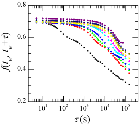
Figure 9: (Color online) Two-time ISFs obtained from the $c_{I}$ data shown in Fig. 8 ($\varphi=0.5990$). From left to right, $t_{\mathrm{w}}=500$, 5k, 7k, 10k, 20k, 30k, 50k, 70k, 100k, and 170k s. Dynamical heterogeneity at early times results in noisy ISFs, whose shape significantly departs from stretched exponential.

IV Analysis of equilibrium dynamics

IV.1 Equilibrium relaxation times

The first two sections were meant to convince the reader that it is possible to access the equilibrium dynamics of our colloidal hard sphere sample over a broad range of timescales for several well-controlled volume fractions. We now turn to the analysis of these results, which were briefly presented in a shorter paper brambilla .

In the inset of Fig. 10 we show the time decay of the ISF at selected volume fractions from a dilute system at $\varphi\approx 0.05$, up to very large volume fractions, $\varphi=0.597$ (same data as in Ref brambilla ). Our data cover a broad range of 11 decades in time, and we follow the slowing down of the equilibrium dynamics over about 7 decades in relaxation times.

In agreement with previous work pusey2 , we find that time correlation functions decay exponentially when volume fraction is moderate, with a time constant that increases weakly with $\varphi$. When $\varphi$ is increased above some ‘onset’ volume fraction, $\varphi\approx 0.5$, the relaxation becomes strongly non-exponential, with a two-step decay that become more pronounced as $\varphi$ continues to grow, signalling the arrest of particle motion for intermediate timescales. While the short-time decay is relatively unaffected by the increase of $\varphi$, the characteristic time of the second decay corresponding to the structural relaxation of the fluid increases rapidly over a small range of volume fraction. For $\varphi>0.597$, we were not able to collect data for which stationary behavior and thermal equilibrium could be unambiguously established, and this volume fraction marks thus the location of the ‘experimental colloidal glass transition’, $\varphi_{g}\approx 0.6$, by analogy with the temperature scale $T_{g}$ in thermal glasses. We do not attach any particular significance to $\varphi_{g}$, because it obviously depends on the details of the experimental set-up and of the sample.

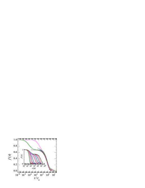
Figure 10: (Color online) Inset: representative ISFs for equilibrated samples at volume fractions 0.0480, 0.3096, 0.4967, 0.5555, 0.5772, 0.5818, 0.5852, 0.5916, 0.5957, 0.5970, from left to right. The lines are stretched exponential fits to the final decay of $f$. Main figure: scaling of the $\alpha$ relaxation of the ISFs for $\varphi\geq 0.4967$ when using the reduced variable $\tau/\tau_{\alpha}$. The line is the function $0.68\exp[-(\tau/\tau_{\alpha})^{0.558}]$.

As described in Sec. II.5, we fit the long-time decay of the time correlation functions to a stretched exponential form, Eq. (6). The resulting fits are shown in the inset of Fig. 10 as continuous lines. They describe the data very well and yield quantitative confirmation of the above qualitative remarks. We find that the amplitude $A$ of the decay is $A\approx 1$ at low $\varphi$ when relaxation is mono-exponential, so that $p\approx 1$ in that regime. When $\varphi$ increases, we find that $A$ drops to $A\approx 0.7$, signalling a two-step process. At the same time, the stretching exponent $p$ decreases and stabilizes around $p\approx 0.56$, indicating that structural relaxation occurs through a broad distribution of timescales.

The fact that $p$ is only weakly dependent on the volume fraction suggests that the structural decay of the ISFs should collapse when plotted against rescaled time, in the spirit of the ‘time temperature superposition principle’ frequently observed in molecular glass-formers. We show such a scaling in the main plot of Fig. 10, where the ISFs for $\varphi\geq 0.4967$ are plotted as a function of $\tau/\tau_{\alpha}$, with $\tau_{\alpha}$ the structural relaxation time issued from the stretched exponential fit to the data. The data collapse reasonably well onto a single master curve, confirming that the time volume fraction superposition principle holds for colloidal hard spheres, as observed in vanmegen .

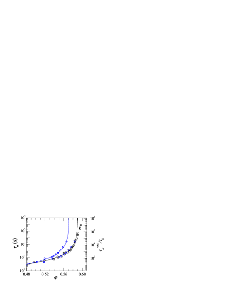
Figure 11: (Color online) Open squares, left axis: volume fraction dependence of the $\alpha$ relaxation timescale for equilibrated samples. The black line is an MCT fit to the data, Eq. (1). Open circles, right axis: $\alpha$ relaxation timescale measured by van Megen et al. in vanmegen , in units of the Brownian time, $\tau_{b}=Rr/(6D_{0})$. The blue line is an MCT fit to the data of vanmegen . Crosses: same data as the circles, plotted as a function of volume fraction scaled by a factor of 1.031, a value smaller than the uncertainty on $\varphi$ stated in vanmegen . The scaled data satisfactorily overlap with the measurement of this work.

We present in Fig. 11 the evolution of the equilibrium relaxation time $\tau_{\alpha}(\varphi)$ extracted from the fits of the ISFs. For the sake of clarity, only data for $\varphi\geq 0.48$ are shown: data at all volume fractions were reported in Ref. brambilla . While $\tau_{\alpha}$ increases by about 1 decade from $\varphi=0.05$ to $\varphi=0.5$ (data not shown), the structural relaxation slows down dramatically by about 6 decades when $\varphi$ approaches the largest volume fraction considered in this work. Following previous analysis vanmegen , we fit $\tau_{\alpha}$ to an algebraic divergence, as in Eq. (1), using $\varphi_{c}$ and $\gamma$ as adjustable parameters. Such a power law, predicted by MCT, cannot account for our data over the whole range of volume fraction, and the range of volume fractions fitted by Eq. (1) must be chosen with great care. As is also found in molecular glass-formers, we find that the power law Eq. (1) describes a window of relaxation times of about three decades, immediately following the onset of glassy dynamics, as shown in Fig. 11. The values of the exponent, $\gamma=2.5\pm 0.1$, and of the critical volume fraction, $\varphi_{c}=0.590\pm 0.005$, depend on the precise range of volume fraction fitted, but they agree well with previous work vanmegen , and theoretical and numerical analysis brambilla ; longtom , as we will further discuss in Sec. IV.3. If we attempt to include the largest volume fractions in our fit, we find that $\gamma$ takes unphysically large values, up to $\gamma\approx 6$. We interpret this finding as the sign that the growth of $\tau_{\alpha}$ is not appropriately described by Eq. (1) at large volume fraction.

A more direct indication can be observed in Figs. 10 and 11, since we were able to collect equilibrium data at volume fractions $\varphi$ above the fitted value of the critical volume fraction $\varphi_{c}$. Therefore, the dynamic singularity implied by Eq. (1) is not observed in our sample, and ergodic behavior can be detected for $\varphi>\varphi_{c}$. Just as is generically found in thermal glasses, we conclude therefore that the singularity predicted by mode-coupling theory is avoided in our experimental colloidal system. Although suggested by theory and computer simulations, such an observation was not reported in experimental work before.

As discussed in detail in Ref. brambilla , we find that an exponential divergence of $\tau_{\alpha}$ accounts for our data very well, as in Eq. (2). We argued in Ref. brambilla that the best fit of our data was obtained for $C=9.8\times 10^{-3}$, $\tau_{\infty}=6.5\times 10^{-3}$ sec, $\delta=2.0\pm 0.2$ and $\varphi_{0}=0.637\pm 0.002$, although imposing $\delta=1$, as in free volume predictions, yields an acceptable fit and a smaller critical volume fraction, $\varphi_{0}(\delta=1)=0.614\pm 0.002$.

Interestingly, the non-trivial exponent $\delta\approx 2$ is also supported by the numerical data for the polydisperse system of quasi-hard spheres studied in Sec. IV.2 (see Fig. 12 below), and by Monte Carlo results for a binary mixture of hard spheres brambilla ; longtom (also shown in Fig. 12). Additionally, a recent scaling analysis of the glass transition occurring in systems of soft repulsive particles yields $\delta=2.2\pm 0.2$ for the hard sphere limit longtom ; tom , a value compatible with that obtained here from the fit of Eq. (2). Thus, there is mounting evidence from both simulations and experiments that a simple VFT law, Eq. (2) with $\delta=1$, is not the most accurate description of the dynamics of hard spheres.

Overall, we find that while the onset of dynamical slowing can be described by an MCT divergence at a critical volume fraction $\varphi_{c}$, upon further compression a crossover from an algebraic to an exponential divergence at a much larger volume fraction $\varphi_{0}$ is observed, showing that the apparent singularity at $\varphi_{c}$ does not correspond to a genuine ‘colloidal glass transition’. Instead the system enters a regime where dynamics is ‘activated’, in the sense that $\tau_{\alpha}$ increases exponentially fast with the distance to $\varphi_{0}$. These observations therefore suggest that the glass transition scenario in colloidal hard spheres strongly resembles the one observed in molecular glass-forming materials.

IV.2 Polydispersity effects

A central finding from our experiments is the absence of a genuine dynamic singularity occuring at the fitted mode-coupling singularity $\varphi_{c}$. Since polydispersity influences the dynamics of colloidal hard spheres, we must ask how our findings may change for samples with a different polydispersity.

In Ref. vanmegen a sample less polydisperse than ours ($\sigma\approx 6\%$ as opposed to $\sigma\approx 10\%$) was analyzed using similar light scattering techniques, but no deviation from an algebraic singularity was reported. Additionally, experiments performed on samples at different polydispersities showed that increasing the polydispersity at constant volume fraction produces an acceleration of the dynamics poly . These observations suggest a possible explanation for our findings. One could argue that the observed ergodic behavior in our sample at large $\varphi$ stems from the fact that the glass state above the critical volume fraction $\varphi_{c}$ determined in Ref. vanmegen is ‘melted’ by polydispersity effects. In other words, polydispersity could push $\varphi_{c}$ to a much larger value so that our fluid states could all be observed below the “true” $\varphi_{c}$ characterizing our sample. This view is apparently supported by numerical analysis refRCPpolydisperse , which showed that volume fractions for the location of random close packing could be shifted from $\varphi_{\rm rcp}=0.64$ to $\varphi_{\rm rcp}=0.67$, from monodisperse to 10 % polydisperse samples, respectively, thus suggesting a similarly large shift in the MCT critical volume fraction.

This string of arguments is immediately contradicted by the fact that we have self-consistently determined $\varphi_{c}$ for our own sample, and that we do observe ergodic behavior for $\varphi$ which are larger than this critical volume fraction. It remains thus to establish that polydispersity does not qualitatively affect the dynamics in such a drastic manner that the results reported in this article do not shed light on the behavior of less polydisperse samples.

To definitely settle this issue, we performed computer simulations of a quasi-hard sphere system at different polydispersities DjamelPhD . Following previous work puertas , we study an assembly of point particles interacting via a purely repulsive potential:

$$V(r_{ij})=\epsilon\left(\frac{r_{ij}}{2R_{ij}}\right)^{36},$$ (8)

where $r_{ij}$ is the distance between particles $i$ and $j$, and $R_{ij}=(R_{i}+R_{j})/2$ with $R_{i}$ the radius of particle $i$. The prefactor $\epsilon$ is an energy scale. The interaction potential is very steep, and should therefore constitute a good approximation of the hard sphere potential. We set the polydispersity by drawing the particle radii from a flat distribution: $R_{i}\in[R-\delta R/2,R+\delta R/2]$, so that the average diameter is $\overline{R_{i}}=R$ and the polydispersity is $\sigma=\sqrt{\overline{R_{i}^{2}}-R^{2}}/R=\delta R/(\sqrt{12}R)$. We have studied the system for two values of polydispersity, $\delta R/R=0.2$ and 0.4, leading to polydispersities $\sigma\simeq 5.77~{}\%$ and $\sigma\simeq 11.5~{}\%$, which compare well with the colloidal samples studied in Ref. vanmegen and in the present study, respectively.

We follow previous work dedicated to the Hamiltonian (8) in the context of hard spheres. We solve Newton’s equations for $N$ particles of mass $m$ inside a three-dimensional simulation box of size $L$ with periodic boundary conditions allen . For the inverse power law potential in Eq. (8), density and temperature can be combined in a unique control parameter, $\Gamma=\varphi T^{-1/12}$, so we fix the temperature and energy scales, $k_{B}T=\epsilon=1/3$, and vary the system size to change the volume fraction, $\varphi=4\pi NR^{3}[1+(\delta R/4R)^{2}]/(3L^{3})$. Since we deal with soft spheres, it is of course not possible to compare absolute values for critical volume fractions with results obtained in the true hard sphere limit. Timescales are expressed in units of $2R\sqrt{m/\epsilon}$. We choose the self-intermediate scattering function $F_{s}(q,t)$ as a dynamic observable, and work at a single wavevector, $qR=3.9$, close to the first diffraction peak.

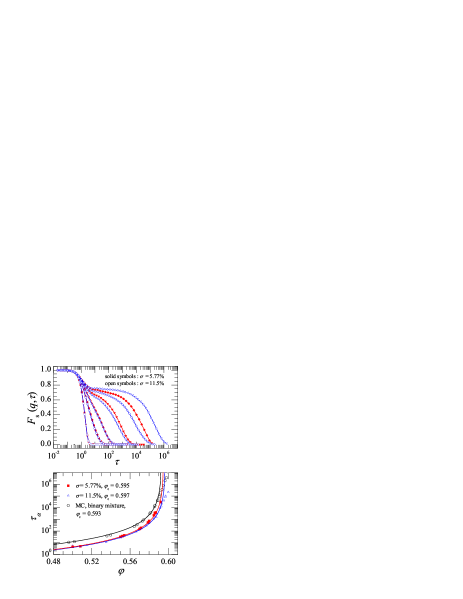
Figure 12: (Color online) Top panel: self-intermediate scattering function from numerical simulations of a quasi-hard sphere system at two different values of the polydispersity, $\sigma$, and various volume fractions. For the less polydisperse system, $\varphi=0.053$, 0.50. 0.55, 0.58 and 0.592, from left to right. For the more polydisperse system, $\varphi=0.074$, 0.50, 0.55, 0.58, 0.5914 and 0.60, from left to right. Bottom panel : relaxation time $\tau_{\alpha}$ for the two systems, with data from Monte Carlo simulations of a binary mixture brambilla superimposed. The three sets of data are fitted to the MCT prediction, Eq.(1), using the same exponent $\gamma=2.7$. The critical volume fraction issued from the fit is shown in the label.

We perform the simulations in two steps. We prepare initial configurations at the desired state points, and perform a long equilibration run using periodic velocity rescaling to reach thermal equilibrium. We then perform a production run in the microcanonical ensemble. We check very carefully that thermal equilibrium is indeed reached during equilibration. We also check that our results do not depend on the duration of these two steps, and we repeat them for at least five independent samples at each volume fraction to obtain better statistics. The main issue, mentioned in the original work of Ref. puertas , is the possibility for the less polydisperse system ($\sigma\approx 6\%$) to crystallize in the course of the simulation. In this case the sample is discarded and a new sample studied. We found that this problem is much more severe than reported in Ref. puertas , and so we were not able to collect data above $\varphi=0.587$. For the more polydisperse system ($\sigma\approx 12\%$), we never detected crystallization and we were able to collect data up to $\varphi=0.60$, where we stopped because we could not reach equilibrium within our numerical time window. It is interesting to note that crystallization similarly prevented the colloidal samples of Ref. vanmegen to be studied at very large volume fractions, while no such problem is encountered for the colloidal system studied in this article.

We report in the top panel of Fig. 12 some representative results for the self-intermediate scattering function of the system at two polydispersities, and different volume fractions. This figure is qualitatively very similar to the experimental data of Fig. 10, with a pronounced non-exponential relaxation which slows down dramatically when $\varphi$ increases. When volume fraction is low, we see that the change in polydispersity has no detectable influence on the dynamics, and data for the two systems nicely superimpose. A first visible effect of polydispersity is that we do not have data for the 6 % polydisperse sample at very large values of the relaxation time because the system eventually crystallizes. A second effect can be detected when the glassy regime is entered. For a fixed $\varphi$, the dynamics of the system become faster when polydispersity is increased, as observed previously poly ; sear .

To quantify these observations, we fit the long time decay of the relaxation to a stretched exponential form, as in Eq. (6), and show the results for $\tau_{\alpha}(\varphi)$ in the bottom panel of Fig. 12. As mentioned before, the polydispersity has very little effect when dynamics is fast, $\varphi<0.5$, while the more polydisperse sample relaxes faster in the glassy regime.

We have fitted the dynamic slowing down with increasing $\varphi$ to the algebraic form suggested by MCT. As expected, we find that polydispersity affects the value of the critical volume fraction, although the change is rather modest, since $\varphi_{c}$ increases from $\varphi_{c}=0.595$ to $\varphi_{c}=0.597$ when changing polydispersity from 6 % to 12 %. Note that we used the same exponent $\gamma=2.7$ to fit both sets of data over a comparable window of relaxation times, showing that polydispersity does not quantitatively affect the form of the slowing down. It must be noted that the shift in the absolute value of $\varphi_{c}$ is much less severe than expected from that for the random close packing volume fraction on the basis of the numerical work of Ref. refRCPpolydisperse .

It is interesting to note that deviations from the MCT power law cannot be detected very clearly for the less polydisperse system, because crystallization prevents observation of larger relaxation timescales. For the more polydisperse system, however, we find that deviations from the MCT power law at even larger volume fractions become observable, since a broader window of relaxation timescales can be measured. We believe that similar effects are relevant also in experiments. As we will show shortly, both the experiments reported in Ref. vanmegen and our data are described by a comparable power law over a similar window of relaxation timescales. However, while previous work did not detect deviations from an algebraic divergence, by studying a more polydisperse system, we can efficiently suppress crystallization and access a range of equilibrium relaxation timescales that are beyond the volume fraction regime which can be described by MCT, but the MCT regime itself is not qualitatively affected by polydispersity effects.

For completeness, we report in the bottom panel of Fig. 12 the Monte Carlo results obtained in Ref. brambilla for a three-dimensional 50:50 binary mixture of hard spheres of diameter ratio 1.4, for which polydispersity is $\sigma\approx 16.7~{}\%$. Again, we find that the data is qualitatively unaffected by the use of a very different particle size distribution, by the fact that a true hard sphere potential is used, and by the use of a stochastic microscopic dynamics. An MCT power law also describes the data over a comparable time window of about three decades, with a similar exponent $\gamma=2.7$, and a critical volume fraction $\varphi_{c}=0.593$. Remember that we cannot directly compare the result for $\varphi_{c}$ to the ones for the quasi-hard sphere system, since the latter is dependent on the temperature scale used (a larger temperature would yield a smaller critical density). Overall, it is reassuring that whenever comparison is possible, neither the choice of a microscopic dynamics, nor the particle size distribution and polydispersity seem to influence the dynamics in a drastic manner. This certainly suggests that quantitative comparison between different experimental samples is meaningful.

IV.3 Comparison with previous work

Considering colloidal hard spheres from the viewpoint of the glass transition field, it is very natural to expect, just as is found for all molecular glasses, that the dynamic singularity deduced from fitting data to an algebraic law predicted by MCT is eventually avoided as the glassy regime is entered more deeply. Yet, the present experiment is the first direct demonstration that the MCT dynamic transition is avoided in a colloidal hard sphere sample. Although we are tempted to assume that our conclusions should apply to all colloidal hard spheres samples, this statement would seem to require additional discussion.

First, it is reassuring to observe that several computational studies performed in recent years with hard spheres, using different types of polydispersities, and different types of microscopic dynamics indicated the presence of strong deviations from an algebraic divergence when approaching $\varphi_{c}$. In that sense, the experiments of Ref. vanmegen stood as an exception, although arguably an important one.

In Fig. 11, we report data from Ref. vanmegen ($\tau_{\alpha}^{\mathrm{vM}}$, blue circles and crosses and right axis), together with our data, taken from Ref. brambilla ($\tau_{\alpha}$, black squares and left axis). The open circles are the data as presented in Ref. vanmegen , using $\varphi$ values that may be underestimated by a factor $\leq 1.04$, because of polydispersity, as discussed in Sec. II.4. An MCT fit to $\tau_{\alpha}^{\mathrm{vM}}(\varphi)$ yields $\varphi_{\mathrm{c}}=0.572\equiv\varphi_{\mathrm{c}}^{\mathrm{vM}}$ vanmegen (blue line). The crosses are the same data plotted against volume fraction scaled by a factor $\varphi_{\mathrm{c}}/\varphi_{\mathrm{c}}^{\mathrm{vM}}=1.031$, with $\varphi_{\mathrm{c}}=0.59$ the critical volume fraction obtained by fitting our data to the MCT prediction, Eq. (1) noteshifttime . Note that the scaling factor required for the MCT critical volume fractions to coincide is smaller than the uncertainty in the absolute $\varphi$ for both sets of data. When compared over the range of volume fraction where MCT applies, both sets of data are nearly indistinguishable, confirming that in this regime sample polydispersity has a very small influence on the dynamics, as indicated by the simulations discussed in Sec. IV.2.

Figure 11 shows also that the range of timescales reported in Ref. vanmegen is relatively smaller by about two decades than the present data. Assuming that the behavior of the fluid at larger $\varphi$ for the sample of Ref. vanmegen would also compare well with the one we observe, one realizes that the data point of Ref. vanmegen at the highest $\varphi$ lies just below the volume fraction where deviations from MCT predictions should start becoming visible, possibly explaining why no such deviations were observed in that work. Of course, obtaining equilibrium data at larger $\varphi$ for this sample would be difficult, because slow dynamics would start competing with crystallization, as we observed numerically in Sec. IV.2 for the sample at the lowest polydispersity.

V Conclusions

We have discussed some of the challenges that must be faced when investigating the slow dynamics of concentrated colloidal systems, together with the solutions we devised. These challenges include the determination of the absolute volume fraction and avoiding or at least minimizing artefacts due to sedimentation and convection. At very large volume fractions, aging and dynamical heterogeneity make measurements even more difficult. The data become more erratic, suggesting that a proper ensemble average is not being achieved.

The data presented here and in brambilla show unambiguously that, for our sample, the power-law divergence of $\tau_{\alpha}(\varphi)$ is avoided and that at high $\varphi$ the growth of the relaxation time is well described by a generalized VFT law. A comparison with the measurements reported by van Megen et al. vanmegen indicates that, in the MCT regime, the two sets of data are compatible within the experimental uncertainty on the absolute volume fraction. This suggests that the slow dynamics of hard spheres is only weakly sensitive to the precise value of polydispersity, at least up to moderate values $\sigma~{}\sim 10\%$. Our numerical work supports this conclusion. The agreement between our data and previous work strongly suggests that the absence of a true algebraic divergence of $\tau_{\alpha}$ should be a general feature in colloidal hard spheres, independent of the details of the system. In this respect, hard spheres should be similar to molecular glass formers, for which the MCT transition is avoided as well.

Several questions remain open. While we were able to rule out the existence of an MCT glass transition at $\varphi=\varphi_{\mathrm{c}}\approx 0.59$, our experiments do not allow us to determine unambiguously whether the location of the divergence of $\tau_{\alpha}$ obtained by a generalized VFT fit, $\varphi_{0}=0.637$, is distinct from $\varphi_{\mathrm{rcp}}$. Addressing this issue would allow one to discriminate between competing theoretical approaches jorge , e.g. recent excluded volume approaches ken and thermodynamic glass transition theories silvio ; zamponi . However, providing an experimental answer will be particulary difficult: on one hand, $\varphi_{0}$ can only be obtained by extrapolation. On the other hand, $\varphi_{\mathrm{rcp}}$ is difficult to locate both on a conceptual standpoint torquato2 and because any deviations from the behavior of an ideal hard sphere potential may become important very close to $\varphi_{\mathrm{rcp}}$.

Another promising line of research concerns the aging regime. We have shown that at the highest volume fractions investigated the dynamics slows down over a period of the order of a few (equilibrium) structural relaxation times. Whether a similar behavior also applies to more diluted samples remains to be ascertained. Indeed, in our experiments the thermalization time, during which convective motion is likely to set in due to small temperature gradients across the sample, was too long to reach any conclusive result for $\varphi<0.5953$. The large dynamical heterogeneity of the most concentrated sample suggests that dynamical fluctuations may be much larger than previously thought in out-of-equilibrium samples at very high $\varphi$. The interplay between dynamical heterogeneity and the evolution of the dynamics in the aging regime appears as a promising field for future investigation.

- (1) W. B. Russel, D. A. Saville, and W. R. Schowalter, Colloidal dispersions (Cambridge University Press, Cambridge, 1992).
- (2) P. Habdas and E. R. Weeks, Current Opinion in Colloid & Interface Science 7, 196 (2002).
- (3) B. J. Berne and R. Pecora, Dynamic Light Scattering (Wiley, New York, 1976).
- (4) P. N. Pusey and W. van Megen, Nature 320, 340 (1986).
- (5) W. C. K. Poon, J. Phys.: Condens. Matter 14, R859 (2002).
- (6) S. C. Glotzer and M. J. Solomon, Nature Materials 6, 557 (2007).
- (7) W. K. Kegel, Langmuir 16, 939 (2000).
- (8) N. B. Simeonova and W. K. Kegel, Phys. Rev. Lett. 93, 035701 (2004).
- (9) G. Brambilla, D. El Masri, M. Pierno, G. Petekidis, A. B. Schofield, L. Berthier, and L. Cipelletti, Phys. Rev. Lett. 102, 085703 (2009).
- (10) W. Götze, J. Phys.: Condens. Matter 11, A1 (1999).
- (11) W. van Megen, T. C. Mortensen, S. R. Williams, J. Müller, Phys. Rev. E 58, 6073 (1998).
- (12) P. N. Pusey, and W. Van Megen, Phys. Rev. Lett. 59, 2083 (1987).
- (13) T. G. Mason and D. A. Weitz, Phys. Rev. Lett. 75, 2770 (1995).
- (14) P. N. Pusey, and W. Van Megen, Nature 320, 595 (1986).
- (15) M. H. Cohen and D. Turnbull, J. Chem. Phys. 31, 1164 (1959).
- (16) K. S. Schweizer, J. Chem. Phys. 127, 164506 (2007).
- (17) M. Cardenas, S. Franz, and G. Parisi, J. Chem. Phys. 110, 1726 (1999).
- (18) G. Parisi and F. Zamponi, J. Chem. Phys. 123, 144501 (2005).
- (19) Z. Cheng, J. Zhu, P. M. Chaikin, S. Phan, and W. B. Russel, Phys. Rev. E 65, 041405 (2002).
- (20) S. K. Kumar, G. Szamel, and J. F. Douglas, J. Chem. Phys. 124, 214501 (2006).
- (21) P. G. Debenedetti and F. H. Stillinger, Nature 410, 259 (2001).
- (22) C. S. O’Hern, S. A. Langer, A. J. Liu, and S. R. Nagel, Phys. Rev. Lett. 88 075507 (2002).
- (23) S. Torquato, T. M. Truskett, and P. G. Debenedetti, Phys. Rev. Lett. 84, 2064 (2000).
- (24) L. Berthier and T. A. Witten, arXiv:0903.1934.
- (25) T. R. Kirkpatrick, D. Thirumalai, and P. G. Wolynes, Phys. Rev. A 40, 1045 (1989).
- (26) J.-P. Bouchaud and G. Biroli, J. Chem. Phys. 121, 7347 (2004).
- (27) S.-E. Phan, W. B. Russel, Z. Cheng, J. Zhu, P. M. Chaikin, J. H. Dunsmuir, R. H. Ottewill, Phys. Rev. E 54, 6633 (1996).
- (28) S. P. Das and G. F. Mazenko, Phys. Rev. A 34, 2265 (1986).
- (29) M. E. Cates and S. Ramaswamy, Phys. Rev. Lett. 96, 135701 (2006).
- (30) A. Andreanov, G. Biroli, and A. Lefèvre, J. Stat. Mech. P07008 (2006).
- (31) G. Szamel and E. Flenner, Europhys. Lett. 67, 779 (2004).
- (32) L. Berthier and W. Kob, J. Phys.: Condens. Matter 19, 205130 (2007).
- (33) L. Berthier, Phys. Rev. E 76, 011507 (2007).
- (34) P. N. Pusey, J. Phys. A 11, 119 (1978); P. N. Pusey, H. M. Fijnaut, and A. Vrij, J. Chem. Phys. 77, 4270 (1982).
- (35) W. Schaertl and H. Sillescu, J. Stat. Phys. 74, 1007 (1994).
- (36) D. El Masri, M. Pierno, L. Berthier, and L. Cipelletti, J. Phys.: Condens. Matter 17, S3543 (2005).
- (37) L. Cipelletti, H. Bissig, V. Trappe, P. Ballesta, and S. Mazoyer, J. Phys.: Condens. Matter 15, S257 (2003).
- (38) A. Duri, H. Bissig, V. Trappe, and L. Cipelletti, Phys. Rev. E 72, 051401 (2005).
- (39) J. Z. Xue, D. J. Pine, S. T. Milner, X. L. Wu, and P. M. Chaikin, Phys. Rev. A 46, 6550 (1992).
- (40) J. W. Goodman, in Laser speckles and related phenomena, edited by J. C. Dainty (Springer-Verlag, Berlin, 1975), Vol. 9, p. 9.
- (41) M. Tokuyama, and I. Oppenheim, Phys. Rev. E 50, R16 (1994).
- (42) C. W. J. Beenakker and P.Mazur, Physica A 120 388 (1983).
- (43) P. N. Segre, O. P. Behrend, and P. N. Pusey, Phys. Rev. E 52, 5070 (1995).
- (44) L. Bellon, M. Gibert, and R. Hernandez, Eur. Phys. J. B 55, 101 (2007).
- (45) P. Coussot, Q. D. Nguyen, H. T. Huynh, and D. Bonn, Phys. Rev. Lett. 88, (2002).
- (46) P. Sollich, F. Lequeux, P. Hebraud, and M. E. Cates, Phys. Rev. Lett. 78, 2020 (1997).
- (47) L. Berthier, J.-L. Barrat, and J. Kurchan, Phys. Rev. E 61, 5464 (2000).
- (48) P. T. Tokumaru and P. E. Dimotakis, Experiments in Fluids 19, 1 (1995).
- (49) H. Nobach, N. Damaschke, and C. Tropea, Experiments in Fluids 39, 299 (2005).
- (50) H. Nicolai, B. Herzhaft, E. J. Hinch, L. Oger, and E. Guazzelli, Physics of Fluids 7, 12 (1995).
- (51) L. Cipelletti and L. Ramos, J. Phys.: Condens. Matter 17, R253 (2005).
- (52) S. Kirsch, V. Frenz, W. Schartl, E. Bartsch, and H. Sillescu, J. Chem. Phys. 104, 1758 (1996).
- (53) L. Cipelletti and D. A. Weitz, Rev. Sci. Instrum. 70, 3214 (1999).
- (54) V. Viasnoff, F. Lequeux, and D. J. Pine, Rev. Sci. Instrum. 73, 2336 (2002).
- (55) L. Berthier, G. Biroli, J. P. Bouchaud, L. Cipelletti, D. El Masri, D. L’Hote, F. Ladieu, and M. Pierno, Science 310, 1797 (2005).
- (56) C. Dalle-Ferrier, C. Thibierge, C. Alba-Simionesco, L. Berthier, G. Biroli, J.-P. Bouchaud, F. Ladieu, D. L’Hôte, and G. Tarjus, Phys. Rev. E 76, 041510 (2007).
- (57) E. R. Weeks, J. C. Crocker, A. C. Levitt, A. Schofield, and D. A. Weitz, Science 287, 627 (2000).
- (58) E. R. Weeks, J. C. Crocker, and D. A. Weitz, J. Phys.: Condens. Matter 19, (2007).
- (59) M. D. Ediger, Annu. Rev. Phys. Chem. 51, 99 (2000).
- (60) S. C. Glotzer, J. Non-Cryst. Solids 274, 342 (2000).
- (61) P. Mayer, H. Bissig, L. Berthier, L. Cipelletti, J.P. Garrahan, P. Sollich, and V. Trappe, Phys. Rev. Lett. 93, 115701 (2004).
- (62) P. Ballesta, A. Duri, and L. Cipelletti, Nature Physics 4, 550 (2008).
- (63) L. Berthier and T. A. Witten, arXiv:0810.4405.
- (64) S. R. Williams and W. van Megen, Phys. Rev. E 64, 041502 (2001).
- (65) D. El Masri, PhD thesis, Université Montpellier 2 (2007).
- (66) T. Voigtmann, A. M. Puertas, and M. Fuchs, Phys. Rev. E 70, 061506 (2004).
- (67) M. Allen and D. Tildesley, Computer Simulation of Liquids (Oxford University Press, Oxford, 1987).
- (68) R. P. Sear, J. Chem. Phys. 113, 4732 (2000).
- (69) F. Krzakala and J. Kurchan, Phys. Rev. E 76, 021122 (2007).
- (70) A shift factor on the axis was used to match the datasets. This factor accounts for the differences in particle size, solvent viscosity, vector and definition of in the two experiments.