A Conformal Field Theory for Eternal Inflation

Ben Freivogel and Matthew Kleban

¹ Berkeley Center for Theoretical Physics, Department of Physics
University of California, Berkeley, CA 94720-7300, USA
and
Lawrence Berkeley National Laboratory, Berkeley, CA 94720-8162, USA

²Center for Cosmology and Particle Physics

Department of Physics, New York University

4 Washington Place, New York, NY 10003.

We study a statistical model defined by a conformally invariant distribution of overlapping spheres in arbitrary dimension $d$. The model arises as the asymptotic distribution of cosmic bubbles in $d+1$ dimensional de Sitter space, and also as the asymptotic distribution of bubble collisions with the domain wall of a fiducial “observation bubble” in $d+2$ dimensional de Sitter space. In this note we calculate the 2-,3-, and 4-point correlation functions of exponentials of the “bubble number operator” analytically in $d=2$. We find that these correlators are free of infrared divergences, covariant under the global conformal group, charge conserving, and transform with positive conformal dimensions that are related in a novel way to the charge. Although by themselves these operators probably do not define a full-fledged conformal field theory, one can use the partition function on a sphere to compute an approximate central charge in the 2D case. The theory in any dimension has a noninteracting limit when the nucleation rate of the bubbles in the bulk is very large. The theory in two dimensions is related to some models of continuum percolation, but it is conformal for all values of the tunneling rate.

1 Introduction

De Sitter space plays a central role in cosmology. In the standard model, the first moment after the big bang was a period of inflation in which the universe expanded many times over during an approximately de Sitter phase. Recent observations indicate that the expansion is currently accelerating, indicating the presence of a dark matter component which is most economically explained by a positive cosmological constant—in which case the future of our universe is a de Sitter phase. Moreover, if string theory is the correct description of nature, we may expect that our entire observable universe is a bubble expanding in an eternally inflating false vacuum de Sitter space [1, 2]. In such a model bubbles of the true vacuum nucleate in the false vacuum, and their walls accelerate outwards under the gravitational pressure due to the differing values of the vacuum energy inside and out. Observers may form inside these cosmic bubbles, which viewed from the inside appear to be negatively curved expanding Robertson-Walker cosmologies [3]. The cosmology inside will be affected in interesting ways both at its “Big Bang” [4] and later, by collisions with other bubbles (see e.g [5]). If this model is correct, understanding de Sitter space becomes even more crucial.

But de Sitter space has proved maddeningly difficult to understand. In eternal de Sitter, points at fixed comoving distance always become causally disconnected at late times. As a result, correlation functions of points separated by more than a single Hubble length are not observable, and so one cannot define observables (like an S-matrix or boundary correlation functions in anti-de Sitter space) using well-separated points in space [6]. Moreover, because of the thermal nature of de Sitter and its finite entropy one expects correlators of operators inserted at timelike separated points to be quasi-periodic functions of the time separation, which neither converge nor settle into any predictable pattern (and in fact eventually produce fluctuations to every state consistent with the conservation laws) [7, 8]. Attempts to define a dS/CFT correspondence indicate that if such a dual theory exists, it cannot be unitary [9, 10]. In the larger “multiverse” of the string theory landscape, one would like to understand how to average over distributions of cosmic bubbles so as to compute the expected values of cosmological observables visible to those living inside them. Much interesting work has been done on this problem; see e.g [11] for a review. However, this too has been plagued by infinities and the non-uniqueness in the choice of measure.

Here, we analyze the correlation functions of a putative dual CFT for eternal inflation. Our philosophy is that if one can find a consistent and well-defined set of quantities in eternally inflating spaces, this may lead to a solution of many of the problems above. To begin, consider an eternally inflating spacetime in $d+1$ spacetime dimensions in which at least one interacting scalar field is undergoing tunneling and forming bubbles. If one takes a $d$-dimensional constant time slice across the spacetime at late time, the slice will contain many casually disconnected regions and many vacuum bubbles, as shown in figures 1 and 2. Each bubble appears initially with small size, but as time passes its radius grows, asymptoting to a finite comoving radius determined by the conformal time at which it appeared (late appearing bubbles are smaller).

We make some simplifying assumptions which allow us to compute the statistical distribution of these bubbles on the $d$-slice. (For a more general discussion, see [13].) This approach has the advantage of simplicity, but the disadvantage that these bubble distributions are not observable.

Any given observer can observe only a subset of the eternally inflating spacetime. Consider an observer inside a bubble of some type, the “observation bubble.” The observation bubble collides with other bubbles that form through quantum nucleation in the false vacuum nearby, as shown in figure 1. Each collision bubble will affect the observation bubble’s wall inside a ball (a disk in the case of an observer 3+1 dimensional de Sitter). As time passes for an observer inside the observation bubble the collision appears as a point and grows at a rate which asymptotically approaches that of the observation bubble’s wall itself. As a result the angular radius of the disk asymptotes at late time to some finite size $\psi$, which is determined in a simple way by the time of the collision (late collisions make smaller disks). If the observer has access to large conformal times—which requires that the cosmological constant inside the observation bubble be small—she can observe this asymptotic distribution by, for example, its effects on her cosmic microwave background sky. Such an observer has been referred to as a “census taker” [12].

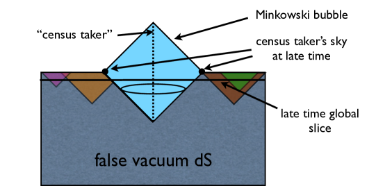
Figure 1: A Carter-Penrose conformal diagram for bubbling de Sitter space. One can slice with a constant global time surface, which from $d=2+1$ de Sitter would produce a 2-sphere tiled with bubbles (see Fig. 2). Alternatively one can consider the sky as observed at late times by a “census taker” living in a $\Lambda=0$ bubble. Starting from $d=3+1$ de Sitter, this will produce a very similar 2-sphere.

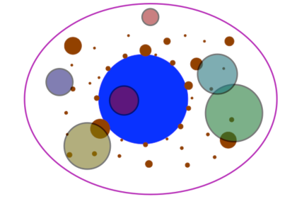
Figure 2: Artist’s rendition of a global slice of bubbling de Sitter space at late times, or a census taker’s sky.

We will investigate the statistics of the distribution of these bubbles and their collisions, focusing primarily on the case of 2D distributions. The distribution can be thought of as describing either the set of bubbles on a late time slice in 2+1 dimensional de Sitter space, or the set of collisions with an observation bubble in 3+1 de Sitter. As we will see, using the bubble distribution on these surfaces one can define a set of correlation functions which behave like primary operators of a 2D conformal field theory. The operators are the exponentials of a discrete number operator that counts the number of disks that overlap the point where it is inserted.

Using the distribution we compute the 2–,3–, and 4-point functions of these exponential operators analytically and exactly. These turn out to be consistent with the hypothesis that these exponential operators are primary fields of a conformal field theory, except that the 4-point function exhibits a non-analyticity as a function of the location of the operator insertions. The theory is conformally invariant for arbitrary values of the dimensionless tunneling rate $\gamma$. The relation between the charge $\beta$ of the exponential of the number operator $e^{i\beta N(z)}$ and its scaling dimension is interesting and novel:

$$\Delta\left(\beta\right)=\pi\gamma(1-\cos\beta).$$ (1.1)

We compute the central charge of this putative conformal field theory by evaluating its partition function on a sphere of radius $R$, and find a result proportional to the continuous parameter $\gamma$.

We also discuss higher dimensional versions of the theory. The simplest such extension is a 3D version obtained from the statistics of bubbles on 3D global slices of $3+1$ de Sitter. This 3D theory has a dimension zero number operator, and its exponentials again behave like primary fields with positive dimension. In fact, we can show that in any dimension $d$, the theory always contains a dimension zero number operator and exponential operators constructed from it with arbitrarily small positive weight. Since no such operator can exist in a unitary field theory in more than $d=2$, these higher dimensional theories cannot be unitary.

Finally, we will demonstrate that in the limit that the decay rate $\gamma\to\infty$, the theory in any number of dimensions becomes free: correlators of the exponential operators factorize onto products of 2-point functions in precisely the same way as vertex operators for a free, massless scalar in two dimensions.

2 Conformal invariance

The simplest case to consider is one in which the cosmological constant inside the bubbles is the same as that of the “false vacuum” outside, and where bubbles can nucleate both inside and outside other bubbles—always with the same decay rate $\gamma$, where $\gamma$ is defined as the dimensionless decay rate per unit Hubble time per unit Hubble volume.

In order for the tunneling rate to be constant, all of the vacua should be identical. The simplest model is the potential drawn in figure 3, where the potential has a discrete shift symmetry relating the vacua to each other.

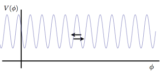
Figure 3: A potential for a scalar field coupled to gravity that could produce bubble distributions of the type we consider.

Even once the potential is symmetric, there are in general nontrivial interactions between bubbles, such as correlations between their nucleation points and collisions between bubbles. We work in the noninteracting limit where the nucleation rate is constant, independent of the presence of other bubbles.

With these assumptions one can compute the bubble distribution on a global time slice. The spacetime is de Sitter with metric

$$ds^{2}={1\over\sin^{2}\eta}\left(-d\eta^{2}+d\Omega_{d}^{2}\right)\ .$$ (2.1)

where $d\Omega_{d}^{2}$ is the metric on a $d$-sphere. The number of bubbles that nucleate in a conformal time interval $d\eta$ is proportional to the spacetime volume available,

$$dN=\gamma dV_{d+1}=\gamma{d\eta\over\sin^{d+1}\eta}d\Omega_{d}$$ (2.2)

where $dV_{d}$ is the $d-$dimensional spacetime volume element and the $d\Omega_{d}$ factor refers to the location of the nucleation point on the spatial slice.

We want to characterize the distribution of bubbles on future infinity of de Sitter space, which is given by $\eta=0$ in these coordinates. A given bubble nucleation nucleation will affect a ball on future infinity. The domain wall of a bubble asymptotically approaches the future lightcone of the nucleation point. Light rays satisfy

$$d\psi=d\eta$$ (2.3)

where $\psi$ is the angular radius of the lightcone. Therefore, a bubble nucleated at time $\eta$ has angular size $\psi=|\eta|$ on the conformal boundary, as shown in figure 4.

Figure 4: A bubble nucleated at conformal time $\eta$ covers an angular size $\psi=|\eta|$ on future infinity.

The distribution of bubbles on the boundary is then

$$dN=\gamma{d\psi\over\sin^{d+1}\psi}d\Omega_{d}\ .$$ (2.4)

Previous attempts to define a theory on such slices can be found in [9, 13].

As mentioned in the introduction, we can also consider the distribution of bubbles which collide with a given “observation bubble.” In [15] we computed this distribution: the distribution of collision bubbles on the boundary of the future lightcone of a point in 3+1 de Sitter space (i.e., the observation bubble’s wall) after infinite time. The number distribution takes the following simple form:

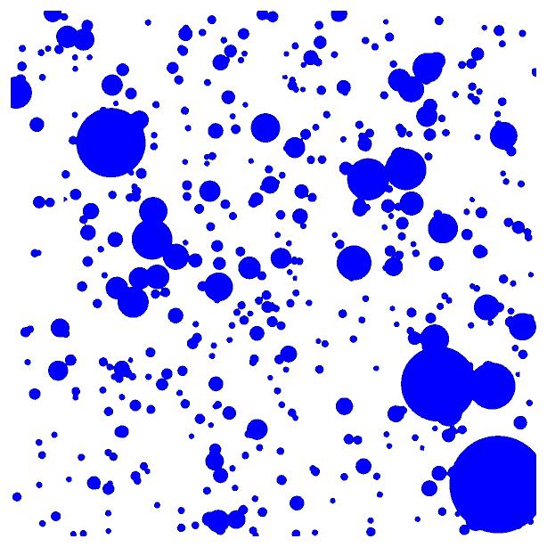
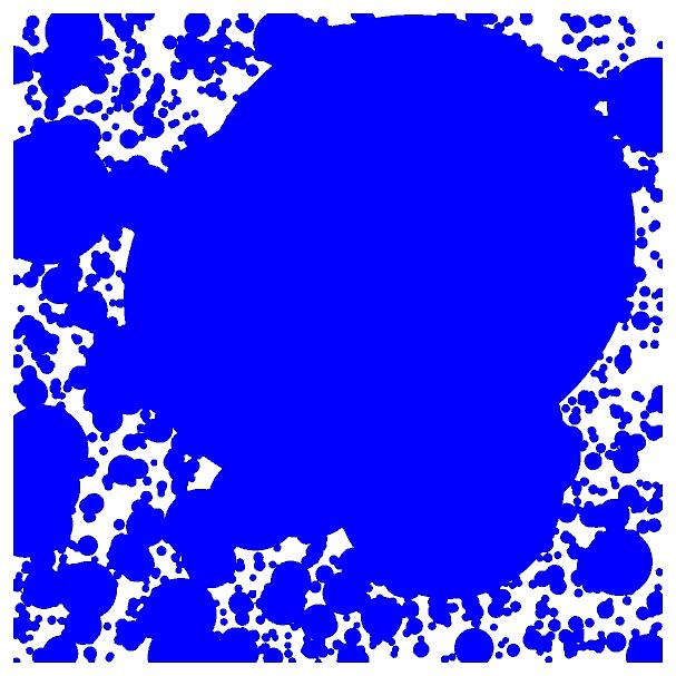
Figure 5: Numerical simulations of the model in $d=2$. Only one disk type is shown. Left pane: $\gamma=.1,\delta/R=.01$. Right pane: $\gamma=.5,\delta/R=.01$.

$$dN(\psi,\theta,\phi)={4\gamma\over 3}{d\psi\over\sin^{3}\psi}\sin\theta d\theta d\phi,$$ (2.5)

where $\psi\in(0,\pi)$ is again the angular radius of the disk, and $\theta$ and $\phi$ are the coordinates of its center on the boundary sphere (we have set the radius of the sphere to 1 for convenience). Notice that this distribution is identical in form to Eq. 2.4 with $d=2$. An attempt to define a conformal field theory on this sphere can be found in [14]. More generally, the number distribution of collisions on the boundary of an “observation bubble” in $d+2$ dimensional de Sitter space is

$$dN=\gamma{\Omega_{d+2}\over\Omega_{d+1}}{d\psi\over\sin^{d+1}\psi}d\Omega_{d}$$ (2.6)

where $\Omega_{n}$ is the surface area of a unit $n$-sphere.

This distribution turns out to have the remarkable property that it is invariant under global conformal transformations $SO(d+1,1)$, which are Mobius transformations in $d=2$. The easiest way to see this is to stereographically project the distribution to the plane. This projection maps spheres to spheres. In terms of the coordinates $x^{i}$ of the center of the sphere and the sphere radius $r$, a little algebra shows that the distribution becomes simply

$$dN=\gamma{dr\over r^{d+1}}{d^{d}x},$$ (2.7)

where $x^{i}$ are the Cartesian coordinates on the plane. Note that this is also the small angular radius, small area approximation to the sphere distribution (2.4). Global conformal transformations on the sphere are generated by rotations plus special conformal transformations. In the stereographic plane, special conformal transformations around the origin take a particularly simple form—they are simply the scalings $x^{i}\rightarrow\lambda x^{i}$ and $r\rightarrow\lambda r$. Therefore the distribution (2.4) is conformally invariant, since it is manifestly rotation invariant, and one can always choose the origin of the stereographic plane to coincide with one of the fixed points of the special conformal transformation. As noted in [15], this symmetry group is the set of Lorentz transformations on the point of nucleation of the observation bubble.

2.1 Fractals and percolation

Benoit Mandelbrot considered the distribution Eq. 2.7 in [16], where he commented that in $d=2$ it approximates the distribution of craters on the moon. One can easily calculate the Minkowski or “box-counting” fractal dimension of various sets of points defined by this distribution. For example, the set of points not inside any bubble is a set of measure zero (because the set of spheres with radii in any given logarithmic interval covers a finite fraction of the volume). To compute the fractal dimension of this set, one chooses boxes of linear dimension $\epsilon$, finds the minimum number $N_{b}(\epsilon)$ of boxes necessary to fully cover the set, and then the dimension is defined as $d_{F}=\lim_{\epsilon\to 0}(-\partial\ln N_{b}/\partial\ln\epsilon)$.

To compute this, note that the volume $V(\epsilon)$ which remains uncovered by spheres of radius greater than $\epsilon$ is the volume $V(\epsilon+d\epsilon)$ minus the volume covered by spheres of size between $\epsilon$ and $\epsilon+d\epsilon$:

$$dV(\epsilon)=-C_{d}\epsilon^{d}dN$$ (2.8)

where $C_{d}$ is the volume of a unit $d$-sphere. The infinitesimal number of spheres is given by

$$dN=\gamma{d\epsilon\over\epsilon^{d+1}}V(\epsilon)\ ,$$ (2.9)

so we have the differential equation

$${dV\over V}=-\gamma C_{d}{d\epsilon\over\epsilon}$$ (2.10)

Integrating this equation gives $V(\epsilon)=V_{0}\epsilon^{\gamma C_{d}}$. The number of cubical boxes of size $\epsilon$ required to cover this area is simply $N_{b}(\epsilon)=V(\epsilon)\epsilon^{-d}$, and therefore [16]

$$d_{F}=d-\gamma C_{d}$$ (2.11)

(see [20] for this calculation in the context of bubbles in $3+1$ de Sitter). Similarly one could compute the dimension of other sets, such as the set of points covered by exactly, or at most, $k$ spheres. These will be scale invariant fractal sets of measure zero as well. The existence of these fractals is not surprising given the statistical scale invariance of the distribution.

One may expect that these sets will undergo percolation transitions at special values of $\gamma$ [16]. For example in $D=2$, as one increases $\gamma$ from zero there should be a percolation critical point where the set transitions from connected along filaments to a disconnected dust. This will occur at some $d_{F}\sim 1$. In $d=3$ one expects two such transitions: from “ramified veils” to filaments at $d_{F}\sim 2$, and from filaments to dust at some other $d_{F}\sim 1$ [16].

If in fact one can regard this as a type of percolation model, it has some novel properties. The most striking is that as we will see, the theory seems to be conformally invariant for all values of $\gamma$ rather than just at the critical points—or at least one can define operators that transform covariantly for all $\gamma$. Additionally, at least some correlation functions can be computed analytically and exactly up to at least the 4-point function. It would be interesting to see if quantities of primary interest for percolation (for example crossing probabilities) could be extracted using the techniques developed here, but we leave this question for future work.

Models of a somewhat similar type have been considered in the past under the name “continuum fractal percolation,” where “continuum” refers to the lack of an underlying lattice, and “fractal” to some self-similarity in the distribution of disks (or other shapes—see e.g. [17]). Another model with some similarities is “Mandelbrot percolation,” in which a square is subdivided into $N^{2}$ smaller squares for some integer $N$, each of which is colored with a probability $p$, and then the remaining uncolored squares are subdivided and the process repeats. Interestingly, while this model does have a percolation transition, it is first order [18]—and hence not conformal even at the transition! Percolation in power-law disk distributions was considered in the context of networks in [19].

3 Correlation functions

In this note we will concentrate on the correlation functions of a field with multiple vacua, as pictured in figure 3. We label the minima by $N$, where $N$ takes integer values. As mentioned earlier, we assume that the vacua are identical, so there is a shift symmetry $N\to N+1$. Starting from a given vacuum, the field can tunnel to the left or to the right; we call these events instantons and anti-instantons.

When the forward lightcones of two spacelike separated nucleation points overlap, additional physics is needed to determine the field profile in the overlap region. If the critical bubble size is small, one can think of these overlap regions as collisions between bubbles. It is then nontrivial and model dependent to solve for what happens in the future of a collision. In our model where the vacua are degenerate, the critical bubble is horizon size, so instead of collisions it is more accurate to think of bubbles nucleating on top of existing domain walls. We make the simplest possible assumption about the overlap regions: we assume the instantons satisfy superposition. In a region to the future of the nucleation points of $N_{+}$ instantons and $N_{-}$ anti-instantons, we assume the field is in the minimum $N=N_{+}-N_{-}$. These simple assumptions allow us to calculate correlation functions explicitly, but it would clearly be interesting to perturb away from them by allowing interactions between nucleation points and nontrivial dynamics in the overlap regions. For small tunneling rate $\gamma$, the instantons are very dilute and one may expect that the interactions are unimportant.

It is convenient to construct a partition function for the bubble distribution with which to compute expectation values. For convenience we will work on the plane, using the distribution (2.7). The partition function is

$$Z=\sum_{n=0}^{\infty}{\gamma^{n}\over n!}\prod_{k=1}^{n}\left(p_{+}+p_{-}\right)^{n}\int_{\delta}^{R}{dr_{k}\over r_{k}^{3}}\int d^{2}x_{k}=\exp{\left(\gamma(p_{+}+p_{-})\int_{\delta}^{R}{dr\over r^{3}}\int d^{2}z\right)}.$$ (3.1)

Each term in the sum corresponds to a configuration of $n$ disks, with the $k$th disk centered at the point $x_{k}$ and with radius $r_{k}$. The factor $(p_{+}+p_{-})$ denotes the probabilities of the two possible types of nucleations, left-moving and right-moving. Because all of the vacua are identical by assumption, detailed balance demands $p_{+}=p_{-}=1/2$. To avoid infinities the integral must be cut off in both small and large disk sizes, although as we will see, well-defined correlation functions on the plane do not depend on the IR cutoff $R$. The factor of $\gamma^{n}$ is the appropriate weight for a configuration of $n$ disks, given that $\gamma\sim e^{-S_{\rm inst}}$ and that instanton interactions can be neglected. The partition function factorizes into instanton and anti-instanton pieces,

$$Z=Z_{+}Z_{-}$$ (3.2)

with

$$Z_{+}=\exp{\left({\gamma_{+}}\int_{\delta}^{R}{dr\over r^{3}}\int d^{2}z\right)}\ .$$ (3.3)

Symmetry determines $\gamma_{+}=\gamma_{-}=\gamma/2$.

Because the distribution is invariant under Mobius transformations, one expects correlation functions of well-defined operators computed using the partition function 3.1 to be Mobius covariant. The subtlety arises from the cutoffs—divergent correlators will not transform simply under Mobius transformations, but as we will see one can define well-behaved operators with correlation functons that transform simply.

The potential has a discrete shift symmetry $N\to N+1$. The natural operators to consider have definite charge under the shift symmetry. The simplest such operators are exponentials,

$$V_{\beta}(z)\equiv e^{i\beta N(z)}\ .$$ (3.4)

We will see that these operators have positive definite weight at least under Mobius transformations, and their correlators are finite in the IR. Correlators of $N$ itself can be determined by differentiating the correlators of exponentials. As we will see this gives logarithms, as one would expect if $N$ were a massless field with dimension zero. Since the correlation functions of such fields are not well-defined, this is another reason to consider exponentials.

3.1 The 1-point function

To compute the 1-point function $\langle V_{\beta}(z)\rangle$ one simply needs to insert it into the partition sum (3.1):

$$\langle V_{\beta}(z)\rangle=Z^{-1}\left(\sum_{n=0}^{\infty}{\gamma_{+}^{n}\over n!}\prod_{k=1}^{n}\int_{\delta}^{R}{dr_{k}\over r_{k}^{3}}\int d^{2}x_{k}e^{i\beta N_{+}(z)}\right)\left(\sum_{n=0}^{\infty}{\gamma_{-}^{n}\over n!}\prod_{k=1}^{n}\int_{\delta}^{R}{dr_{k}\over r_{k}^{3}}\int d^{2}x_{k}e^{-i\beta N_{-}(z))}\right)$$ (3.5)

where the two terms correspond to the instantons and anti-instantons. The exponential operator has a simple product form, and the contributions from the instantons and anti-instantons are complex conjugates of each other, so

$$\langle V_{\beta}(z_{1})\rangle=Z^{-1}\left|\exp\left\{\gamma_{+}\int_{\delta}^{R}{dr\over r^{3}}\int d^{2}x\left[e^{i\beta}\Theta(2r-|x-z_{1}|)+\Theta(-2r+|x-z_{1}|)\right]\right\}\right|^{2}$$ (3.6)

Cancelling against $Z^{-1}$ and collecting terms, this becomes

$$\langle V_{\beta}(z_{1})\rangle=\exp\left[-\gamma(1-\cos\beta)\int_{\delta}^{R}{dr\over r^{3}}\int d^{2}x\Theta(2r-|x-z_{1}|)\right]$$ (3.7)

The integral over $x$ gives the area $A_{1}(r)$ such that a disk of radius $r$ covers $z_{1}$ if its center is contained in $A_{1}$. This set of points is a disk of radius $r$ centered at $z$. Then

$$\langle V_{\beta}(z_{1})\rangle=\exp\left[-\gamma(1-\cos\beta)\int_{\delta}^{R}{dr\over r^{3}}A_{1}(r)\right]$$ (3.8)

The area is $A_{1}=\pi r^{2}$, so the integral is

$$I_{1}\equiv{1\over\pi}\int_{\delta}^{R}{dr\over r^{3}}A_{1}(r)=\ln{R\over\delta}$$ (3.9)

Finally, the one point function of the exponential operator is

$$\langle V_{\beta}(z)\rangle=\left({R\over\delta}\right)^{-\pi\gamma(1-\cos\beta)}=\left\{\begin{array}[]{ c c }1&{\rm if~{}\beta=}2\pi n,~{}n\in{\cal Z}\\ 0&{\rm otherwise}\end{array}\right\}.$$ (3.10)

This type of “conservation of charge” condition is familiar from Liouville theory and free scalar CFTs, but the periodicity in $\beta$ (which is a consequence of the quantization of $N$) is novel.

3.2 The 2-point function

One can compute the 2-point function by the same techniques. A similar analysis to the one above gives

$$\langle V_{\beta_{1}}(z_{1})V_{\beta_{2}}(z_{2})\rangle=\left|\langle\exp\left[i\beta_{1}N(z_{1})+i\beta_{2}N(z_{2})\right]\rangle\right|^{2}=$$ (3.11)

$$\exp{\left\{-\gamma\int{dr\over r^{3}}\int d^{2}x\left(1-\cos\left[\beta_{1}\Theta(r-|x-z_{1}|)+\beta_{2}\Theta(r-|x-z_{2}|)\right]\right)\right\}.}$$ (3.12)

This is equivalent to

$$\langle V_{\beta_{1}}(z_{1})V_{\beta_{2}}(z_{2})\rangle=\exp\left\{-\gamma\int{dr\over r^{3}}\left[(1-\cos\beta_{1})A^{0}_{1}+(1-\cos\beta_{2})A^{0}_{2}+(1-\cos(\beta_{1}+\beta_{2}))A^{0}_{12}\right]\right\}$$ (3.13)

where we have defined the “exclusive area” $A^{0}_{1}$ as the area of the region such that disks centered in that region cover $z_{1}$ but not $z_{2}$. Equivalently, construct two disks of radius $r$, one centered at $z_{1}$ and the other centered at $z_{2}$. Then $A^{0}_{1}$ is the area covered $only$ by the disk centered at $z_{1}$.

Similarly, we define the integral over these areas as

$$I^{0}_{1}(z_{1},z_{2})\equiv{1\over\pi}\int{dr\over r^{3}}A^{0}_{1}(r,z_{1},z_{2})~{}.$$ (3.14)

With this notation, the two point function is

$$\langle V_{\beta_{1}}(z_{1})V_{\beta_{2}}(z_{2})\rangle=\exp\left\{-\pi\gamma\left[(1-\cos\beta_{1})I^{0}_{1}+(1-\cos\beta_{2})I^{0}_{2}+(1-\cos(\beta_{1}+\beta_{2}))I^{0}_{12}\right]\right\}$$ (3.15)

The integrals $I^{0}_{ij...}$ have a simple interpretation as spacetime volumes in de Sitter space: $I^{0}_{ijk}$ is proportional to the spacetime volume available to nucleate bubbles which cover $only$ the points $(z_{i},z_{j},z_{k})$.

To evaluate the integrals, we need to write the exclusive areas in terms of the simpler inclusive areas. For the two-point function, we have

$$A^{0}_{1} = A_{1}-A_{12}$$ (3.16)

$$A^{0}_{2} = A_{2}-A_{12}$$ (3.17)

$$A^{0}_{12} = A_{12}$$ (3.18)

The same equations hold for the integrals of the areas,

$$I^{0}_{1} = I_{1}-I_{12}$$ (3.19)

$$I^{0}_{2} = I_{2}-I_{12}$$ (3.20)

$$I^{0}_{12} = I_{12}$$ (3.21)

We need to compute $I_{12}$, the integral of the area covered by both disks. Some simple geometry yields

$$A_{12}(r,z_{1},z_{2})=2r^{2}\left(\cos^{-1}(|z_{12}|/2r)-(|z_{12}|/2r)\sqrt{1-(|z_{12}|/2r)^{2}}\right)\theta(2r-|z_{12}|),$$ (3.22)

where $|z_{12}|\equiv|z_{1}-z_{2}|$ is the distance between the centers of the disks. Integrating this gives

$$I_{12}(r,z_{1},z_{2})={1\over\pi}\int_{\delta}^{R}A_{12}~{}dr/r^{3}=\ln(R/|z_{12}|)-1/2+{\cal O}(1/R).$$ (3.23)

Plugging this in gives

$$I^{0}_{1}=I^{0}_{2}=\ln{|z_{12}|\over\delta}+{1\over 2}$$ (3.24)

$$I^{0}_{12}=\ln{R\over|z_{12}|}-{1\over 2}$$ (3.25)

Let us redefine the UV cutoff $\delta$ to eliminate the annoying constant factor so that

$$I^{0}_{1}=I^{0}_{2}=\ln{|z_{12}|\over\delta}$$ (3.26)

Note that $I^{0}_{1}$ and $I^{0}_{2}$ are infrared finite, while $I^{0}_{12}$ diverges as $R\to\infty$. This corresponds to an infinite expected number of disks covering both points 1 and 2. Therefore, for $\beta_{1}\neq\beta_{2}$, the exponent of Eq. 3.15 goes to $-\infty$ as the infrared cutoff $R$ is taken to infinity. So the two-point function Eq. 3.11 is zero due to IR divergences. To cancel this divergence it is necessary and sufficient to require that the coefficient of the double overlap region $I^{0}_{12}$ is zero; in other words one needs $\cos(\beta_{1}+\beta_{2})=1$, or $\beta_{1}+\beta_{2}=2\pi n$ ($n$ an integer).

This condition is a kind of charge conservation condition: under the shift symmetry $N\to N+1$, the operator $V_{\beta}$ transforms as $V_{\beta}\to\exp(i\beta)V_{\beta}$. So the correlators are nonzero only when they are invariant under the shift symmetry. Because $N$ takes integer values, the operator $e^{i\beta N(z)}$ is equivalent to the operator $e^{i(\beta+2\pi)N(z)}$, so it is natural that the charge conservation condition is defined mod $2\pi$. We will see in a moment that the dimensions of operators are also periodic functions of $\beta$.

Enforcing this condition we get

$$\langle V_{\beta_{1}}(z_{1})V_{\beta_{2}}(z_{2})\rangle=\left({\delta\over z_{1}-z_{2}}\right)^{\displaystyle\pi\gamma\left(1-\cos\beta_{1}\right)}\left({\delta\over\bar{z}_{1}-\bar{z}_{2}}\right)^{\displaystyle\pi\gamma\left(1-\cos\beta_{1}\right)}$$ (3.27)

when $\beta_{1}+\beta_{2}=2\pi n$ (else the correlator is zero). Defining $\Delta(\beta)=\bar{\Delta}(\beta)={\pi\over 2}\gamma\left(1-\cos\beta\right)$, this has the form of a two-point function for a conformal operator of dimension $(\Delta,\bar{\Delta})$.

3.2.1 Correlation functions of $N$

At this point, we pause for a moment in our analysis of exponential operators to consider quantities which may seem more basic: correlators of the field $N$ itself. Because $N\to-N$ is a symmetry, the 1-point function vanishes, $\langle N(z)\rangle=0$. The 2-point function can be obtained by differentiating the 2-point function of exponentials,

$$\langle N(z_{1})N(z_{2})\rangle=-{\partial\over\partial\beta_{1}}{\partial\over\partial\beta_{2}}\langle V_{\beta_{1}}(z_{1})V_{\beta_{2}}(z_{2})\rangle$$ (3.28)

evaluated at $\beta_{1}=\beta_{2}=0$. A convenient form of the correlator to differentiate is (3.15). Differentiating and setting $\beta_{1}=\beta_{2}=0$ gives

$$\langle N(z_{1})N(z_{2})\rangle=\pi\gamma I^{0}_{12}=\pi\gamma\left(\ln{R\over\left|z_{12}\right|}-{1\over 2}\right)$$ (3.29)

This is the correlation function of a dimension zero field. To put it in a more standard form, the additive factor of $1/2$ could be absorbed into the infrared cutoff and the prefactor $\pi\gamma$ could be absorbed into a field redefinition of $N$. The presence of the infrared divergence means that these correlators are not really well-defined. This is not surprising: since the theory has a symmetry $N\to N+1$, $N$ is not a physical quantity. However, the exponentials we have been considering are physical and have well-defined correlators. Exactly the same issues arise for a free massless scalar in two dimensions.

3.3 The 3-point function

To compute the 3-point function of exponentials $\langle V_{\beta_{1}}(z_{1})V_{\beta_{2}}(z_{2})V_{\beta_{3}}(z_{3})\rangle$ we will need to evaluate the integrals of the overlap regions of three disks of equal size, each centered on a point $z_{i}$ where the operators is inserted. The calculation proceeds along the same lines as for the 2-point function; omitting some details one obtains

$$\langle V_{\beta_{1}}(z_{1})V_{\beta_{2}}(z_{2})V_{\beta_{3}}(z_{3})\rangle=\exp\left\{-\pi\gamma\left[(1-\cos\beta_{1})I^{0}_{1}+(1-\cos\beta_{2})I^{0}_{2}+(1-\cos\beta_{3})I^{0}_{3}\right.\right.+$$

$$(1-\cos(\beta_{1}+\beta_{2}))I^{0}_{12}+(1-\cos(\beta_{1}+\beta_{3}))I^{0}_{13}+(1-\cos(\beta_{2}+\beta_{3}))I^{0}_{23}+\left.\left.(1-\cos(\beta_{1}+\beta_{2}+\beta_{3}))I^{0}_{123}\right]\right\}$$ .

Since the integral $I^{0}_{123}$ is again logarithmically divergent at large $r$, a “charge cancellation” condition is required to cancel the IR divergence that would otherwise send the correlator to zero. Requiring the coefficient of this term be zero means $\beta_{1}+\beta_{2}+\beta_{3}=2\pi n$.

When this condition is satisfied, the correlator simplifies to

$$\langle V_{\beta_{1}}(z_{1})V_{\beta_{2}}(z_{2})V_{\beta_{3}}(z_{3})\rangle=$$

$$\exp\left\{-\pi\gamma\left[(1-\cos\beta_{1})(I^{0}_{1}+I^{0}_{23})+(1-\cos\beta_{2})(I^{0}_{2}+I^{0}_{13})+(1-\cos\beta_{3})(I^{0}_{3}+I^{0}_{12})\right]\right\}$$

The exclusive area integrals are given by, for example,

$$I^{0}_{1} = I_{1}-I_{12}-I_{13}+I_{123}$$ (3.30)

$$I^{0}_{23} = I_{23}-I_{123}$$ (3.31)

The formula for the triple overlap $I_{123}$ is somewhat complicated, but it cancels in the 3-point function, because the integrals appear in combinations such as

$$I^{0}_{1}+I^{0}_{23}=I_{1}-I_{12}-I_{13}+I_{23}$$ (3.32)

Therefore the 3-point function simplifies to

$$\langle V_{\beta_{1}}(z_{1})V_{\beta_{2}}(z_{2})V_{\beta_{3}}(z_{3})\rangle=$$

$$\exp\left\{-\pi\gamma\left[(1-\cos\beta_{1})(I_{1}-I_{12}-I_{13}+I_{23})\right]\right\}\times{\rm(cyclic\ permutations)}$$

In terms of the weights $\Delta_{i}={\pi\over 2}\gamma(1-\cos\beta_{i})$ the 3-point function can be written

$$\langle V_{\beta_{1}}(z_{1})V_{\beta_{2}}(z_{2})V_{\beta_{3}}(z_{3})\rangle=\left|\exp\left\{-(\Delta_{1}+\Delta_{2}-\Delta_{3})(I_{1}-I_{12})\right\}\right|^{2}\times{\rm(cyclic\ permutations)}$$ (3.33)

The combination $(I_{1}-I_{12})$ is exactly the same as in the 2-point function, so

$$\langle V_{\beta_{1}}(z_{1})V_{\beta_{2}}(z_{2})V_{\beta_{3}}(z_{3})\rangle=\left|\left({\delta\over z_{1}-z_{2}}\right)^{\Delta_{1}+\Delta_{2}-\Delta_{3}}\left({\delta\over z_{1}-z_{3}}\right)^{\Delta_{1}+\Delta_{3}-\Delta_{2}}\left({\delta\over z_{2}-z_{3}}\right)^{\Delta_{2}+\Delta_{3}-\Delta_{1}}\right|^{2}$$ (3.34)

This is the 3-point function required by conformal invariance for three operators of weights $\Delta_{i},\bar{\Delta}_{i}$, with $\Delta_{i}=\bar{\Delta}_{i}$. It is worth noting that scale invariance alone is not enough to fix this form—scale invariance requires only that the total scaling dimension of any term on the right-hand side be consistent with the total scaling dimension of the fields in the correlator, but not this particular structure. However global conformal invariance does require this form (in any number of dimensions), because there are no conformal invariants that can be built from less than 4 points.

Starting from the Mobius invariance of the distribution Eq. 2.7 one could presumably prove that well-behaved correlators must be of this form. The statement is non-trivial because of the issue of IR divergences; correlators that depend on the IR regulator will not in general respect this form.

4 Four-point function

In this section we find the 4-point function and analyze its properties. By now the procedure is familiar. The 4-point function is

$$\begin{split}\langle V_{\beta_{1}}(z_{1})V_{\beta_{2}}(z_{2})V_{\beta_{3}}(z_{3})V_{\beta_{4}}(z_{4})\rangle=\exp\{-\pi\gamma[\sum_{i}(1-\cos\beta_{i})I^{0}_{i}+\sum_{i<j}(1-\cos(\beta_{i}+\beta_{j}))I^{0}_{ij}+\\ \sum_{i<j<k}(1-\cos(\beta_{i}+\beta_{j}+\beta_{k}))I^{0}_{ijk}+(1-\cos\sum_{i}\beta_{i})I^{0}_{1234}]\}\end{split}$$ (4.1)

The charge cancellation condition works as before: $I^{0}_{1234}$ is the only infrared divergent quantity, so the correlator is zero unless

$$\sum_{i}\beta_{i}=2\pi n$$ (4.2)

Using the charge cancellation condition, the 4-point function is

$$\begin{split}\langle V_{\beta_{1}}(z_{1})V_{\beta_{2}}(z_{2})V_{\beta_{3}}(z_{3})V_{\beta_{4}}(z_{4})\rangle=\\ \left|\exp\left\{-\Delta_{1}(I^{0}_{1}+I^{0}_{234})-\Delta_{2}(I^{0}_{2}+I^{0}_{341})-\Delta_{3}(I^{0}_{3}+I^{0}_{412})-\Delta_{4}(I^{0}_{4}+I^{0}_{123})-\sum_{i<j}\Delta_{ij}I^{0}_{ij}\right\}\right|^{2}\end{split}$$ (4.3)

where we have defined

$$\Delta_{ij}\equiv{\pi\over 2}\gamma(1-\cos(\beta_{i}+\beta_{j}))$$ (4.4)

Note that due to the charge cancellation condition $\Delta_{12}=\Delta_{34}$.

In the case of four points, the exclusive area integrals are given by

$$I^{0}_{1} = I_{1}-I_{12}-I_{13}-I_{14}+I_{123}+I_{124}+I_{134}-I_{1234}$$ (4.5)

$$I^{0}_{12} = I_{12}-I_{123}-I_{124}+I_{1234}$$ (4.6)

$$I^{0}_{123} = I_{123}-I_{1234}$$ (4.7)

$$I^{0}_{1234} = I_{1234}$$ (4.8)

Using these relations and massaging the expression, the 4-point function can be rewritten

$$\begin{split}&\langle V_{\beta_{1}}(z_{1})V_{\beta_{2}}(z_{2})V_{\beta_{3}}(z_{3})V_{\beta_{4}}(z_{4})\rangle=\\ &\left|\exp\left\{-\sum_{i<j}(\Delta_{i}+\Delta_{j}-\Delta_{ij})(I_{1}-I_{ij})-\left(\sum_{i}\Delta_{i}-{1\over 2}\sum_{i<j}\Delta_{ij}\right)\left(\sum_{i<j<k}I_{ijk}-2I_{1234}-2I_{1}\right)\right\}\right|^{2}\end{split}$$ (4.9)

The first sum has the form of a product over six 2-point functions, while the second term contains a nontrivial function of the positions of the points. To be explicit,

$$\begin{split}&\langle V_{\beta_{1}}(z_{1})V_{\beta_{2}}(z_{2})V_{\beta_{3}}(z_{3})V_{\beta_{4}}(z_{4})\rangle=\\ &\left|\prod_{i<j}\left(\delta\over z_{ij}\right)^{\Delta_{i}+\Delta_{j}-\Delta_{ij}}\exp\left\{-\left(\sum_{i}\Delta_{i}-{1\over 2}\sum_{i<j}\Delta_{ij}\right)\left(\sum_{i<j<k}I_{ijk}-2I_{1234}-2I_{1}\right)\right\}\right|^{2}\end{split}$$ (4.10)

The interesting functional dependence on the location of the points is all contained by the function $f(z_{1},z_{2},z_{3},z_{4})=\sum_{i<j<k}I_{ijk}-2I_{1234}-2I_{1}$.

It is possible to compute the 4-point function in full generality and show that it is conformally invariant. However, since the distribution of bubbles is conformally invariant, the 4-point function is guaranteed to be conformally invariant unless infrared divergences arise. Therefore, we will assume conformal invariance and compute the 4-point function with the four points at

$$z_{1} = z$$ (4.11)

$$z_{2} = 0$$ (4.12)

$$z_{3} = 1$$ (4.13)

$$z_{4} = \infty$$ (4.14)

With this assumption, the four-point function is an infinite constant times a nontrivial function of $z$,

$$\langle V_{\beta_{1}}(z)V_{\beta_{2}}(0)V_{\beta_{3}}(1)V_{\beta_{4}}(\infty)\rangle=C\left|z^{-(\Delta_{1}+\Delta_{2}-\Delta_{12})}(1-z)^{-(\Delta_{1}+\Delta_{3}-\Delta_{13})}\exp\left\{-\left(\sum_{i}\Delta_{i}-{1\over 2}\sum_{i<j}\Delta_{ij}\right)I_{123}\right\}\right|^{2}$$ (4.15)

It now remains to evaluate the integral $I_{123}$.

4.1 Evaluation of the triple overlap integral

We need to evaluate

$$I_{123}\equiv{1\over\pi}\int{dr\over r^{3}}A_{123}$$ (4.16)

where $A_{123}$ is the area contained within the triple overlap of three disks of radius $r$ centered at the points $z_{1},z_{2}$, and $z_{3}$.

To evaluate this we will need a formula for the area of triple overlap of three circles. In some cases this reduces to a double overlap, but in situations where the triple overlap is of triangular type (e.g. a region bounded by the arcs of three distinct circles) the area is [22]:

$$A_{123}={1\over 2}\left(A_{12}+A_{13}+A_{23}-\pi r^{2}\right)+A_{T},$$ (4.17)

where $A_{T}$ is the area of the triangle with vertices at the three points. We will do the computation for triangles for which the triple overlap area is always given by this formula for any disk size $r$, which amounts to assuming that the triangle is sufficiently close to equilateral, with none of the angles exceeding $90^{o}.$ However, our final formula will be valid for any arrangement of three points.

The triple overlap integral begins to be nonzero at the smallest value of $r$ such that a disk can cover all three points. This value is called the circumradius $R_{c}$. By subtracting the area inside a wedge of the circle from a triagular area (see figure 6), we find

$${1\over 2}A_{23}=r^{2}(\pi/2-\theta)-r^{2}\sin\theta\cos\theta$$ (4.18)

where $\theta$ is the angle shown in the figure.

Figure 6: It is convenient to change variables in the integration, using $\theta$ shown in the figure instead of $r$ as the integration variable.

The integral of $A_{23}$ is infrared divergent, but the quantity $A_{23}-\pi r^{2}$ is infrared safe,

$${1\over 2}(A_{23}-\pi r^{2})=-(\theta+\sin\theta\cos\theta)r^{2}$$ (4.19)

so we focus on it. We need to integrate the triple overlap from the lower limit $R_{c}$ where it is first nonzero. So the $A_{23}$ piece of the integral is given by

$${1\over 2}\int_{R_{c}}^{R}{dr\over r^{3}}(A_{23}-\pi r^{2})=-\int_{R_{c}}^{R}{dr\over r}\left[\theta+\sin\theta\cos\theta\right]$$ (4.20)

and we can now freely take $R\to\infty$ because the integral is finite in the infrared. The angle $\theta$ is related to $r$ by

$$\sin\theta={d_{23}\over 2r}$$ (4.21)

Also, as shown in figure 7, the lower limit $r=R_{c}$ corresponds to an upper limit on $\theta$, $\theta=\theta_{1}$, where $\theta_{1}$ is the angle of the triangle with its vertex at point 1. The upper limit $r=\infty$ corresponds to $\theta=0$.

Figure 7: The smallest radius disk which can cover all three points is defined by $r=R_{c}$. The figure shows that the lower limit if integration corresponds to $\theta=\theta_{1}$.

Making the change of variables, the integral is

$${1\over 2}\int_{R_{c}}^{\infty}{dr\over r^{3}}(A_{23}-\pi r^{2})=-\int_{0}^{\theta_{1}}d\theta\left[\theta\cot\theta+\cos^{2}\theta\right]$$ (4.22)

We can now write the full integral.

$$\int_{R_{c}}^{R}{dr\over r^{3}}A_{123}=\int_{R_{c}}^{R}{dr\over r^{3}}\left[{1\over 2}\left((A_{12}-\pi r^{2})+(A_{13}-\pi r^{2})+(A_{23}-\pi r^{2})\right)+\pi r^{2}+A_{T}\right]$$ (4.23)

Now the only infrared divergent term is the trivial $\pi r^{2}$; for the rest of the terms we take $R\to\infty$ to get

$$\int_{R_{c}}^{R}{dr\over r^{3}}A_{123}=\pi\log{R\over R_{c}}+{A_{T}\over 2R_{c}^{2}}-\sum_{i}\int_{0}^{\theta_{i}}(\theta\cot\theta+\cos^{2}\theta)d\theta$$ (4.24)

where the sum is over the three angles of the triangle.

The integral gives

$$\int_{0}^{\theta_{i}}(\theta\cot\theta+\cos^{2}\theta)d\theta=\theta_{i}\ln(\sin\theta_{i})+\theta_{i}({1\over 2}+\ln 2)+{1\over 4}\sin(2\theta_{i})+{1\over 2}\Im\left[{\rm Li_{2}}(e^{2i\theta_{i}})\right]$$ (4.25)

where ${\rm Li_{2}}$ is the dilogarithm function,

$${\rm Li_{2}}(z)\equiv\sum_{n=1}^{\infty}{z^{n}\over n^{2}}$$ (4.26)

We would like to write everything in terms of the angles and lengths of the sides. By examining figure 7, we find

$$2R_{c} = {d_{23}\over\sin{\theta_{1}}}={d_{13}\over\sin{\theta_{2}}}={d_{12}\over\sin{\theta_{3}}}$$ (4.27)

$$A_{T} = R_{c}^{2}\sum_{i}\sin\theta_{i}\cos\theta_{i}$$ (4.28)

We can now rewrite the integral as

$$\begin{split}\pi I_{123}={\pi\over 3}\ln\left({8R^{3}\sin\theta_{1}\sin\theta_{2}\sin\theta_{3}\over d_{12}d_{13}d_{23}}\right)+{1\over 2}\sum_{i}\sin\theta_{i}\cos\theta_{i}\\ -\sum_{i}\left(\theta_{i}\ln(\sin\theta_{i})+\theta_{i}({1\over 2}+\ln 2)+{1\over 4}\sin(2\theta_{i})+{1\over 2}\Im\left[{\rm Li_{2}}(e^{2i\theta_{i}})\right]\right)\end{split}$$ (4.29)

In combining the terms, some simplifications occur because $\sum\theta_{i}=\pi$. A nice symmetric way to write the answer is

$$\pi I_{123}=-{\pi\over 2}+{\pi\over 3}\ln{R^{3}\over\left|z_{12}z_{13}z_{23}\right|}-\sum_{i}\left((\theta_{i}-{\pi\over 3})\ln(\sin\theta_{i})+{1\over 2}\Im\left[{\rm Li_{2}}(e^{2i\theta_{i}})\right]\right)$$ (4.30)

The sum is over all three angles of the triangle formed by the three points, and each angle is defined in the conventional way so that $0\leq\theta_{i}\leq\pi$. Although our derivation is only valid for triangles which are sufficiently close to equilateral, the answer written in this way is valid for any arrangement of the three points.

The answer can also be written in the pleasing form

$$\pi I_{123}=-{\pi\over 2}+\pi\ln R-\theta_{1}\ln d_{23}-\theta_{2}\ln d_{31}-\theta_{3}\ln d_{12}-{1\over 2}\sum_{i}\Im\left[{\rm Li_{2}}(e^{2i\theta_{i}})\right]$$ (4.31)

It is particularly simple when the three points are on a line. If point 2 is between points 1 and 3, then $\theta_{1}=\theta_{3}=0$ and $\theta_{2}=\pi$, so that

$$I_{123}=-1/2+\ln R-\ln d_{31}\ \ \ \ {\rm(collinear)}$$ (4.32)

because all of the dilogarithms vanish.

Having written the answer in terms of the angles, we want to write it as a function of $z$ for our special choice of points,

$$z_{1}=z$$

$$z_{2}=0$$

$$z_{3}=1$$

The angles should satisfy $0\leq\theta_{i}\leq\pi$. For $\Im(z)>0$ we have

$$e^{2i\theta_{1}} = {\bar{z}(1-z)\over z(1-\bar{z})}$$ (4.34)

$$e^{2i\theta_{2}} = {z\over\bar{z}}$$ (4.35)

$$e^{2i\theta_{3}} = {1-\bar{z}\over 1-z}$$ (4.36)

The above is not valid for $\Im(z)<0$, but it is clear that the correct answer should be invariant under $z\to\bar{z}$, so we will just work it out for $z$ in the upper half plane and determine the value in the lower half plane by symmetry.

We rewrite the answer piece by piece in terms of $z$. To write the dilogarithm part of the answer in terms of $z$, it is convenient to rewrite the answer in terms of the Bloch-Wigner function ${\rm D_{2}}$. The relation is

$${\rm D_{2}}(z)=\Im[{\rm Li_{2}}(z)]+\arg(1-z)\ln|z|$$ (4.37)

so that ${\rm D_{2}}(e^{i\theta})=\Im[{\rm Li_{2}}(e^{i\theta})]$. The combination which appears in the answer is

$${1\over 2}\sum_{i}{\rm D_{2}}\left(e^{2i\theta_{i}}\right)={1\over 2}\left\{{\rm D_{2}}\left(z\over\bar{z}\right)+{\rm D_{2}}\left(\bar{z}(1-z)\over z(1-\bar{z})\right)+{\rm D_{2}}\left(1-\bar{z}\over 1-z\right)\right\}={\rm D_{2}}(z)$$ (4.38)

where we have used an identity of the Bloch-Wigner function to get the last equality (see [24] section 7.2).

For the part not involving dilogarithms, we need to solve for $\theta_{i}$ in terms of $z$. Again for $z$ in the upper half plane, we can invert (4.36) to get

$$i\theta_{2} = \ln\left(z\over|z|\right)$$

$$-i\theta_{3} = \ln\left(1-z\over|1-z|\right)$$ (4.39)

subject to the usual convention that the branch cut for the logarithm is taken to be on the negative real axis. $\theta_{1}$ is not needed because in the answer it multiplies $\ln d_{23}$, which is zero. Plugging these in and simplifying,

$$-\theta_{1}\ln d_{23}-\theta_{2}\ln d_{31}-\theta_{3}\ln d_{12}=-\Im\left[\ln z\ln(1-\bar{z})\right]$$ (4.40)

So the answer as a function of $z$ is

$$\pi I_{123}=-{\pi\over 2}+\pi\ln R-\Im[\ln z\ln(1-\bar{z})]-{\rm D_{2}}(z)\ \ \ {\rm for}\ \Im(z)>0$$ (4.41)

Now our algebra has been done under the assumption that $z$ is in the upper half plane, but the answer must be symmetric under $z\to\bar{z}$. The answer as it stands is a constant term plus two functions which are odd under $z\to\bar{z}$. Therefore, the correct answer has an additional factor of the sign of the imaginary part of z,

$$\pi I_{123}=-{\pi\over 2}+\pi\ln R-{\rm sgn}(\Im(z))\left\{\Im[\ln z\ln(1-\bar{z})]+{\rm D_{2}}(z)\right\}$$ (4.42)

4.2 Properties of the 4-point function

Plugging this in, we have the 4-point function

$$\langle V_{\beta_{1}}(z)V_{\beta_{2}}(0)V_{\beta_{3}}(1)V_{\beta_{4}}(\infty)\rangle=C\left|z^{-\Delta_{1}-\Delta_{2}+\Delta_{12}}(1-z)^{-\Delta_{1}-\Delta_{3}+\Delta_{13}}\right|^{2}\times$$

$$\exp\left\{\left({2\over\pi}\sum_{i}\Delta_{i}-{1\over\pi}\sum_{i<j}\Delta_{ij}\right){\rm sgn}(\Im(z))\left\{\Im[\ln z\ln(1-\bar{z})]+{\rm D_{2}}(z)\right\}\right\}$$ (4.43)

By conformal invariance, aside from simple prefactors which depend on the conformal weights of the fields, the 4-point function can depend only on the cross ratio. For our choice of points the cross ratio is just $z$:

$$z={(z_{1}-z_{2})(z_{4}-z_{3})\over(z_{3}-z_{2})(z_{4}-z_{1})}~{}.$$ (4.44)

The 4-point function in a conformal field theory should be crossing-symmetric—it should be invariant under interchanging the points where the operators are inserted. Interchanging the points corresponds to the following group of transformations on $z$:

$$z\to 1-{1\over z}\to{1\over 1-z}\to{1\over z}\to 1-z\to{-z\over 1-z}$$ (4.45)

The last three are odd permutations of the four points; the rest are even [25]. The Bloch-Wigner function ${\rm D_{2}}(z)$ has the property that it changes sign under odd permutations and is invariant under even permutations [25]. Since the sgn function changes sign only under odd permutations, ${\rm sgn}(\Im(z)){\rm D_{2}}(z)$ is invariant under all permutations.

The other nontrivial factor in the 4-point function, (${\rm sgn}(\Im(z))\Im[\ln z\ln(1-z)]$), is slightly more complicated, but one can check that under permutations it transforms in the correct way to contribute the right factors. To take a nontrivial example, under $z\to 1/z$ this function transforms as

$${\rm sgn}(\Im(z^{-1}))\Im[\ln z^{-1}\ln(1-\bar{z}^{-1})]={\rm sgn}(\Im(z))\Im[\ln z\ln(1-\bar{z})]-\pi\ln|z|.$$ (4.46)

One can use this to check that the 4-point function Eq. 4.2 satisfies

$$\langle V_{\beta_{1}}(z)V_{\beta_{2}}(0)V_{\beta_{3}}(1)V_{\beta_{4}}(\infty)\rangle=z^{-2\Delta_{1}}\bar{z}^{-2\Delta_{1}}\langle V_{\beta_{1}}(1/z)V_{\beta_{4}}(0)V_{\beta_{3}}(1)V_{\beta_{2}}(\infty)\rangle,$$ (4.47)

which is the correct behavior [21].

The four-point function simplifies when all 4 points are on a line, or more generally a circle. Using the simple form (4.32) for the triple overlap integral, for $z$ real and negative we have

$$\langle V_{\beta_{1}}(z)V_{\beta_{2}}(0)V_{\beta_{3}}(1)V_{\beta_{4}}(\infty)\rangle=C\left|z^{-\Delta_{1}-\Delta_{2}+\Delta_{12}}(1-z)^{-\Delta_{1}-\Delta_{3}+\Delta_{13}}\right|^{2}\times$$

$$\exp\left\{\left(2\sum_{i}\Delta_{i}-\sum_{i<j}\Delta_{ij}\right)\ln|1-z|\right\}\ \ \ \ (z\ {\rm real\ and\ negative})~{}.$$ (4.48)

Therefore for all 4 points on a circle, the 4-point function is simply a product of power laws; the powers which appear depend on the order of the points.

However, there is a problem. Without the sgn factor, the functions in the exponent in Eq. 4.2 would be odd under $z\to\bar{z}$. Furthermore, they are real analytic functions away from lines of discontinuity running along the real axis from $-\infty$ to $0$ and from $1$ to $+\infty$. So before multiplying by the sign function, the exponent is a real analytic function in a finite region around $z=1/2$. Therefore after including the sign the 4-point function is not real analytic as we drag $z$ across the real axis near $z=1/2$, even though $z$ is separated from the other points at 0 and 1 by a finite distance. In a conventional field theory, correlation functions should be analytic except when two points approach each other.

The nonanalyticity of the 4-point function indicates that the system we have defined does not correspond to a full-fledged conformal field theory. This is not too surprising, because we have made a number of approximations in treating the physics of bubble nucleation; one may still expect that our system can be obtained as the limit of a genuine conformal field theory. We will discuss this further in the conclusions.

5 Central charge

Conformal field theories on curved spaces have a conformal anomaly. Specifically, in 2D CFTs $T^{a}_{~{}a}=-{c\over 12}{\hat{R}}$, where $\hat{R}$ is the scalar curvature of the 2D space. Since the trace of the stress tensor is related to the variation of the action with respect to the conformal factor in the metric, one can compute $c$ by taking the derivative of $\ln Z$ with respect to the log of the curvature. On a sphere of radius $R$,

$$Z(R)=R^{c/3}Z_{0},$$ (5.1)

where $Z_{0}$ is the partition function on a sphere of unit radius [23].

Given the results of the previous section, it is at best unlikely that the theory as we have defined it is a full conformal field theory. Nevertheless we will proceed, as we can easily compute $Z$ on a sphere. The partition function is

$$Z=\sum_{n=1}^{\infty}{\gamma^{n}\over n!}\int d\Omega_{2}\left(\int_{\epsilon}^{\pi-\epsilon}{d\psi\over\sin^{3}\psi}-\Lambda\right),$$ (5.2)

where $\epsilon$ is a cutoff on disk angular size and $\Lambda$ is a (cosmological) constant added as a local counterterm to cancel the leading UV divergence from small $\epsilon$ (as a constant multiplicative factor in $Z$ it cancels out of all the correlators computed earlier). Computing the integral and restoring the dimensions gives

$$\ln Z=4\pi\gamma\left({R^{2}\over\epsilon^{2}}+\ln{R\over\epsilon}+\ln 2-{1\over 6}-\Lambda R^{2}+{\cal O}(\epsilon^{2})\right).$$ (5.3)

Setting the counterterm $\Lambda=1/\epsilon^{2}$ cancels the quadratic UV divergence, but the log is an anomaly that cannot be cancelled with any local counterterm. This is precisely what one expects for a 2D CFT on a sphere with central charge

$$c=12\pi\gamma~{}.$$ (5.4)

For $c<1$, unitarity implies that $c$ must take a discrete set of values (the minimal models). Therefore if this calculation is taken seriously it indicates that our model cannot be unitary at small $\gamma$. However it is worth mentioning that we have included neither perturbative fluctuations of the field nor of the geometry. One expects graviton fluctuations to contribute a term of order $(M_{P}/H)^{d-2}$, and so it is possible that the term we have computed is only one of several contributions to the central charge of a putative complete theory. At large $\gamma$, it is reasonable to expect that the instanton fluctuations are the dominant contribution, and indeed in that limit the theory becomes free. It would be interesting to compare this limit to the analogue in AdS space, where one would take $G_{N}\to 0$ with the AdS radius held fixed so that $c\to\infty$.

5.1 CFT on a fractal

In the string theory landscape there are so-called “terminal vacua”: minima with either zero or negative cosmological constant. A region which tunnels to one of these minima has at most a finite probability of nucleating any more bubbles before infinite time (for a zero CC bubble) or a big crunch (for a negative CC bubble). How best to deal with these regions is unclear, but the proposal of [13] is to excise them and attempt to define a CFT on the remaining space, perhaps including lower dimensional defect CFTs on the boundaries.

A simple toy model for terminal vacua in our 2D CFT is to assume there is some rate $\gamma$ to produce “dead” disks. Following the suggestion of [13] then corresponds to computing correlators in the regions outside these dead disks. Since the region covered by zero disks of any type is a fractal set of measure zero, these correlators will “live” on a fractal set.

One immediate problem is that when $\gamma$ is large this set is not just measure zero, but empty (recall that $d_{F}=d-\gamma\Omega_{d}$, and when $d_{F}\leq 0$ the set is empty). One can consider the case of $\gamma<1$ and continue, but it is clear that the resulting theory will have a very different structure than what we have considered so far.

Since the set is by definition $N(z)=0$ one cannot compute correlators of the disk number operator in the way we have been proceeding. There are two obvious approaches one could take to this. One is to compute the probability that some set of points $z_{i}$ in the full space are all in the set, or various conditional probabilities (such as the odds that if one point is in the set, the others are as well). Computing these probabilities is not difficult using the techniques we have already developed, and the results depend on the distances between the points. However proceeding in this manner we have not succeeded in defining a set of probabilities that are independent of the IR cutoff. The problem in a nutshell is that the number of disks which covers some but not all of a certain set of points is IR finite when integrated against the distribution, but on the other hand the number of disks that would cover all of the points is infrared divergent.

Another approach is to consider more types of disks: a “dead” type which defines the fractal, and then one or more other “live” types. One could then try to compute correlators of the number operator for “live” disks within the set of points covered by zero “dead” disks. However this analysis requires taking into account interactions between the different types of bubbles, something which we will not consider in this note.

6 Generalization to arbitrary dimension

The definition of the theory can be easily generalized to arbitrary dimensions. The partition function in $d$ dimensions is

$$Z=Z_{+}Z_{-}$$ (6.1)

with

$$Z_{+}=\exp\left(\gamma_{+}\int_{\delta}^{R}{dr\over r^{d+1}}\int d^{d}x\right)$$ (6.2)

We will show that the two and three point functions generalize in a simple way. To make the discussion here easier to follow, we include some formulas and discussion which overlap with the earlier sections of the paper.

The general N-point function is

$$\langle e^{i\beta_{1}N(z_{1})}e^{i\beta_{2}N(z_{2})}...e^{i\beta_{n}N(z_{n})}\rangle=\exp(-2C_{d}\gamma[\sum_{i=1}^{n}(1-\cos\beta_{i})I^{0}_{i}+\sum_{i<j}(1-\cos(\beta_{i}+\beta_{j}))I^{0}_{ij}+$$

$$\sum_{i<j<k}(1-\cos(\beta_{i}+\beta_{j}+\beta_{k}))I^{0}_{ijk}+...])$$ (6.3)

where now $z_{i}$ is a point in $d$-dimensional space and $C_{d}$ is the volume of a unit $d$-sphere. As before, define the integral

$$I^{0}_{1}\equiv{1\over C_{d}}\int{dr\over r^{d+1}}A^{0}_{1}(r,z_{i})~{}.$$ (6.4)

The two-point function when the charge conservation condition is satisfied is

$$\langle e^{i\beta N(z_{1})}e^{-i\beta N(z_{2})}\rangle=\exp(-C_{d}\gamma(1-\cos\beta)(I^{0}_{1}+I^{0}_{2}))$$ (6.5)

Now $I^{0}_{1}=I^{0}_{2}=I_{1}-I_{12}$ as before. The 2-point function is then

$$\langle e^{i\beta N_{1}}e^{-i\beta N_{2}}\rangle=\exp(-2C_{d}\gamma(1-\cos\beta)(I_{1}-I_{12}))$$ (6.6)

The integral is given by

$$I_{1}-I_{12}={1\over C_{d}}\int_{\delta}^{R}{dr\over r^{d+1}}A_{1}(r)-{1\over C_{d}}\int_{d_{12}/2}^{R}{dr\over r^{d+1}}A_{12}(r,d_{12})$$ (6.7)

It is helpful to rewrite this as

$$I_{1}-I_{12}={1\over C_{d}}\int_{\delta}^{d_{12}\over 2}{dr\over r^{d+1}}A_{1}(r)-{1\over C_{d}}\int_{d_{12}\over 2}^{R}{dr\over r^{d+1}}\left[A_{1}(r)-A_{12}(r,d_{12})\right]$$ (6.8)

The first term can be integrated immediately using $A_{1}(r)=C_{d}r^{d}$ to get

$$I_{1}-I_{12}=\ln\left(d_{12}\over 2\delta\right)-{1\over C_{d}}\int_{d_{12}\over 2}^{R}{dr\over r^{d+1}}\left[A_{1}(r)-A_{12}(r,d_{12})\right]$$ (6.9)

The remaining integral can be evaluated explicitly, but the crucial information can be extracted more cheaply. The first term, the integral of $A_{1}$, diverges logarithmically at large $r$. However, the second term cancels this divergence, because the double overlap region $A_{12}$ asymptotically has the same area as a single disk,

$$A_{12}\to C_{d}r^{d}\ \ {\rm as}\ r\to\infty~{}.$$ (6.10)

Therefore, the integral is infrared finite, and we can take $R\to\infty$, so that the integral is

$${1\over C_{d}}\int_{d_{12}\over 2}^{\infty}{dr\over r^{d+1}}\left[A_{1}(r)-A_{12}(r,d_{12})\right]$$ (6.11)

This formula depends only on the dimensionful quantity $d_{12}$, but dimensional analysis shows that the answer must be dimensionless. Therefore it is a constant independent of the distance $d_{12}$. So finally

$$I_{1}-I_{12}=\ln\left(d_{12}\over\delta\right)-\#_{d}$$ (6.12)

where $\#_{d}$ is a dimension-dependent constant.

Plugging this in, we have

$$\langle e^{i\beta N(z_{1})}e^{-i\beta N(z_{2})}\rangle=e^{-2C_{d}\gamma(1-\cos\beta)\#_{d}}\left(\delta\over|z_{12}|\right)^{2C_{d}\gamma(1-\cos\beta)}$$ (6.13)

The prefactor can be absorbed into a redefinition of the ultraviolet cutoff $\delta$. The dimension of the vertex operator $e^{i\beta N}$ is

$$\Delta=\bar{\Delta}={C_{d}\over 2}\gamma(1-\cos\beta)$$ (6.14)

Having found the dimensions we can rewrite the general n-point function,

$$\langle e^{i\beta_{1}N(z_{1})}e^{i\beta_{2}N(z_{2})}...e^{i\beta_{n}N(z_{n})}\rangle=\left|\exp\left\{-\sum_{i=1}^{n}\Delta_{i}I^{0}_{i}-\sum_{i<j}\Delta_{ij}I^{0}_{ij}-\sum_{i<j<k}\Delta_{ijk}I^{0}_{ijk}-...\right\}\right|^{2}$$ (6.15)

Now to evaluate the 3-point function explicitly. In general, we have

$$\langle e^{i\beta_{1}N(z_{1})}e^{i\beta_{2}N(z_{2})}e^{i\beta_{3}N(z_{3})}\rangle=\left|\exp\left\{-\Delta_{1}I^{0}_{1}-\Delta_{2}I^{0}_{2}-\Delta_{3}I^{0}_{3}-\Delta_{12}I^{0}_{12}-\Delta_{13}I^{0}_{13}-\Delta_{23}I^{0}_{23}-\Delta_{123}I^{0}_{123}]\right\}\right|^{2}$$ (6.16)

The correlation function is zero unless $\Delta_{123}=0$ because $I^{0}_{123}$ is infrared divergent. $\Delta_{123}=0$ when the charge conservation condition is satisfied, $\beta_{1}+\beta_{2}+\beta_{3}=2\pi n$ with $n$ an integer. Using the charge conservation condition, we have relations like $\Delta_{12}=\Delta_{3}$. Also, recall that the exclusive volumes are given by

$$I^{0}_{1} = I_{1}-I_{12}-I_{13}-I_{23}+I_{123}$$ (6.17)

$$I^{0}_{12} = I_{12}-I_{123}$$ (6.18)

so the 3-point function becomes

$$\left|\exp\left\{-\Delta_{1}(I_{1}-I_{12}-I_{13}+I_{23})-\Delta_{2}(I_{2}-I_{12}-I_{23}+I_{13})-\Delta_{3}(I_{3}-I_{32}-I_{13}+I_{12})])\right\}\right|^{2}$$ (6.19)

Note that the triple overlap region $I_{123}$ does not appear. Collecting terms, we have

$$\left|\exp\left\{-(\Delta_{1}+\Delta_{2}-\Delta_{3})(I_{1}-I_{12})-(\Delta_{1}+\Delta_{3}-\Delta_{2})(I_{1}-I_{13})-(\Delta_{2}+\Delta_{3}-\Delta_{1})(I_{2}-I_{23})\right\}\right|^{2}$$ (6.20)

where we have used $I_{1}=I_{2}=I_{3}$. But this factorizes into 2-point functions! This is precisely the form the 3-point function must take due to conformal invariance. Explicitly, it is

$$\langle e^{i\beta_{1}N(z_{1})}e^{i\beta_{2}N(z_{2})}e^{i\beta_{3}N(z_{3})}\rangle=({\delta^{2}\over z_{12}\bar{z}_{12}})^{\Delta_{1}+\Delta_{2}-\Delta_{3}}({\delta^{2}\over z_{13}\bar{z}_{13}})^{\Delta_{1}+\Delta_{3}-\Delta_{2}})({\delta^{2}\over z_{23}\bar{z}_{23}})^{\Delta_{2}+\Delta_{3}-\Delta_{1}}$$ (6.21)

where we have absorbed the same constant factor into the definition $\delta$ as in the 2-point function.

Now for the 4-point function. Performing a similar analysis as for the 3-point function, we find

$$\langle e^{i\beta_{1}N_{1}}e^{i\beta_{2}N_{2}}e^{i\beta_{3}N_{3}}e^{i\beta_{4}N_{4}}\rangle=\left|\exp\left\{-\sum_{i<j}(\Delta_{i}+\Delta_{j}-\Delta_{ij})(I_{1}-I_{ij})\right\}\right|^{2}\times$$

$$\left|\exp\left\{-C_{\Delta}(I_{123}+I_{124}+I_{134}+I_{234}-2I_{1234}-2I_{1})\right\}\right|^{2}$$ (6.22)

with the definition

$$C_{\Delta}=\Delta_{1}+\Delta_{2}+\Delta_{3}+\Delta_{4}-\Delta_{12}-\Delta_{13}-\Delta_{14}\ .$$ (6.23)

The first factor has the form of factorized two point functions, so we can rewrite this as

$$\langle e^{i\beta_{1}N_{1}}e^{i\beta_{2}N_{2}}e^{i\beta_{3}N_{3}}e^{i\beta_{4}N_{4}}\rangle={\displaystyle\prod_{i<j}}\left(\delta^{2}\over|z_{ij}|^{2}\right)^{\Delta_{i}+\Delta_{j}-\Delta_{ij}}\times$$ (6.24)

$$\left|\exp\left\{-C_{\Delta}(I_{123}+I_{124}+I_{134}+I_{234}-2I_{1234}-2I_{1})\right\}\right|^{2}$$ (6.25)

So the first part of the 4-point function consists of simple power laws. The last line has all of the interesting information in it, and involves the triple and quadruple overlaps. This term is IR finite on its own, but it does depend on the UV cutoff through $I_{1}$; this dependence is trivial.

Computing the 4-point function explicitly is a nontrivial task which we have only accomplished in $d=2$ so far.

6.1 Free field limit

Our correlators have a free-field limit when the tunneling rate becomes large. In taking $\gamma\to\infty$, the expectation value of $N$ will become very large. Operators which are well-defined in this limit should have $\beta_{i}\to 0$. More preciesly, defining

$$\beta=\alpha\sqrt{2\over\pi\gamma}$$ (6.26)

we want to take the limit $\gamma\to\infty$ with $\alpha$ fixed.

To see this that the correlators factorize in this limit, start from the formula for an n-point correlator in general dimension, Eq. 6.15:

$$\langle e^{i\beta_{1}N(z_{1})}e^{i\beta_{2}N(z_{2})}...e^{i\beta_{n}N(z_{n})}\rangle=\left|\exp\left\{-\sum_{i=1}^{n}\Delta_{i}I^{0}_{i}-\sum_{i<j}\Delta_{ij}I^{0}_{ij}-\sum_{i<j<k}\Delta_{ijk}I^{0}_{ijk}-...\right\}\right|^{2}.$$ (6.27)

The exclusive integrated areas $I_{ijk...}^{0}$ satisfy the obvious generalizations of Eqs. 4.5:

$$I_{i_{1}i_{2}...i_{k}}^{0}=\sum_{l=0}^{n-k}{(-1)^{l}\over l!}\sum_{j_{1},j_{2},...,j_{l}}I_{i_{1}i_{2}...i_{k}j_{1}...j_{l}}$$ (6.28)

where the $j$ indices are summed from $1$ to $n$ and the factor of $l!$ corrects for overcounting. In this expression we have defined $I_{ijk...}=0$ if any $i,j,k...$ are equal. Then the exponent in Eq. 6.27 can be written

$$\sum_{k=1}^{n}{\Delta_{i_{1}...i_{k}}\over k!}\sum_{l=0}^{n}{(-1)^{l}\over l!}\sum_{j_{1},j_{2},...,j_{l}}I_{i_{1}i_{2}...i_{k}j_{1}...j_{l}}$$ (6.29)

where we have also defined all areas with $m$ indices $I_{i_{1}i_{2}...i_{m}}=0$ if $m>n$.

To continue, we would like to evaluate the coefficient of the areas $I_{i_{1}i_{2}...i_{l}j_{1}...j_{m-l}}$ with $m$ indices, which is:

$$\sum_{l=0}^{m-1}{(-1)^{l}\over l!(m-l)!}\Delta_{i_{1}...i_{m-l}}\sum_{j_{1},j_{2},...,j_{l}}I_{i_{1}i_{2}...i_{m-l}j_{1}...j_{l}}~{}.$$ (6.30)

In the limit $\beta_{i}\to 0$, we have

$$\Delta_{i_{1}...i_{k}}=\pi\gamma(1-\cos(\beta_{i_{1}}+...+\beta_{i_{k}}))=(\alpha_{i_{1}}+...+\alpha_{i_{k}})^{2}+{\cal O}(\alpha^{4}/\gamma).$$ (6.31)

Since $I_{ijk...}$ is completely symmetric,

$$\Delta_{i_{1}...i_{m-l}}I_{i_{1}i_{2}...i_{m-l}j_{1}...j_{l}}=\left((m-l)\alpha_{i_{1}}^{2}+(m-l)(m-l-1)\alpha_{i_{1}}\alpha_{i_{2}}\right)I_{i_{1}i_{2}...i_{m-l}j_{1}...j_{l}}~{}.$$ (6.32)

Therefore Eq. 6.30 is equal to

$$\sum_{i_{1},...,i_{m}=1}^{n}I_{i_{1}...i_{m}}\sum_{l=0}^{m-1}{(-1)^{l}\over l!}\left({\alpha_{i_{1}}^{2}\over(m-l-1)!}+{\alpha_{i_{1}}\alpha_{i_{2}}\over(m-l-2)!}\right)=\sum_{i_{1},...,i_{m}=1}^{n}I_{i_{1}...i_{m}}\left(\alpha_{I_{1}}^{2}\delta_{m,1}+\alpha_{i_{1}}\alpha_{i_{2}}\delta_{m,2}\right).$$ (6.33)

So only the 1- and 2-disk overlap areas contribute! Therefore the exponent in Eq. 6.27 becomes simply

$$-\alpha_{i}^{2}I_{i}-\alpha_{i}\alpha_{j}I_{ij}.$$ (6.34)

Recalling that $I_{i}=\ln(R/\delta)$ and $I_{ij}=\ln(R/|z_{ij}|)(1-\delta_{ij})$, and using $\sum_{i}\alpha_{i}^{2}=\sum_{ij}\left(\alpha_{i}\alpha_{j}-\alpha_{i}\alpha_{j}(1-\delta_{ij})\right)$, we get

$$\langle e^{i\beta_{1}N(z_{1})}e^{i\beta_{2}N(z_{2})}...e^{i\beta_{n}N(z_{n})}\rangle=\left|\exp\left\{-\sum_{i,j}\alpha_{i}\alpha_{j}\left(\ln{R\over\delta}+\ln{\delta\over|z_{ij}|}(1-\delta_{ij})\right)\right\}\right|^{2}.$$ (6.35)

As usual this is IR divergent unless we impose conservation of charge, which here is simply $\sum_{i}\alpha_{i}=\sum_{i,j}\alpha_{i}\alpha_{j}=0$. Then, recalling that $\beta N(z)=\sqrt{2}\alpha\phi(z)$

$$\langle e^{i\sqrt{2}\alpha_{1}\phi(z_{1})}e^{i\sqrt{2}\alpha_{2}\phi(z_{2})}...e^{i\sqrt{2}\alpha_{n}\phi(z_{n})}\rangle=\prod_{i<j}\left|{z_{i}-z_{j}\over\delta}\right|^{4\alpha_{i}\alpha_{j}}.$$ (6.36)

This is the general form of a correlation function of vertex operators $e^{i\sqrt{2}\alpha\phi(z)}$ of a free massless field in $D=2$ (see e.g. [21], p. 296). In higher dimensions a non-interacting massless scalar with non-canonical kinetic term $\phi\Box^{d/2}\phi$ could produce such correlators.

7 Conclusions

Starting from eternal de Sitter space we have successfully defined a model with correlation functions that are conformally covariant and transform with positive weight. However because of the lack of analyticity in the 4-point function, the model does not appear to be a healthy conformal field theory (except perhaps in the non-interacting $\gamma\to\infty$ limit).

One possibility is that the theory we have defined here is the limit of some good CFT in which certain effects have been ignored. Such limits can result in non-analyticities in correlation functions (for example, one can get logs from power laws by expanding around a limit where the dimensions of some operators go to zero). Adding weight to this possibility is that in defining the simplest possible non-trivial model, we indeed have ignored many potentially important effects:

• We have ignored perturbative fluctuations of the field around its minima, and included only the instantons.

• We have ignored perturbative corrections to the instantons themselves, which for example include fluctuations away from spherical shape.

• We have ignored interactions between the instantons other than their collisions, and we have treated collisions and overlaps in a simplistic manner.

• We have used a semi-classical approximation that ignores quantum interference between different configurations in the ensemble of bubbles.

• We have ignored gravitational fluctuations in the bulk, as well as fluctuations in the geometry of the boundary.

• The bulk theory we considered is a single scalar field in de Sitter space. Even coupled to gravity, such a model in anti-de Sitter space probably does not define a consistent CFT—one presumably needs the infinite number of modes of string theory, or at least one expects some very restrictive conditions on the bulk degrees of freedom necessary to define a good dual. Perhaps similar restrictions apply here.

From this point of view the model described here is only a potentially interesting first step on the path to a full theory of inflation or de Sitter space. Nevertheless, we feel the basic structure may be correct, and indeed many of the effects mentioned above could be included as perturbations around our limit. In addition, the model may have interested applications to condensed matter systems or as an example of a new class of conformally invariant theories. We hope to investigate some of these issues further in the future.

References

- [1] R. Bousso and J. Polchinski, “Quantization of four-form fluxes and dynamical neutralization of the cosmological constant,” JHEP 0006, 006 (2000) [arXiv:hep-th/0004134].
- [2] L. Susskind, “The anthropic landscape of string theory,” arXiv:hep-th/0302219.
- [3] S. R. Coleman and F. De Luccia, “Gravitational Effects On And Of Vacuum Decay,” Phys. Rev. D 21, 3305 (1980).
- [4] B. Freivogel, M. Kleban, M. Rodriguez Martinez and L. Susskind, “Observational consequences of a landscape,” JHEP 0603, 039 (2006) [arXiv:hep-th/0505232].
- [5] S. Chang, M. Kleban and T. S. Levi, “Watching Worlds Collide: Effects on the CMB from Cosmological Bubble Collisions,” arXiv:0810.5128 [hep-th].
- [6] E. Witten, “Quantum gravity in de Sitter space,” arXiv:hep-th/0106109.
- [7] L. Dyson, J. Lindesay and L. Susskind, “Is there really a de Sitter/CFT duality,” JHEP 0208, 045 (2002) [arXiv:hep-th/0202163].
- [8] L. Dyson, M. Kleban and L. Susskind, “Disturbing Implications of a Cosmological Constant,” JHEP 0210, 011 (2002) [arXiv:hep-th/0208013].
- [9] A. Strominger, “The dS/CFT correspondence,” JHEP 0110, 034 (2001) [arXiv:hep-th/0106113].
- [10] N. Goheer, M. Kleban and L. Susskind, “The trouble with de Sitter space,” JHEP 0307, 056 (2003) [arXiv:hep-th/0212209].
- [11] A. H. Guth, “Eternal inflation and its implications,” J. Phys. A 40, 6811 (2007) [arXiv:hep-th/0702178].
- [12] L. Susskind, “The Census Taker’s Hat,” arXiv:0710.1129 [hep-th].
- [13] J. Garriga and A. Vilenkin, “Holographic Multiverse,” JCAP 0901, 021 (2009) [arXiv:0809.4257 [hep-th]].
- [14] B. Freivogel, Y. Sekino, L. Susskind and C. P. Yeh, “A holographic framework for eternal inflation,” Phys. Rev. D 74, 086003 (2006) [arXiv:hep-th/0606204].
- [15] B. Freivogel, M. Kleban, A. Nicolis and K. Sigurdson, “Eternal Inflation, Bubble Collisions, and the Disintegration of the Persistence of Memory,” arXiv:0901.0007 [hep-th].
- [16] B. B. Mandelbrot, The Fractal Geometry of Nature (W. H. Freeman, 1982).
- [17] R. Meester and R. Roy, Continuum Percolation (Cambridge University Press, 1996).
- [18] J. Chayes, L. Chayes, and R. Durrett, “Connectivity properties of Mandelbrot’s percolation process,” Probab. Theory Related Fields 77 (1988), no. 3.
- [19] C. Warren, L. Sander, and I. Sokolov, “Geography in a scale-free network model,” Phys. Rev. E 66 (2002).
- [20] A. Vilenkin, “Did the universe have a beginning?,” Phys. Rev. D 46, 2355 (1992).
- [21] P. Di Francesco, P. Mathieu, D. Senechal, Conformal Field Theory, Springer (1999).
- [22] K. Kratky, “The area of intersection of n equal circular disks,” J. Phys. A: Math. Gen. 11 1017 (1978).
- [23] A. Zamolodchikov, “Scaling Lee-Yang model on a sphere. I: Partition function,” JHEP 0207, 029 (2002) [arXiv:hep-th/0109078].
- [24] G.A. Ray, “Multivariable Polylogarithm Identities,” in Structural Properties of Polylogarithms, Ed. L. Lewin, American Mathematical Society, 1991.
- [25] D. Zagier, “The Dilogarithm Function,” in Frontiers in Number Theory, Physics, and Geometry II, Springer Berlin Heidelberg, 2007