Experimental investigation of Wigner’s reaction matrix for irregular graphs with absorption

Abstract

We use tetrahedral microwave networks consisting of coaxial cables and attenuators connected by $T$-joints to make an experimental study of Wigner’s reaction $K$ matrix for irregular graphs in the presence of absorption. From measurements of the scattering matrix $S$ for each realization of the microwave network we obtain distributions of the imaginary and real parts of $K$. Our experimental results are in good agreement with theoretical predictions.

Pauling introduced quantum graphs of connected one-dimensional wires almost seven decades ago Pauling . Kuhn used the same idea a decade later Kuhn to describe organic molecules by free electron models. Quantum graphs can be considered as idealizations of physical networks in the limit where the lengths of the wires greatly exceed their widths; this corresponds to assuming that propagating waves remain in a single transverse mode. Among the systems modeled by quantum graphs are, e.g., electromagnetic optical waveguides Flesia ; Mitra , mesoscopic systems Imry ; Kowal , quantum wires Ivchenko ; Sanchez and excitation of fractons in fractal structures Avishai ; Nakayama . Recent work has shown that quantum graphs provide an excellent system for studies of quantum chaos Kottossmilansky ; Kottos ; Prlkottos ; Zyczkowski ; Kus ; Tanner ; Kottosphyse ; Kottosphysa ; Gaspard ; Blumel ; Hul2004 . Quantum graphs with external leads (antennas) have been analyzed in detail in Kottosphyse ; Kottosphysa . Quantum graphs with absorption, a more realistic but more complicated system, have been studied numerically in Hul2004 , but until now there have been no experimental studies of the effect of absorption.

This paper presents results of our experimental study of distributions of Wigner’s reaction matrix Akguc2001 (often called in the literature just the $K$ matrix Fyodorov2004 ) for microwave networks that correspond to graphs with time reversal symmetry ($\beta=1$ symmetry class of random matrix theory Mehta ) in the presence of absorption. For the case of an experiment having a single-channel antenna, the $K$ matrix and scattering matrix $S$ are related by

$$S=\frac{1-iK}{1+iK}.$$ (1)

The function $Z=iK$ has direct physical meaning as the electrical impedance, which has been recently measured in a microwave cavity experiment Anlage2005 . For the one-channel case the $S$ matrix can be parameterized as

$$S=\sqrt{R}e^{i\theta},$$ (2)

where $R$ is the reflection coefficient and $\theta$ is the phase.

After seminal work of López, Mello and Seligman Lopez1981 came theoretical studies of the properties of statistical distributions of the $S$ matrix with direct processes and imperfect coupling Doron1992 ; Brouwer1995 ; Savin2001 . A recent experiment investigated the distribution of the $S$ matrix for chaotic microwave cavities with absorption Kuhl2005 . The distribution $P(R)$ of the reflection coefficient $R$ in Eq. (2), at the beginning investigated in the strong absorption limit Kogan , has been recently known for any dimensionless absorption strength $\gamma=2\pi\Gamma/\Delta$, where $\Gamma$ is the absorption width and $\Delta$ is the mean level spacing. For systems with time reversal symmetry ($\beta=1$) Méndez-Sánchez et al.  Sanchez2003 studied $P(R)$ experimentally, and Savin et al.  Savin2005 found an exact formula for $P(R)$. For systems violating time reversal symmetry ($\beta=2$), Beenakker and Brouwer Beenakker2001 calculated $P(R)$ for the case of a perfectly coupled, single-channel lead.

In our experiment we simulate quantum graphs with microwave networks. The analogy between them is based on the Schrödinger equation for the former being equivalent to the telegraph equation for the latter Hul2004 . We call them microwave graphs. Measurements of the scattering matrix for them were stimulated by Blumel88 and the pioneering measurements in Doron90 .

A simple microwave graph, the tetrahedral case, consists of six coaxial cables (bonds) that meet three-at-a-time at $N=4$ different $T$-joints (vertices). Each coaxial cable consists of an inner conductor with radius $r_{1}$ separated from a concentric outer conductor with inner radius $r_{2}$ by a homogeneous, non-magnetic material with dielectric constant $\varepsilon$. The fundamental $TEM$ mode that propagates (the so-called Lecher wave) down to zero frequency exists because the cross section of the cable is doubly connected (Jones, , p. 253). For frequencies $\nu$ below the onset of the TE₁₁ mode in a coaxial cable, which propagates above $\nu_{c}\simeq\frac{c}{\pi(r_{1}+r_{2})\sqrt{\varepsilon}}$ Jones , the cable is single mode: only the TEM mode propagates. For SMA-RG-402 coaxial cable, which has $r_{1}=0.05$ cm, $r_{2}=0.15$ cm, and $\varepsilon\simeq 2.08$ (teflon dielectric), single-mode propagation occurs below 32.9 GHz.

An (ideal) microwave graph with no aborption and no leads to the outside world is a closed (bound) system. The presence of absorption and/or leads to the outside world creates an open system. Because the coaxial cables are lossy, we may vary absorption in the microwave graphs by changing the length of cable(s), Hul2004 , by adding one or more (coaxial) microwave attenuators, or by changing the coupling to the outside world.

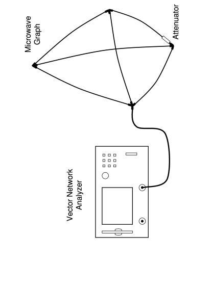
Figure 1: A diagram of experimental setup used to measure the scattering matrix $S$ of tetrahedral microwave graphs with absorption. Absorption in the graphs was varied by changing the attenuator. The vector network analyzer used for all measurements was an HP model 8722D.

Figure 1 shows our experimental setup for measurements of the single-channel scattering matrix $S$ for tetrahedral microwave graphs. We used a Hewlett-Packard model 8722D microwave vector network analyzer to measure the scattering matrix $S$ of such graphs in two different frequency windows, viz., 3.5–7.5 GHz and 12-16 GHz. As the figure shows, at one of the four vertices we used a 4-joint connector to couple the microwave graph to the vector network analyzer via a single-channel lead realized with an HP model 85133-60017, low-loss, flexible microwave cable; the other three vertices consisted of $T$-joints. The plane of calibration in the measurements was at the entrance to the 4-joint connector. Note that the microwave graph in Fig. 1 has a microwave attenuator in one of its bonds.

To investigate the distributions of imaginary and real parts of the $K$ matrix we measured the scattering matrix $S$ for $184$ different realizations of tetrahedral microwave graphs having a microwave (SMA) attenuator in one of the bonds. For each graph realization, which was obtained either by the replacement of the bonds or putting an attenuator to a different bond, the scattering matrix $S$ was measured in 1601 equally spaced steps. The total optical lengths of the microwave graphs, including joints and the single attenuator, was 196.2 cm when a 3 dB, 6 dB, or 20 dB attenuator was used, whereas it was 197.4 cm when the 10 dB attenuator was used. To avoid degeneracy of eigenvalues in the graphs, we chose optical lengths for the bonds that were not simply commensurable.

Figure 2: Panels (a) and (b) show, respectively, the modulus $|S|$ and the phase $\theta$ of the scattering matrix $S$ measured for the graph (see Fig. 1) with absorption parameter $\gamma=3.6$ (see the text) over the frequency range 12 - 13.4 GHz and with use of a 3 dB attenuator. Panels (c) and (d) show corresponding measurements for a graph with $\gamma=6.8$ over the same frequency range and with use of a 20 dB attenuator. The total optical length, 196.2 cm, of both microwave graphs was the same, including joints and the attenuator.

Figure 2 shows the modulus $|S|$ and the phase $\theta$ of the scattering matrix $S$ of a tetrahedral graph with $\gamma=3.6$ (in panels (a) and (b), obtained with use of a 3 dB attenuator) and one with $\gamma=6.8$ (in panels (c) and (d), obtained with use of a 20 dB attenuator); both cases cover the frequency range 12–13.4 GHz. The lengths of corresponding bonds in the two graphs were the same. Direct processes are present in the scattering because the microwave vector analyzer was connected to the graphs by the 4-joint connector. For each, individual realization of the graph we may estimate them from the average value of the scattering matrix $\langle S\rangle$. Our measurements averaged over all realizations of microwave graphs gave $\langle S\rangle_{av}\simeq 0.47\pm 0.03+i(-0.01\pm 0.04)$, where $i=\sqrt{-1}$. The experimental value for $|\langle S\rangle_{av}|\simeq 0.47$ is close to a theoretical estimate Kottosphyse ; Kottosphysa for the modulus of the vertex reflection amplitude $|\rho|=0.5$ for a 4-joint connector with Neumann boundary conditions,

$$\rho=\frac{2}{n_{v}}-1,$$ (3)

where $n_{v}=4$ is the number of bonds meeting at the vertex in question.

Equation (1) holds for systems with absorption but without direct processes. The case of imperfect coupling $|\langle S\rangle|>0$ and direct processes present can be mapped onto that of perfect one Fyodorov2004 by making the following parametrization,

$$S_{0}=\frac{S-|\langle S\rangle|}{1-|\langle S\rangle|S},$$ (4)

where $S_{0}$ is the scattering matrix of a graph for the perfect-coupling case (no direct processes present).

For systems with time reversal symmetry ($\beta=1$ in equations below), the distributions $P(v)$ of the imaginary and $P(u)$ of the real parts of the $K$ matrix Fyodorov2004 are given by the following interpolation formulas:

$$P(v)=\frac{N_{\beta}e^{-a}}{\pi\sqrt{2\gamma}v^{3/2}}(A[K_{0}(a)+K_{1}(a)]a+\sqrt{\pi}Be^{-a}),$$ (5)

and

$$P(u)=\frac{N_{\beta}e^{-\gamma/4}}{2\pi\bar{u}}[\frac{A}{2}\sqrt{\frac{\gamma}{4}}D(\frac{\bar{u}}{2})+BK_{1}(\frac{\gamma\bar{u}}{4})],$$ (6)

where $-v=\textrm{Im}\,K<0$ and $u=\textrm{Re}\,K$ are, respectively, the imaginary and real parts of the $K$ matrix. The normalization constant is $N_{\beta}=\alpha\left(A\Gamma(\beta/2+1,\alpha)+Be^{-\alpha}\right)^{-1}$, where $\alpha=\gamma\beta/2$, $\Gamma(x,\alpha)=\int_{\alpha}^{\infty}dtt^{x-1}e^{-t}$ is the upper incomplete Gamma function, $A=e^{\alpha}-1$ and $B=1+\alpha-e^{\alpha}$. In Eq. (5) the variable $a=\frac{\gamma}{16}(\sqrt{v}+1/\sqrt{v})^{2}$ and $K_{0}$, $K_{1}$ are MacDonald functions. In Eq. (6) $D(z)=\int_{0}^{\infty}dq\sqrt{1+z(q+q^{-1})}e^{-\gamma z(q+q^{-1})/4}$ and $\bar{u}=\sqrt{u^{2}+1}$.

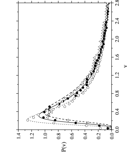
Figure 3: Experimental distribution $P(v)$ of the imaginary part of the $K$ matrix at different values of the mean absorption parameter: $\bar{\gamma}=3.8$ (open circles), $\bar{\gamma}=5.2$ (full circles) and $\bar{\gamma}=6.7$ (open triangles), respectively. Each corresponding theoretical distribution $P(v)$ evaluated from Eq. (5) is also shown: $\gamma=3.8$ (dotted line), $\gamma=5.2$ (solid line), and $\gamma=6.7$ (dashed line), respectively.

Figure 3 shows experimental distributions $P(v)$ for three mean values of the parameter $\bar{\gamma}$, viz., 3.8, 5.2, and 6.7. The distribution for $\bar{\gamma}=3.8$ is obtained by averaging over 69 realizations of microwave graphs having $\gamma$ within the window $[3.5,\,4.1]$. The distribution for $\bar{\gamma}=5.2$ is obtained by averaging over 60 realizations of microwave graphs having $\gamma$ within the window $[4.7,\,5.6]$. The distribution for $\bar{\gamma}=6.7$ is obtained by averaging over 55 realizations of microwave graphs having $\gamma$ within the window $[6.3,\,7.1]$. We estimated the experimental values of the $\gamma$ parameter by adjusting the theoretical mean reflection coefficient $\langle R\rangle_{th}$ to the experimental one $\langle R_{0}\rangle=\langle S_{0}S_{0}^{{\dagger}}\rangle$, where

$$\langle R\rangle_{th}=\int_{0}^{1}dRRP(R).$$ (7)

We also applied the following interpolation formula Kuhl2005 for the distribution $P(R)$:

$$P(R)=N_{\beta}\frac{e^{-\frac{\alpha}{1-R}}}{(1-R)^{2+\beta/2}}[A\alpha^{\beta/2}+B(1-R)^{\beta/2}].$$ (8)

We offer the following comment on the validity of the Eq. (8). We used it instead of exact formulas (12-14) recently presented in Savin2005 , which may be used to find the distribution $P(R)$, because Eq. (8) is sufficiently accurate (see Fig. 1 in Savin2005 ) while allowing for much faster numerical calculations.

Figure 3 also presents for comparison with each experimental distribution $P(v)$ (symbols) the corresponding numerical distribution (lines) evaluated from Eq. (5). We see that the experimental distribution $P(v)$ at $\bar{\gamma}=3.8$ and at 5.2 agree well with their theoretical counterparts. However, the comparison for $\bar{\gamma}=6.7$ shows some discrepancies, particularly in the range $0.3<v<0.8$.

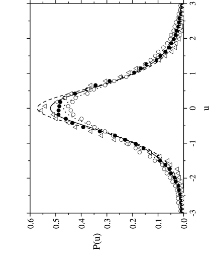
Figure 4: Experimental distribution $P(u)$ of the real part of the $K$ matrix at different values of the mean absorption parameter: $\bar{\gamma}=3.8$ (open circles), $\bar{\gamma}=5.2$ (full circles) and $\bar{\gamma}=6.7$ (open triangles), respectively. Each corresponding theoretical distribution $P(u)$ evaluated from Eq. (6) is also shown: $\gamma=3.8$ (dotted line), $\gamma=5.2$ (solid line), and $\gamma=6.7$ (dashed line), respectively.

We may use measurements of the distribution $P(u)$ of the real part of Wigner’s reaction matrix for an imporant and natural consistency check on our determination of $\gamma$. Figure 4 compares experimental and theoretical $P(u)$ distributions at the aforementioned values of $\bar{\gamma}$, viz., 3.8, 5.2, and 6.7. Though each case shows good overall agreement between experimental and theoretical results, for all three cases the middle ($-0.25<u<0.25$) of the theoretical distribution is slightly higher than its experimental counterpart. According to the definition of the $K$ matrix (see Eq. (1)), such behavior of the experimental distribution $P(u)$ suggests a deficit of small values of $|\textrm{Im}\,S_{0}|$. We do not yet know the origin of this deficit.

Though there are the small discrepancies we have mentioned, the good overall agreement between experimental and theoretical results justifies a posteriori the procedure we have used to determine the experimental values of $\gamma$.

The distributions $P(v)$ and $P(u)$ of imaginary and real parts of Wigner’s reaction matrix may be also found using the alternative approach described in Anlage2005 ; Anlage2005b . In these papers the radiation impedance approach was developed and used to obtaining the distributions of real and imaginary parts of the normalized impedance

$$Z=\frac{\textrm{Re }Z_{c}+i(\textrm{Im }Z_{c}-\textrm{Im }Z_{r})}{\textrm{Re }Z_{r}}$$ (9)

of a chaotic microwave cavity, where $Z_{c(r)}=Z_{0}(1+S_{c(r)})/(1-S_{c(r)})$ is the cavity (radiation) impedance expressed by the cavity (radiation) scattering matrix $S_{c(r)}$ and $Z_{0}$ is the characteristic impedance of the transmission line. The radiation impedance $Z_{r}$ is the impedance seen at the input of the coupling structure for the same coupling geometry, but with the sidewalls removed to infinity. This interesting approach is especially useful in the studies of microwave systems, in which, in general, both the system and radiation impedances are measurable. However, it is not obvious how to use in practice this approach in the case of quantum systems.

We used this alternative approach to find distributions $P(v)$ and $P(u)$ of imaginary and real parts of Wigner’s reaction matrix for irregular tetrahedral microwave graphs. Wigner’s reaction matrix can be simply expressed by the normalized impedance $K=-iZ$. The radiation impedance $Z_{r}$ was found experimentally by measuring in two different frequency windows, viz., 3.5–7.5 GHz and 12-16 GHz of the scattering matrix $S_{r}$ of the 4-joint connector with three joints terminated by 50 $\Omega$ terminators.

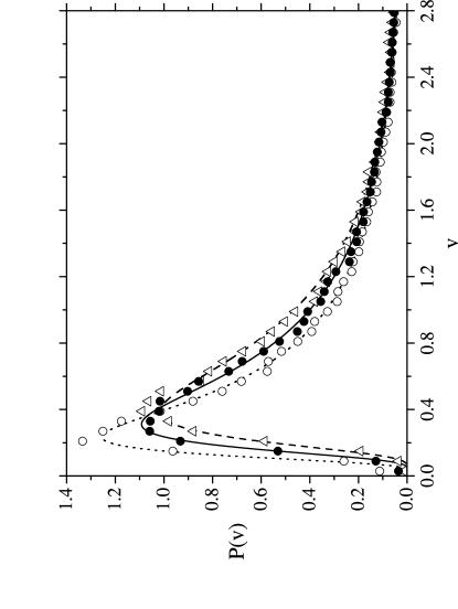
Figure 5: Experimental distribution $P(v)$ of the imaginary part of the $K$ matrix at different values of the mean absorption parameter: $\bar{\gamma}=3.8$ (open circles), $\bar{\gamma}=5.2$ (full circles) and $\bar{\gamma}=6.7$ (open triangles), respectively, calculated using the radiation impedance approach Anlage2005 ; Anlage2005b . Each corresponding theoretical distribution $P(v)$ evaluated from Eq. (5) is also shown: $\gamma=3.8$ (dotted line), $\gamma=5.2$ (solid line), and $\gamma=6.7$ (dashed line), respectively.

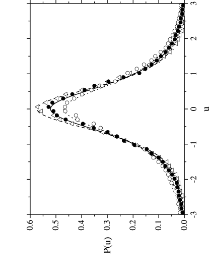
Figure 6: Experimental distribution $P(u)$ of the real part of the $K$ matrix at different values of the mean absorption parameter: $\bar{\gamma}=3.8$ (open circles), $\bar{\gamma}=5.2$ (full circles) and $\bar{\gamma}=6.7$ (open triangles), respectively, calculated using the radiation impedance approach Anlage2005 ; Anlage2005b . Each corresponding theoretical distribution $P(u)$ evaluated from Eq. (6) is also shown: $\gamma=3.8$ (dotted line), $\gamma=5.2$ (solid line), and $\gamma=6.7$ (dashed line), respectively.

In Fig. 5 and Fig. 6 we show the distributions $P(v)$ and $P(u)$ calculated using the radiation impedance approach Anlage2005 ; Anlage2005b . As in the case of the scattering matrix approach, the experimental distributions are obtained at three values of the parameter $\bar{\gamma}=3.8$, 5.2 and 6.7. Figure 5 shows that the distribution $P(v)$ of the imaginary part of Wigner’s reaction matrix for $\bar{\gamma}=5.2$ is in good agreement with the theoretical prediction Fyodorov2004 . However, for $\bar{\gamma}=3.8$ and 6.7 the theoretical results are slightly higher than the experimental ones, what is especially noticeable at the peaks of the distributions. The experimental distribution $P(u)$ of the real part of Wigner’s reaction matrix presented in Figure 6 at three values of the parameter $\bar{\gamma}=3.8$, 5.2 and 6.7 displays a very good agreement with the theoretical result. The comparison of Figures 3 and 5 and Figures 4 and 6 show that the distributions $P(v)$ and $P(u)$ evaluated by means of the radiation impedance approach are at the peaks slightly higher than the ones obtained by the scattering matrix approach, what may suggest that the influence of the phase of $S_{r}$ on the distributions is not negligible Anlage2005b .

In summary, using the scattering matrix approach and the radiation impedance approach we have measured distributions $P(v)$ and $P(u)$ of imaginary and real parts of Wigner’s reaction matrix for irregular tetrahedral microwave graphs consisting of SMA cables, connectors, and attenuators. Use of different attenuators allowed us to vary absorption in the graphs in a controlled, quantitative way. For the case of time reversal symmetry ($\beta=1$), the experimental results for $P(v)$ and $P(u)$ calculated for both approaches at the same three values of the mean parameter $\bar{\gamma}$ are in good overall agreement with theoretical predictions.

Acknowledgments: This work was supported by KBN grant No. 2 P03B 047 24 and an equipment grant from ONR(DURIP).

References

- (1) L. Pauling, J. Chem. Phys. 4, 673 (1936).
- (2) H. Kuhn, Helv. Chim. Acta, 31, 1441 (1948).
- (3) C. Flesia, R. Johnston, and H. Kunz, Europhys. Lett. 3 , 497 (1987).
- (4) R. Mitra and S. W. Lee, Analytical techniques in the Theory of Guided Waves (Macmillan, New York, 1971).
- (5) Y. Imry, Introduction to Mesoscopic Systems (Oxford, New York, 1996).
- (6) D. Kowal, U. Sivan, O. Entin-Wohlman, Y. Imry, Phys. Rev. B 42, 9009 (1990).
- (7) E. L. Ivchenko, A. A. Kiselev, JETP Lett. 67, 43 (1998).
- (8) J.A. Sanchez-Gil, V. Freilikher, I. Yurkevich, and A. A. Maradudin, Phys. Rev. Lett. 80 , 948 (1998).
- (9) Y. Avishai and J.M. Luck, Phys. Rev. B 45, 1074 (1992).
- (10) T. Nakayama, K. Yakubo, and R. L. Orbach, Rev. Mod. Phys. 66, 381 (1994).
- (11) T. Kottos and U. Smilansky, Phys. Rev. Lett. 79, 4794 (1997).
- (12) T. Kottos and U. Smilansky, Annals of Physics 274, 76 (1999).
- (13) T. Kottos and U. Smilansky, Phys. Rev. Lett. 85, 968 (2000).
- (14) T. Kottos and H. Schanz, Physica E 9, 523 (2003).
- (15) T. Kottos and U. Smilansky, J. Phys. A 36, 3501 (2003).
- (16) F. Barra and P. Gaspard, Journal of Statistical Physics 101, 283 (2000).
- (17) G. Tanner, J. Phys. A 33, 3567 (2000).
- (18) P. Pakoński, K. Życzkowski and M. Kuś, J. Phys. A 34, 9303 (2001).
- (19) P. Pakoński, G. Tanner and K. Życzkowski, J. Stat. Phys. 111, 1331 (2003).
- (20) R. Blümel, Yu Dabaghian, and R.V. Jensen, Phys. Rev. Lett. 88, 044101 (2002).
- (21) O. Hul, S. Bauch, P. Pakoński, N. Savytskyy, K. Życzkowski, and L. Sirko, Phys. Rev. E 69, 056205 (2004).
- (22) G. Akguc and L. E. Reichl, Phys. Rev. E 64, 056221 (2001).
- (23) Y.V. Fyodorov and D.V. Savin, JETP Letters 80, 725 (2004).
- (24) M.L. Mehta, Random Matrices, (Academic Press, New York, 1991).
- (25) S. Hemmady, X. Zheng, E. Ott, T.M. Antonsen, and S.M. Anlage, Phys. Rev. Lett. 94, 014102 (2005).
- (26) S. Hemmady, X. Zheng, T.M. Antonsen, E. Ott, and S.M. Anlage, Phys. Rev. E 71, 056215 (2005).
- (27) G. López, P.A. Mello, and T.H. Seligman, Z. Phys. A 302, 351 (1981).
- (28) E. Doron and U. Smilansky, Nucl. Phys. A 545, 455 (1992).
- (29) P.W. Brouwer, Phys. Rev. B 51, 16878 (1995).
- (30) D.V. Savin, Y.V. Fyodorov, and H.-J. Sommers, Phys. Rev. E 63, 035202 (2001).
- (31) U. Kuhl, M. Martinez-Mares, R.A. Méndez-Sánchez, and H.-J. Stöckmann, Phys. Rev. Lett. 94, 144101 (2005).
- (32) E. Kogan, P.A. Mello, H. Liqun, Phys. Rev. E 61, R17 (2000).
- (33) R.A. Méndez-Sánchez, U. Kuhl, M. Barth, C.V. Lewenkopf, and H.-J. Stöckmann, Phys. Rev. Lett. 91, 174102-1 (2003).
- (34) D.V. Savin, H.-J. Sommers, and Y.V. Fyodorov, arXiv:cond-mat/0502359 v1, 15 Feb 2005.
- (35) C.W.J. Beenakker and P.W. Brouwer, Physica E 9, 463 (2001).
- (36) D. S. Jones, Theory of Electromagnetism (Pergamon Press, Oxford, 1964), p. 254.
- (37) E. Doron, U. Smilansky, and A. Frenkel, Phys. Rev. Lett. 65, 3072 (1990).
- (38) R. Blümel and U. Smilansky, Phys. Rev. Lett. 60, 477 (1988).