Abstract

We present a brief overview of the regularizing transformations of the Kepler problem and we relate the Euler transformation with the symplectic structure of the phase space of the $N$-body problem. We show that any particular solution of the $N$-body problem where two bodies have rectilinear dynamics can be regularized by a linear symplectic transformation and the inclusion of the Euler transformation into the group of symplectic local diffeomorphisms over the phase space. As an application we regularize a particular configuration of the restricted circular $N$+2 body problem.

Introduction

In Celestial Mechanics, the $N$-body problem has two types of singularities: collisions between two or more bodies, and escapes in bounded time. In order to study the behavior of the system close to singularities, it is a common procedure to transform it to another equivalent system that avoids the singularities by means of some methods called regularizations. There are a lot of regularizing transformations, but unfortunately it is not always possible to regularize an arbitrary singularity. For instance, infinite expansions at finite time produce esential singularities in the mathematical model that are not regularizable by topological or analytical methods known until now, and the same is true for some multiple collisions.

Basically there exist two types of regularizations: analytic regularization formalized by Siegel and Moser [24], regularization by surgery or topological (also known as block regularization) discovered by Conley and Easton [6, 7]. In particular, it is well-known that collisions between two infinitesimal bodies (in $N$+$\nu$ problems) and triple collisions are impossible to regularize by the Easton method [19]. Marchal [19] has a very clear exposition about the classification of the singularities in the $N$-body problem and their regularization (when it is possible).

In this paper we deal with the analytical or Siegel’s regularization [24] which is achieved by three ingredients: a local change of coordinates by means of some local diffeomorphism $\rho:M\to M$ on the phase space, a scaling function $g:M\to\mathbb{R}$ that introduce a new fictitious time $\tau$ by the relation $\frac{dt}{d\tau}=g(w)$ and a set of initial conditions $\phi_{0}=\phi(0)$ of the flow which specifies the solutions that go to collision; since $N$-body problems are Hamiltonian problems, the set of initial conditions determines an energy level by the conservation of the energy. It means that in Hamiltonian problems the analytical regularization process is performed on each fixed energy level $H(x)=h$.

Thus, the process is as follows:

• choose a fixed energy level $H(x)=h$ and consider

  $$(H-h)(x)=0,$$

• apply the change of coordinates $x=\rho(w)$ of the phase space

  $$[(H-h)\circ\rho](w)=0$$

• apply the scaling transformation $\frac{dt}{d\tau}=g(w)$ multiplying the last expression

  $$\Gamma=[g\cdot(H-h)\circ\rho](w)$$

• the preimage of $\Gamma(w,h)=0$ generates the energy levels of the regularized system for each $h\in{\rm Img}(H)\subset\mathbb{R}$ fixed.

It is important to keep in mind that the aim of regularization theory is to transform singular differential equations into regular ones, controlling the velocity of the regularized system by the scaling time [5].

For the one-dimensional Kepler motion with Hamiltonian function

$$H(q,p)=\frac{1}{2}y^{2}-\frac{\mu}{x},\qquad x\in\mathbb{R}^{*},\quad y\in T_{x}\mathbb{R},$$ (1)

it was already found by Euler that the introduction of a square-root coordinate $u=\sqrt{x}$ and a fictitious time $\tau$ defined by $dt=xd\tau$ reduces the Kepler equation of motion (1) to the equation of motion of a one-dimensional harmonic oscillator

$$\mu=\frac{1}{2}v^{2}+h\ u^{2},\qquad u\in\mathbb{R}^{*},\quad v\in T_{u}\mathbb{R},$$ (2)

if $h<0$ [3]; where $y=\frac{dx}{dt}$, $v=\frac{du}{d\tau}$ and $\mathbb{R}^{*}=(\mathbb{R}-\{0\})$.

Generalizing this approach, Levi-Civita introduces its “…transformation du système qui donne lieu à des conséquences remarquables…” in [17, 1907]. In his work Levi-Civita introduces a conformal transformation and exploits the symplectic structure of the complex plane $(\mathbb{C},dz\wedge d\bar{z})\cong(\mathbb{R}^{2},dy\wedge dx)$. In fact, this regularization is made on the cotangent bundle $T^{*}(\mathbb{C}^{*})$ where $\mathbb{C}^{*}=\{z\in\mathbb{C}:z\neq 0\}$ is viewed as an open symplectic manifold. Levi-Civita regularization is achieved by the local diffeomorphism

$$\left.\begin{array}[]{rcl}\rho:(T^{*}(\mathbb{C}^{*}),\omega)&\to&(T^{*}(\mathbb{C}^{*}),\omega)\\ (z,w)&\mapsto&\left(z^{2},\frac{w}{2|z|}\right)\end{array}\right.$$ (5)

and the time rescaling $dt=|z|^{2}d\tau$. The transformation above takes the Hamiltonian function

$$H(q,p)=\frac{1}{2}p^{2}-\frac{\mu}{|q|},\qquad q\in\mathbb{C}^{*},\quad p\in T_{q}\mathbb{C},$$ (6)

into the equation

$$\mu=\frac{1}{2}w^{2}+h|z|^{2},\qquad z\in\mathbb{C}^{*},\quad w\in T_{z}\mathbb{C},$$ (7)

where $p=\frac{dq}{dt}$, $w=\frac{dz}{d\tau}$ and the symplectic form in the regularized phase space is $\omega=d\bar{w}\wedge dz$. The expression (5) is a contact transformation since it preserves the canonical Liouville 1-form $\alpha=\bar{w}dz$. If we denote the image of the local diffeomorphism by $(q,p)=\rho(z,w)$ then

$$\bar{p}dq = \bar{w}dz,$$ (8)

that is, $\rho^{*}(\alpha)=\alpha$; as a consequence we have a symplectic (canonical) transformation. Applying the exterior differential to both sides of (8) we obtain the symplecticity condition $\rho^{*}(\omega)=\omega$ for the transformation. In 1913 Sundman introduced a transformation that maps the unitary circle in $\mathbb{R}^{2}$ into the band $-1<y<1$, and obviously this mapping does not preserves the area [9, pp 127-129].

Unfortunately, the procedure described above is difficult to generalize to the 3-dimensional case since the euclidean space $\mathbb{R}^{3}$ does not posses any complex structure. However, the Kustaanheimo-Stiefel’s regularization [15], generalizes the Levi-Civita regularization to the four dimensional complex manifold $T^{*}\mathbb{C}^{2}$ (real dimension 8) and projects it onto some symplectic submanifold of real dimension 6 [25]. In recent years, the K-S transformation using quaternions and the quaternionic algebra has gained much attention, from the works of Vivarelli [27], Volk [28], Vrbik [29], Waldvogel [30, 31], among others

On the other hand, some of the most recent works for computing collision orbits using symplectic integrators are based on the algorithmic regularization. This procedure was introduced by Mikkola and Tanikawa [21, 22] simultaneously with Preto and Tremaine [23] in 1999. Algorithmic regularization uses a particular time scaling function

$$\frac{dt}{d\tau}=g(w,t),\quad(w,t)\in T^{*}\mathcal{Q}\times\mathbb{R},$$

defined on the extended phase space, instead of the classical $g(q)=f(q)\prod_{i,j}r_{ij}$, where $q\in\mathcal{Q}$ and $r_{ij}=\sqrt{q_{i}-q_{j}}$. The more interesting property of algorithmic regularizations is the absence of a coordinate transformation.

In order to construct the time scaling function $g(w,t)$, the extended phase space $T^{*}\mathcal{Q}\times\mathbb{R}$ is considered as a presymplectic manifold and then immersed into a symplectic one, locally diffeomorphic to $(\hat{M},\omega_{\hat{M}})$ where $\hat{M}=(T^{*}\mathcal{Q}\times T^{*}\mathbb{R})$ and $\omega_{\hat{M}}=\omega-dt\wedge dH$. Then, we search for a function $g:\hat{M}\to\mathbb{R}$ such that the resulting Hamiltonian function $\Lambda=g(z)(H(q,p,t)-h)$ will be separable.

At this point, there exists two types of algorithmic regularization: the logarithmic Hamiltonian and the Time Transformed Leapfrog (TTL). The former is a canonical extension of the original Hamiltonian system to the extended symplectic manifold $(\hat{M},\omega_{\hat{M}})$. The Hamiltonian function $H(q,p)=T(p)-V(q)$ extends to the function

$$\Lambda(Q,P)=\log\left(T_{e}(P)\right)-\log(V(Q))\quad$$

where $P=(p,h)$, $Q=(q,t)$, $T_{e}(P)=T(p)-h$ and $H=h$ is a fixed value. The new independent variable is $\tau=\int_{0}^{t}T(p)-h\ ds$ and the Hamiltonian vector field $X_{\Lambda}$ becomes $\dot{z}=J\nabla_{z}\Lambda(z)$, $z=(Q,P)$.

TTL is a non-canonical generalization of the logarithmic Hamiltonian. In this case, the scaling function $g$ contains the term $\Omega=\sum_{i<j}(\Omega_{ij}/r_{ij})$ for some selected coefficients $\Omega_{ij}\in\mathbb{R}$. The vector field

$$\dot{q}=A^{-1}p,\qquad\dot{p}=F(q)$$

is transformed into

$$q^{\prime}=A^{-1}p/W,\qquad t^{\prime}=1/W,\qquad p^{\prime}=F(q)/W,\qquad W^{\prime}=\frac{\partial\Omega}{\partial q}p.$$

and regularization of two body collisions is obtained if $\Omega\sim 1/r$ near collisions. These “regularizations” have shown a satisfactory behavior in numerical computations close to collisions. However, their geometrical analysis will be considered by the authors in a future work.

1 Symplectic Structure of Regularizing Transformations

In symplectic geometry, mechanical problems are represented by Hamiltonian systems $(M,\omega,X_{H})$ on the phase space viewed as a symplectic manifold. The standard symplectic manifold is the cotangent bundle $M=T^{*}\mathcal{Q}$ of the configuration space $\mathcal{Q}=(\mathbb{R}^{N\cdot n}-\Delta)$, where $\Delta$ is the set of the singularities of $X_{H}$ and $H$. This manifold is provided with the canonical symplectic form $\omega=d{\bf p}\wedge d{\bf q}$ where ${\bf q}\in\mathcal{Q}$ and ${\bf p}\in T^{*}_{\bf q}\mathcal{Q}$.

In particular, problems on celestial mechanics are based on the Newtonian $N$-body equations, $\mathcal{M}\ddot{\bf q}=-\frac{\partial V}{\partial{\bf q}}$ where

$$V({\bf q})=G\sum_{i,j}^{N}\frac{m_{i}m_{j}}{|q_{i}-q_{j}|},\quad{\bf q}=(q_{1},\dots,q_{N}),\quad q_{i}\in\mathbb{R}^{n},\quad 1\leq i\leq N,$$ (9)

$q_{i}$ is the position of the $i$-th body, $m_{i}$ its mass and $\mathcal{M}={\rm diag}(m_{1}I_{n},\dots,m_{N}I_{n})$. Depending on the value of $n$, we refer to this problem as the rectilinear or collinear problem if $n=1$, the planar problem if $n=2$ and the spatial problem if $n=3$. In its Hamiltonian formulation the Hamiltonian function $H:M\to\mathbb{R}$ is defined by

$$H({\bf q},{\bf p})=T({\bf p})-V({\bf q})$$ (10)

where $T({\bf p})={\bf p}^{T}\mathcal{M}^{-1}{\bf p}$ is the kinetic energy.

It is clear that the set of singularities comes from the potential function $V({\bf q})$. As we have said, it is not always possible to regularize any arbitrary singularity, however in this paper we are concerned with sigularities due to binary rectilinear collisions as the generalization of the rectilinear Kepler problem. To avoid this type of singularities we perform a regularizing transformation using a local diffeomorphism $f:M\to M$ and a time rescaling $g:M\to\mathbb{R}$. In some specific cases when it is desirable to preserve the fibers and sections of the cotangent bundle, the diffeomorphism and the time rescaling are applied to the base space $f:\mathcal{Q}\to\mathcal{Q}$ and $g:\mathcal{Q}\to\mathbb{R}$. To obtain a local symplectic diffeomorphism on $M=T^{*}\mathcal{Q}$ one uses the properties of the cotangent lift of $f$.

Definition 1.1

Let $\mathcal{Q}$ be an arbitrary differentiable manifold with cotangent bundle $M=T^{*}\mathcal{Q}$, and let $f\in{\rm Diff}_{x}(\mathcal{Q})$ be any local diffeomorphism over $\mathcal{Q}$, we define the cotangent lift of $f$ by

$$F:=T^{*}f:M\to M;\hskip 30.0ptF(p_{1})=p_{2},$$ (11)

where $p_{i}=(x_{i},\xi_{i})\in M$, $i=1,2$ and $x_{i}\in\mathcal{Q}$, $\xi_{i}\in T^{*}_{x_{i}}\mathcal{Q}$, and $(df_{x_{1}})^{*}\xi_{2}=\xi_{1}$,

Adittionaly we can see that

$$(df_{x_{1}})^{*}:T^{*}_{x_{2}}\mathcal{Q}\to T^{*}_{x_{1}}\mathcal{Q},$$

so the restriction of $F|_{T^{*}_{x_{1}}}$ is the inverse mapping of $(df_{x_{1}})^{*}$.

Proposition 1.1

The cotangent lift $F$ of any local diffeomorphism $f\in{\rm Diff}_{x}(\mathcal{Q})$ is a local symplectomorphism, which means that

$$F^{*}\omega=\omega.$$

where $\omega$ is the canonical symplectic form on $M$.

The standard references where the reader can check the proof are [2, pp 487] and [1, pp 180]. It is easy to show that the mapping

$$T^{*}:{\rm Diff}_{x}(\mathcal{Q}) \to {\rm Sp}_{(x,\xi)}(M,\omega)$$

$$\qquad\qquad f \mapsto F:=T^{*}f.$$

is a homomorphism of groups. (Hereafter all concerned diffeomorphisms are local diffeomorphisms.)

In this way, it is possible to construct symplectomorphisms that preserve the structure of the cotangent bundle in the sense that they are fiberwise transformations. They form a subgroup of ${\rm Sp}(M)$ closely related to the set of generating functions on $M$.

For $N$-body problems in the plane it is a common procedure to identify the real plane with the complex numbers $\mathbb{R}^{2}\cong\mathbb{C}$. Szebehely [26] has noted that in order to have a suitable regularizing transformation for binary collisions in the restricted plane 3-body problem, the conditions

$$z=f(w)\qquad{\rm and}\qquad\frac{dt}{d\tau}=|f_{w}(w)|^{2},$$ (12)

must hold, where $f:\mathbb{C}\to\mathbb{C}$ is a meromorphic function of the complex variable $w=u+iv$.

The expression (12) is a fiberwise transformation which preserves the cotangent bundle as consequence of the cotangent lift of $f:\mathbb{C}\to\mathbb{C}$ to $T^{*}\mathbb{C}$. In such a case, the bilinear form $\omega_{\mathbb{C}}=d\bar{p_{z}}\wedge dz$ gives the symplectic stucture to $T^{*}\mathbb{C}$. Moreover, any fiberwise symplectic regularization of binary collisions in the $N$ center problem has the form equivalent to (12) [14]. This condition can be generalized for symplectic regularizations in higher dimensional spaces as it is exposed in [10] .

As we have said, it was known by Euler that the transformation $u=\sqrt{x}$ and the time rescaling $dt=xd\tau$ reduces the one-dimensional Kepler problem to the one-dimensional harmonic oscillator for $h<0$. This transformation can be rewritten as $x=u^{2}/2$ with time rescaling $dt=u^{2}d\tau$ and it fulfills condition (12) when we restrict $x>0$ and $f:\mathbb{R}^{*}\to\mathbb{R}$.

In order to simplify calculations and preserve the symplectic structure we plug in the coefficient $1/2$ to the transformation and considering the cotangent lift we obtain

$$x=\frac{u^{2}}{2},\qquad y=\frac{v}{u},\qquad dt=u^{2}d\tau.$$ (13)

where $y=\frac{dx}{dt}$ and $v=\frac{du}{d\tau}$. In what follows, we rename the variables $x=q$, $u=Q$, $y=p$ and $v=P$ to agree with the standard notation of Hamiltonian mechanics.

Definition 1.2

Let $\mathcal{N}=\{x\in\mathbb{R}:x>0\}$ be the positive open ray and let $\mathcal{V}=T^{*}\mathcal{N}$ be its cotangent bundle. We define de Euler transformation $\xi:\mathcal{V}\to\mathcal{V}$ as the mapping

$$\xi:(Q,P)\mapsto\left(\frac{Q^{2}}{2},\frac{P}{Q}\right)$$ (14)

where $Q\in\mathcal{V}$ and $P\in T^{*}_{Q}\mathcal{V}$.

We restrict the domain of the Euler transformation to be an open manifold with boundary, in order to consider this transformation as a local diffemorphism.

Lemma 1.2

The Euler transformation $\xi:\mathcal{V}\to\mathcal{V}$ defined in (14) is a (local) symplectomorphism.

Proof. We obtain the result in a straightforward way since the Jacobian matrix

$$(d\xi)=\left(\begin{array}[]{cc}Q&-\frac{P}{Q^{2}}\\ 0&\frac{1}{Q}\end{array}\right)$$ (17)

is symplectic. $\hfill\square$

Definition 1.3

We call Euler regularization of the collinear Kepler problem to the Euler transformation together with the rescaling function $dt=Q^{2}d\tau$ applied to the equation of movement of the Kepler problem.

It is possible to consider the inclusion of the Euler transformation into the group ${\rm Diff}_{x}(M)$ of local diffeomorphisms of any symplectic manifold $(M,\omega)$ containning a two-dimensional linear symplectic subspace $\mathcal{V}$ such that $M\cong\mathcal{V}\oplus\mathcal{V}^{\omega}$.

We recall that a subspace $V\subset E$ of some symplectic vector space $(E,\omega)$ of dimension $2n$, is called symplectic if the restriction of the symplectic form $\omega|_{V}$ is injective (non degenerate).

A well-known result about symplectic vector spaces that will be useful to understand the regularizing transformation applied to the circular $N$+2 Sitnikov problem is the following.

Lemma 1.3

Let $(E,\omega)$ be a symplectic vector space and let $V\subset E$ be a linear subspace. Then $V$ is a symplectic subspace if and only if

$$E=V\oplus V^{\omega}$$ (18)

where $V^{\omega}$ is the orthogonal subspace to $V$ with respect to the bilinear form $\omega$. Moreover, $V^{\omega}$ is a symplectic subspace.

The proof of this result is found in any book on symplectic geometry. Now, we procede to construct the regularizing transformation that we will apply to some symmetric $N$+2 body problems in the simpler cases: regularization of binary rectilinear collisions of the infinitesimals.

Definition 1.4

The canonical inclusion of the Euler transformation into the group ${\rm Diff}_{x}(M)$ of an open symplectic manifold with boundary $(M,\omega)$ is the local diffeomorphism

$$i_{\xi}:\mathcal{V}\oplus\mathcal{V}^{\omega}\to M,$$ (19)

such that

$$i_{\xi}|_{\mathcal{V}}=\xi\qquad and\qquad i_{\xi}|_{\mathcal{V}^{\omega}}=id_{\mathcal{V}^{\omega}}.$$ (20)

We have the relation $\imath\circ\xi=i_{\xi}\circ\imath$, therefore the following diagram comutes

where $\imath(T^{*}\mathcal{N})\cong\mathcal{V}$ is as in Definition 1.3.

Lemma 1.4

The canonical inclusion is a local symplectomorphism $i_{\xi}\in{\rm Sp}_{(x,\xi)}(U,\omega)$ for $U\subset M$ any open subset.

Proof. This fact is obtained straightforward from de direct sum $\mathcal{V}\oplus\mathcal{V}^{\omega}$, then the Jacobian matrix of the differential is

$$d(i_{\xi})=\left(\begin{array}[]{c|c}(d\xi)&0\\ \hline\cr 0&I_{2(n-1)}\end{array}\right),$$ (24)

where $d\xi\in\mathcal{M}_{2\times 2}$ is the Jacobian matrix of the Euler transformation and $I_{2(n-1)}$ is the identity matrix in $\mathcal{M}_{2(n-1)\times 2(n-1)}$. $\square$

2 Some symmetric N+2 body problems

Now, we must to characterize particular solutions of the $N$ body problem where the Euler regularization is applied in a natural way. Since Euler regularization only considers the unidimensional (rectilinear) evolution of the colliding bodies we focus our attention to systems with $N$ massive and 2 infinitesimal bodies and we call them $N+2$ body problems.

Definition 2.1

We say that a solution $\varphi(t)=\varphi(\varphi_{0},t)$ of the spatial $N$ body problem has an $\mathscr{R}$-symmetry around the line $\mathcal{L}\subset\mathbb{R}^{3}$ if $\mathscr{R}\in SO(3)$ satisfies the following properties:

• for every $t\in(\alpha,\beta)$ and every state $S=((q_{i}(t),p_{i}(t)),\cdots,(q_{N}(t),p_{N}(t)))$ the action of $\mathscr{R}$ on $S$ is a cyclic permutation of order $r>1$,

• for every $x\in\mathcal{L}$ we have $\mathscr{R}x=x$.

It is clear that the $\mathscr{R}$-symmetry applies to the whole phase space since this is valid in the configuration space for every $t\in(\alpha,\beta)$. This is equivalent to a selection of $\mathscr{R}$-symmetric initial condition $\varphi(0)=\varphi_{0}$ in the phase space $M=T^{*}(\mathbb{R}^{3N}-\Delta)$ and follow the flow $\Phi^{t}(\varphi_{0})$.

Remark 2.1

It is possible to have the limits $\alpha=-\infty$ or $\beta=\infty$ however, in the general case, the $\mathscr{R}$-symmetry is valid for solutions which comes or goes to singularities when $t^{+}\to\alpha$ or $t^{-}\to\beta$.

Proposition 2.1

Let $\varphi(t)$ be an $\mathscr{R}$-symmetric solution of the spatial $N$ body problem for $t\in(\alpha,\beta)$, around the fixed line $\mathcal{L}\subset\mathbb{R}^{3}$ and we consider the restricted $N+1$ body problem attaching an infinitesimal body to the $\mathscr{R}$-symmetric solution. If the restricted body has initial conditions

$$\left(\begin{array}[]{c}q_{I}(t_{0})\\ p_{I}(t_{0})\end{array}\right)=\left(\begin{array}[]{c}q_{I}^{0}\\ p_{I}^{0}\end{array}\right),\qquad q_{I}^{0},p_{I}^{0}\in\mathbb{R}^{3},\quad t_{0}\in(\alpha,\beta)$$ (29)

such that $q_{I}^{0}\in\mathcal{L}$ and $q_{I}^{0}\wedge p_{I}^{0}=0$, then the infinitesimal evolves in rectilinear motion on the line $\mathcal{L}$ for $t\in(a,b)\subset(\alpha,\beta)$.

Proof. Since we are concerned with the evolution of the infinitesimal body with position $q_{I}^{0}\in\mathcal{L}$, it is sufficient to show that $\dot{p}_{I}(t)$ is parallel to $\mathcal{L}$ for $t\in(\alpha,\beta)$.

By hypothesis $\varphi(t)$ is a regular $\mathscr{R}$-symmetric solution of the $N$ primary bodies around the line $\mathcal{L}$ for $t\in(\alpha,\beta)$. Without lost of generality, we can assume that the center of mass of the system is fixed at the origin and $\mathcal{L}=(0,0,\tau)$, $\tau\in\mathbb{R}$ is the vertical line in the 3 dimensional physical space. We supose also that the constant of universal gravity is $G=1$. The $\mathscr{R}$-symmetry implies that there exists a natural $r>1$ such that $r|N$ and $\mathscr{R}^{r}=Id$; then $\mathscr{R}$ is a fixed matrix in $SO(3)$ with components

$$\mathscr{R}=\left(\begin{array}[h]{ccc}\cos\frac{2\pi}{r}&\sin\frac{2\pi}{r}&0\\ -\sin\frac{2\pi}{r}&\cos\frac{2\pi}{r}&0\\ 0&0&1\end{array}\right).$$ (33)

Let $s\in\mathbb{N}$ be the number of equivalent subsystems of the $N$ body problem under the $\mathscr{R}$ symmetry so $N=rs$. We can decompose the $N$ body system in $s$ partial subsystems with $r$ bodies each one, in rearranging the subindices in the way

$$(1,2,\dots,N)\to(1_{1},\ \cdots\ ,1_{s},2_{1},\ \cdots\ ,2_{s},\ \cdots\ ,r_{1},\ \cdots\ ,r_{s})$$ (34)

such that

$$\hat{m}_{k}:=m_{k_{1}}=m_{k_{2}}=\dots=m_{k_{r}}$$ (35)

and

$$q_{k_{j}}=\mathscr{R}q_{k_{j-1}}=\mathscr{R}^{j-1}q_{k_{1}},$$ (36)

for $k=1,\dots,s$ and $j=2,\cdots,r$. Positions of each subsystem can be written as

$$(q_{k_{1}},q_{k_{2}},\cdots,q_{k_{r}}) = (q_{k_{1}},\mathscr{R}q_{k_{1}},\cdots\mathscr{R}^{r-1}q_{k_{1}}),\quad k=1,\cdots,s,$$ (37)

where $q_{k_{j}}=(x_{k_{j}},y_{k_{j}},z_{k_{j}})$.

The Hamiltonian vector field for the infinitesimal body is

$$\dot{q}_{I} = \frac{1}{m_{I}}p_{I}$$ (38)

$$\dot{p}_{I} = -\sum_{1\leq i\leq N}\frac{m_{I}m_{i}(q_{I}-q_{i})}{|q_{I}-q_{i}|^{3}}.$$ (39)

Rewritting equation (39) with reindexing (34) and expressions (35) and (36) we have

$$\dot{p}_{I} = -m_{I}\sum_{1\leq k\leq s}\left(\hat{m}_{k}\sum_{1\leq i\leq r}\frac{(q_{I}-\mathscr{R}^{i}q_{k_{1}})}{|q_{I}-\mathscr{R}^{i}q_{k_{1}}|^{3}}\right)$$ (40)

We write $q_{I}=(x_{I},y_{I},z_{I})$ and $p_{I}=(p_{x_{I}},p_{y_{I}},p_{z_{I}})$ and by hypothesis we have $q_{I}\in\mathcal{L}$ and $q_{I}\wedge p_{I}=0$, it means that $q_{I}=(0,0,z_{I})$ and $p_{I}=(0,0,p_{z_{I}})$. Finally, we note that $\sum_{i}\mathscr{R}^{i}q_{k_{1}}=(0,0,rz_{k_{1}})$, obtaining the vector field as

$$\dot{q}_{I} = \left(0,0,\frac{1}{m_{I}}p_{z_{I}}\right)$$ (42)

$$\dot{p}_{I} = \left(0,0,-m_{I}\sum_{k=1}^{s}r\hat{m}_{k}\frac{z_{I}-z_{k_{1}}}{|z_{I}-q_{k_{1}}|^{3}}\right),$$ (43)

which confirms that $\mathcal{L}$ is invariant under the dynamics of the infinitesimal body. $\hfill\square$

We assume as known the solution $\varphi:M\times I\to M$ of the $N$ body problem, defined by $\varphi(t)=\varphi(\varphi_{0};t)$ with $\varphi_{0}$ an $\mathscr{R}$-symmetric initial condition. Adding a second infinitesimal body with the same conditions as those of Proposition (2.1), we obtain an $N+2$ body problem such that both infinitesimals have masses of the same order and they evolve in the vertical line for $t\in(a,b)\subset(\alpha,\beta)$.

Without lost of generality, we can assume that the infinitesimal bodies have indices $i=1,2$, with coordinates $q_{i}=(x_{i},y_{i},z_{i})$ and $p_{i}=(p_{x_{i}},p_{y_{i}},p_{z_{i}})$ and any element ${\bf x}\in M$ is written as

$${\bf x} = ((x_{1},y_{1},z_{1}),\cdots,(x_{m},y_{m},z_{m}),(p_{x_{1}},p_{y_{1}},p_{z_{1}}),\cdots,(p_{x_{m}},p_{y_{m}},p_{z_{m}}))^{T},$$ (44)

where $m=N+2$.

Proposition 2.1 permits us to denote the position and momenta of each infinitesimal by $(q_{i},p_{i})=(0,0,z_{i},0,0,p_{z_{i}})$, $i=1,2$, and their masses by $m_{1}$ and $m_{2}$, the dynamics of both infinitesimals is given by the Hamiltonian vector field

$$\dot{z}_{1}=\frac{1}{m_{1}}p_{z_{1}},\quad\dot{p}_{z_{1}}=-m_{1}\sum_{k=1}^{s}r\hat{m}_{k}\frac{z_{1}-z_{k}}{|z_{1}-q_{k_{1}}|^{3}}-\frac{m_{1}m_{2}}{|z_{1}-z_{2}|^{2}},$$

$$\dot{z}_{2}=\frac{1}{m_{2}}p_{z_{2}},\quad\dot{p}_{z_{2}}=-m_{2}\sum_{k=1}^{s}r\hat{m}_{k}\frac{z_{2}-z_{k}}{|z_{2}-q_{k_{1}}|^{3}}+\frac{m_{1}m_{2}}{|z_{1}-z_{2}|^{2}},$$ (45)

with Hamiltonian function

$$H(z_{1},z_{2},p_{z_{1}},p_{z_{2}},t) = \frac{1}{2m_{1}}p_{z_{1}}^{2}+\frac{1}{2m_{2}}p_{z_{2}}^{2}-m_{1}\sum_{k=1}^{s}\left(\sum_{j=1}^{r}\frac{\hat{m}_{k}}{|z_{1}-\mathscr{R}^{j-1}q_{k_{1}}|}\right)$$ (46)

$$-m_{2}\sum_{k=1}^{s}\left(\sum_{j=1}^{r}\frac{\hat{m}_{k}}{|z_{2}-\mathscr{R}^{j-1}q_{k_{1}}|}\right)-\frac{m_{1}m_{2}}{|z_{1}-z_{2}|}$$

where $q_{k_{j}}=\mathscr{R}^{j-1}q_{k_{1}}(t)$, $j=1,\cdots,r$. Elements $q_{k_{1}}$, for $k=1,\cdots,s$, are representatives of every cyclic subset under $\mathscr{R}$ for which $|z_{i}-q_{k_{1}}|=|z_{i}-\mathscr{R}^{j}q_{k_{1}}|$ holds for $i=1,2$, and $j=1,\cdots,r$, that we have used in (45) to simplify the expression of the vector field.

Remark 2.2

It is important to note that the evolution of the $N$ primary bodies is not a relative equilibrium in general; this is the case of the Hip-Hop and other more general solutions. As a consequence, it is not always possible to reduce the dimension of the vector field. However, some configurations as the $M$-Circular Sitnikov problem [20] and the Sitnikov restricted $N$ body problem [4] are reducible to one degree of freedom .

Every solution of (46) will have a singularity due to collision when $|z_{1}-z_{2}|\to 0$ at $t\to b$ if $b\in(\alpha,\beta)$. We can regularize this type of singularities in order to extend the solutions of (46) for every $t\in(\alpha,\beta)$. Before stating the main result of this section, we prove some technical lemmas which simplify computations of the regularizing transformation.

Lemma 2.2

The linear transformation $T_{B}\in Aut(M)$ with associated matrix $B\in M_{m\times m}(\mathbb{R})$, with $m=6(N+2)$, which sends

$$(z_{1},z_{2}) \mapsto \left(z_{1}-z_{2},(1-\mu)z_{1}+\mu z_{2}\right),\qquad\mu\in(0,1/2]$$

$$(p_{z_{1}},p_{z_{2}}) \mapsto \left(\mu p_{z_{1}}-(1-\mu)p_{z_{2}},p_{z_{1}}+p_{z_{2}}\right),$$

and fixes all other components, is symplectic.

Proof. It is sufficient to show that the reduced matrix

$$\hat{B}=\left(\begin{array}[]{cccc}1&-1&0&0\\ (1-\mu)&\mu&0&0\\ 0&0&\mu&-(1-\mu)\\ 0&0&1&1\end{array}\right)$$ (51)

is symplectic and a straightforward computation shows that indeed $\hat{B}^{T}J\hat{B}=J$. $\hfill\square$

Since the masses of the infinitesimal bodies have the same order, it is possible to write a linear relation in the form $m_{2}=c\ m_{1}$ for some constant $c\in(0,1]$. Then the Hamiltonian function and vector field can be written in a more symmetric way.

Lemma 2.3

The parameters $m$ and $\epsilon$ defined by

$$m=\frac{m_{1}+m_{2}}{2},\qquad{\rm and}\qquad\epsilon=\frac{m_{1}-m_{2}}{m_{1}+m_{2}},$$ (52)

and the time rescaling

$$\hat{t}=mt$$ (53)

take $X_{H}$ and $H$ defined in (45) and (46) respectively to the form

$$z_{1}^{\prime}=\frac{1}{1+\epsilon}p_{z_{1}},\quad p_{z_{1}}^{\prime}=-(1+\epsilon)\sum_{k=1}^{s}r\hat{m}_{k}\frac{z_{1}-z_{k_{1}}}{|z_{1}-q_{k_{1}}|^{3}}-m\frac{1-\epsilon^{2}}{|z_{1}-z_{2}|^{2}},$$

$$z_{2}^{\prime}=\frac{1}{1-\epsilon}p_{z_{2}},\quad p_{z_{2}}^{\prime}=-(1-\epsilon)\sum_{k=1}^{s}r\hat{m}_{k}\frac{z_{2}-z_{k_{1}}}{|z_{2}-q_{k_{1}}|^{3}}+m\frac{1-\epsilon^{2}}{|z_{1}-z_{2}|^{2}},$$ (54)

and

$$\hat{H} = \frac{1}{2(1+\epsilon)}p_{z_{1}}^{2}+\frac{1}{2(1-\epsilon)}p_{z_{2}}^{2}-(1+\epsilon)\sum_{k=1}^{s}\left(\sum_{j=1}^{r}\frac{\hat{m}_{k}}{|z_{1}-\mathscr{R}^{j-1}q_{k_{1}}|}\right)$$ (55)

$$-(1-\epsilon)\sum_{k=1}^{s}\left(\sum_{j=1}^{r}\frac{\hat{m}_{k}}{|z_{2}-\mathscr{R}^{j-1}q_{k_{1}}|}\right)-m\frac{1-\epsilon^{2}}{|z_{1}-z_{2}|}$$

where $\hat{H}=\hat{H}(z_{1},z_{2},p_{z_{1}},p_{z_{2}},\hat{t})$, ${}^{\prime}=\frac{d}{d\hat{t}}$ and $\hat{H}=\frac{1}{m}H$.

Proof. By direct substitution of the new parameters (52) into (45) and (46), we get expressions (54) and (55). $\hfill\square$

Theorem 2.4

The binary collisions between the secondary bodies of the $\mathscr{R}$-symmetric $N+2$ body problem with Hamiltonian function (46) are regularizables by the composition of a linear symplectic transformation $A\in Sp(M)$ and the Euler regularization $(i_{\xi},dt/d\tau)$ of the rectilinear binary collisions.

Proof. First, we use Lemma 2.3 to work with normalized infinitesimal masses in such a way that Hamiltonian function (46) and vector field (45) are transformed to (55) and (54) respectively which depend on $\epsilon$ and $m$ as parameters.

Let $M$ be the phase space of the $\mathscr{R}$-symmetric $N$+2 body problem such that $M$ is a cone in the total cotanget bundle $M\subset T^{*}\mathbb{R}^{3(N+2)}$. Since the evolution of the $N$ primaries is under a $\mathscr{R}$-symmetry, we can consider that $\mathcal{L}=\{{\bf u}\in\mathbb{R}^{3}\ |\ {\bf u}=(0,0,\tau),\tau\in\mathbb{R}\}$ is the symmetry axis of $\mathscr{R}$.

By Lemma (2.1), $\mathcal{L}$ is invariant under the evolution of the secondaries, then we are concerned with the third component of their coordinates $q_{I_{i}}=(0,0,z_{I_{i}})$, and $p_{I_{i}}=(0,0,p_{z_{I_{i}}})$, for $i=1,2$. Since the indexing of coordinates will be tediuous we will assume that $I_{1}=1$ and $I_{2}=2$ and the primaries will have coordinates $q_{i}=(x_{i},y_{i},z_{i})$ and $p_{i}=(p_{x_{i}},p_{y_{i}},p_{z_{i}})$, for $3\leq i\leq N+2$, which permits to express a single point ${\bf x}\in M$ in the form (44). We select $M$ to be the cone which holds $z_{1}>z_{2}$ such that the infinitesimal masses are in relation $m_{1}\geq m_{2}$.

Consider the transformation $T_{E}\in Aut(M)$ which permutes the coordinates with indices

$$\left(\begin{array}[h]{cccccccccccccc}1&2&3&4&5&6&7&\cdots&i&\cdots&n+3&n+4&n+5&n+6\\ 5&6&1&7&8&3&9&\cdots&i+2&\cdots&2&n+5&n+6&4\end{array}\right),$$ (58)

where $n={\rm dim}(M)/2$, in such a way that the determinant of the associated matrix $E$ is unity.

Matrix $E$ have the following properties

• $E^{T}=E^{-1}$,

• $E^{T}JE=J$.

Define $A=EB$ where $B$ is the associated matrix of transformation from Lemma 2.2 and $A\in Sp(M)$ since $E,B\in Sp(M)$. Then $A$ sends any element ${\bf x}\in M$ to

$$A\cdot{\bf x} = (z_{1}-z_{2},\mu p_{z_{1}}-(1-\mu)p_{z_{2}},x_{i_{1}},\cdots,p_{i_{j}})^{T},\quad\mu\in\left(0,1/2\right],$$ (59)

where $\mu=\frac{1-\epsilon}{2}$ and $(i_{1},\cdots,i_{j})$ is an even permutation of the other $6(N+2)-4$ indices.

The first two components of (59) define a symplectic subspace $(\mathcal{V},\omega|_{\mathcal{V}})$ of the phase space $(M,\omega)$. The other elements, define another symplectic subspace $(\mathcal{V}^{\omega},\omega|_{\mathcal{V}^{\omega}})$ which is $\omega$-orthogonal such that $M=\mathcal{V}\oplus\mathcal{V}^{\omega}$. Singularities due to binary collision of the secondary bodies belong to the subspace $(\mathcal{V},\omega|_{\mathcal{V}})$ and this happens when the first component goes to zero.

Now, we can apply the canonical inclusion of the Euler transformation to $A$ in the form

$${\bf z} = (i_{\xi}\circ A){\bf x},\qquad{\bf z},{\bf x}\in M,$$

in such a way that the transformation

$$\rho := (i_{\xi}\circ A)^{-1}$$ (60)

and the rescaling time $dt=2\mu(1-\mu)Q_{1}^{2}d\tau$ regularizes analytically the binary collisions of the system (54) and (55) . Since the set ${\rm Sp}_{(x,\xi)}(M,\omega)$ is a group under composition, we have immediately that transformation (76) is also symplectic on the manifold $(M,\omega)$ and the following diagram commutes

The regularized phase space will have the form

$${i_{\xi}}:\mathcal{V}\oplus\mathcal{V}^{\omega}\rightarrow\mathcal{R}\oplus\mathcal{V}^{\omega}.$$ (62)

where $\mathcal{R}$ is the symplectic subspace $\mathcal{V}$ transformed under the Euler regularization.

Denoting ${\bf z}=(Q_{1},Q_{2},\cdots,Q_{n},P_{1},P_{2},\cdots,P_{n})\in M$ we get in local coordinates the expression for ${\bf x}=\rho({\bf z})$ given by

$$z_{1}=Q_{2}+(1-\mu)\frac{Q_{1}^{2}}{2}, p_{z_{1}}=\mu P_{2}+\frac{P_{1}}{Q_{1}},$$ (63)

$$z_{2}=Q_{2}-\mu\frac{Q_{1}^{2}}{2}, p_{z_{2}}=(1-\mu)P_{2}-\frac{P_{1}}{Q_{1}}.$$ (64)

All other components obey the rules of indexing of ${\bf x}$ given in (44) and permutation (58). Substituting (63) and (64) into (54) and (55) and applying the time rescaling with $\mu=\frac{1-\epsilon}{2}$ and $(1-\mu)=\frac{1+\epsilon}{2}$ we obtain the Hamiltonian function in the form

$$\Gamma = \frac{1}{2}\left(\frac{1-\epsilon^{2}}{4}P_{2}^{2}Q_{1}^{2}+P_{1}^{2}\right)-\frac{1-\epsilon^{2}}{2}Q_{1}^{2}\left[V_{1}(Q_{1},Q_{2})+h\right]-(1-\epsilon^{2})^{2}m.$$ (65)

where

$$V_{1}({\bf Q}) = \sum_{k=1}^{s}\sum_{j=1}^{r}\left(\frac{(1+\epsilon)\hat{m}_{k}}{|Q_{2}+\frac{1+\epsilon}{4}Q_{1}^{2}-Q_{k_{j}}|}-\frac{(1-\epsilon)\hat{m}_{k}}{Q_{2}-\frac{1-\epsilon}{4}Q_{1}^{2}-Q_{k_{j}}|}\right),$$

$$\qquad{\bf Q} = ((Q_{1},Q_{2},0,0,0,0),(Q_{1_{1}},\cdots,Q_{s_{r}})),$$

and $Q_{k_{j}}=q_{k_{j}}$, $k=1,\cdots,s$, $j=1,\cdots,r$, are the positions of the $N$ primaries. Since $\rho$ is locally symplectic on the open manifold with boundary $(M,\omega)$ the new Hamiltonian vector field can be obtained directly from the regularized Hamiltonian function

$$\Gamma: M\times\mathbb{R} \to\mathbb{R}$$ (66)

$$({\bf z},h) \mapsto\Gamma({\bf z};h)$$ (67)

which depends on the parameter $h\in\mathbb{R}$. The regularized Hamiltonian vector field $X_{\Gamma_{h}}$ which also depends on the energy level $h$ has the form

$$\begin{array}[]{ccl}Q_{1}^{\prime}&=&P_{1},\\ Q_{2}^{\prime}&=&\frac{1-\epsilon^{2}}{4}Q_{1}^{2}P_{2},\\ P_{1}^{\prime}&=&-\frac{1-\epsilon^{2}}{4}Q_{1}\left(P_{2}^{2}-4\left[V_{1}({\bf Q})+h\right]-2Q_{1}\cdot\frac{\partial V_{1}}{\partial Q_{1}}\right),\\ P_{2}^{\prime}&=&-\frac{1-\epsilon^{2}}{2}Q_{1}^{2}\cdot\frac{\partial V_{1}}{\partial Q_{2}}.\end{array}$$ (72)

Expressions (65) and (72) are free of singularities due to collisions between the secondary bodies. In this way, we have extended the Hamiltonian system to the set $\Delta:=\{z_{1}=z_{2}\}$ which is a subset of the boundary $\partial M$.

$\square$

Remark 2.3

The energy levels $H({\bf x})=h$ are mapped to the zero set of $\Gamma$ and we will denote them by

$$\Sigma_{h}=\left\{{\bf z}\in M\ |\ \Gamma({\bf z};h)=0,\ h\in{\rm Img}(H)\subset\mathbb{R}\right\}$$ (73)

regardless of wheather this is the energy level in the original system or in the regularized one.

The Hamiltonian vector field $X_{\Gamma_{h}}$ is valid only on the energy level $\Sigma_{h}$ for every $h\in{\rm Img}(H)$ fixed.

Examples of this type of systems are the circular collinear $N+2$ and $2N+2$ problems shown in Figure 1. Other examples are constructed with $2N$ massive bodies in a Hip-Hop solution and 2 infinitesimals bodies on the line determined by the angular moment of the system as the reader can see in Figure 2.

Figure 1: Some circular collinear $N+2$ problems.

Figure 2: HipHop-collinear $2N+2$ problem.

Now, we proceed to study a special case of the $N$+2 body problem with many symmetries. We called this problem the circular $N$+2 Sitnikov problem [11] since this is a generalization of the circular $N$ Sitnikov problem [20, 4], obtained by adding another infinitesimal body.

3 The Circular N+2 Sitnikov Problem

For an application of the symplectic regularization, we select a special configuration of the restricted $N+2$ body problem. This particular configuration has $N$ massive bodies with masses $m_{3}=\cdots=m_{N+2}=\frac{1}{N}$ in relative equilibrium evolving in circular orbits on the vertices of a regular $N$-gon around their center of masses. The system has two infinitesimal bodies that evolve on the perpendicular straight line which passes across the center of masses of the massive bodies. The massive bodies are called primaries and the infinitesimal bodies are known as secondaries. The problem consists in determining the evolution of the secondaries under the attraction of primaries with Newtonian gravitational potential (see Figure 3). In general, the secondaries have different infinitesimal masses $m_{1}\neq m_{2}$ and without lost of generality we can assume that $m_{2}\leq m_{1}\ll\frac{1}{N}$.

Let $\mathcal{Q}$ be the configuration space defined by

$$\mathcal{Q}=\{(q_{1},q_{2})\in\mathbb{R}^{2}|q_{1}>q_{2}\},$$

where $q_{i}$ is the position of the body with mass $m_{i}$ for $i=1,2$. The potential function $V:\mathcal{Q}\to\mathbb{R}$ of the circular $N+2$ Sitnikov problem is

$$V(q_{1},q_{2}) = \frac{m_{1}}{\sqrt{q_{1}^{2}+r^{2}}}+\frac{m_{2}}{\sqrt{q_{2}^{2}+r^{2}}}+\frac{m_{1}m_{2}}{q_{1}-q_{2}},$$

and the Hamiltonian function $H:T^{*}\mathcal{Q}\to\mathbb{R}$ will be

$$H({\bf q},{\bf p}) = \frac{1}{2}{\bf p}^{T}\mathcal{M}^{-1}{\bf p}-V({\bf q}),$$ (74)

where ${\bf q}=(q_{1},q_{2})$ is the vector of positions, ${\bf p}=(p_{1},p_{2})$ is the vector of conjugate momenta and $\mathcal{M}={\rm diag}\left(m_{1},m_{2}\right)$ is the matrix of masses. The constant of universal gravitation is $G=1$ and $r$ is the radius of the circle which contains the vertices of the $N$-gon and must fulfill the following conditions [18]

$$2w^{2}r^{3}=Gm\sum_{\gamma=1}^{\nu}\frac{1}{\sin(\frac{\pi\gamma}{N})},\qquad\qquad N=2\nu+1,\quad,\nu\in\mathbb{N}$$

$$2w^{2}r^{3}=Gm\left(\frac{1}{2}+\sum_{\gamma=1}^{\nu-1}\frac{1}{\sin(\frac{\pi\gamma}{N})}\right),\quad N=2\nu,$$

where $w$ is the angular velocity and $m$ is the mass of each primary in the circular relative equilibrium. Since $G=1$ and $m=\frac{1}{N}$, and considering $w=1$ we obtain the relation

$$r^{3}=\frac{1}{2N}\sum_{\gamma=1}^{\nu}\frac{1}{\sin(\frac{\pi\gamma}{N})}\quad{\rm or}\quad r^{3}=\frac{1}{2N}\left(\frac{1}{2}+\sum_{\gamma=1}^{\nu-1}\frac{1}{\sin(\frac{\pi\gamma}{N})}\right),$$

whenever $N$ is odd or even respectively.

Corresponding expressions were found by Bountis and Papadakis in [4] in the $N$+1 Sitnikov problem where the value for $r$ is given by

$$r=\frac{1}{2}\csc\left(\frac{\pi}{N}\right),$$

and the masses of the primaries are $m=\frac{1}{K}$ with

$$K=\sqrt{2(1-\cos 2\theta)}\sum_{i=2}^{N}\frac{\sin^{2}\theta\cos(\frac{\nu}{2}+1-i)\theta}{\sin^{2}\left(\nu+1-i\right)\theta}.$$

Marchesin [20] in contrast, fixes the radius $r=\frac{1}{2}$ and by a suitable rescaling studies the effect of the variation of primary masses on the period function $T(h)=T(h;m)$. In general, a suitable change on the angular velocity and the masses of the primaries allows us to normalize the radius to $r=1$ (which is not the case in this paper).

Applying Lemma 2.3 we will write the masses of the secondary bodies as $m_{1}=m(1+\epsilon)$ and $m_{2}=m(1-\epsilon)$ and the time rescaling $t\mapsto mt$ will produce the reduced masses $\alpha=1+\epsilon$ and $\beta=1-\epsilon$. Denoting by $r=r_{N}$ the radius of the circle for the $N$+2 Sitnikov problem, the potential function now depends on the number of primary bodies as a parameter, then $V:\mathcal{Q}\times\mathbb{N}\to\mathbb{R}$ becomes

$$V(q_{1},q_{2};N) = \frac{1+\epsilon}{\sqrt{q_{1}^{2}+r_{N}^{2}}}+\frac{1-\epsilon}{\sqrt{q_{2}^{2}+r_{N}^{2}}}+m\frac{1-\epsilon^{2}}{q_{1}-q_{2}},$$

and the Hamiltonian function becomes

$$\quad H({\bf q},{\bf p};N) = \frac{1}{2(1+\epsilon)}p_{1}^{2}+\frac{1}{2(1-\epsilon)}p_{2}^{2}-\frac{1+\epsilon}{\sqrt{q_{1}^{2}+r_{N}^{2}}}-\frac{1-\epsilon}{\sqrt{q_{2}^{2}+r_{N}^{2}}}-m\frac{1-\epsilon^{2}}{q_{1}-q_{2}}.$$ (75)

It is important to note that the angular velocity of the primary bodies is not any more the unity $w\neq 1$ due to the time rescaling $t\to mt$, however this fact is not relevant when we restrict the study to the rectilinear (non-perturbed) case.

Remark 3.1

The symmetry $(q_{1},p_{1},q_{2},p_{2},\epsilon)\mapsto(q_{2},p_{2},q_{1},p_{1},-\epsilon)$ restricts the analysis to non negative values of the parameter $\epsilon$.

Let $M=T^{*}\mathcal{Q}$ be the phase space of the Hamiltonian system $\mathcal{H}=(M,\omega,X_{H})$ associated to the problem, where $\omega=\sum_{i}dp_{i}\wedge dq_{i}$ is the standard symplectic form on $M$. $\Delta=\{(q_{1},q_{2},p_{1},p_{2})\in\mathbb{R}^{4}|q_{1}=q_{2}\}$ is the set of singularities of $H({\bf q},{\bf p};N)$ due to collisions and it is easy to see that $\Delta=\partial M$.

The Hamiltonian vector field $X_{H}$ in local coordinates is as follows

$$\dot{q}_{1}=\frac{1}{1+\epsilon}p_{1}, \dot{p}_{1}=-\frac{(1+\epsilon)q_{1}}{(q_{1}^{2}+r_{N}^{2})^{\frac{3}{2}}}-m\frac{1-\epsilon^{2}}{(q_{1}-q_{2})^{2}},$$

$$\dot{q}_{2}=\frac{1}{1-\epsilon}p_{2}, \dot{p}_{2}=-\frac{(1-\epsilon)q_{2}}{(q_{2}^{2}+r_{N}^{2})^{\frac{3}{2}}}+m\frac{1-\epsilon^{2}}{(q_{1}-q_{2})^{2}}.$$

Figure 3: The circular $N+2$ Sitnikov problem for $N=3$ and $N=8$.

The evolution of both secondaries is restricted to the perpendicular line that passes by the center of masses of the primaries. The symmetries of the problem keeps the secondaries on the perpendicular line and since their angular moment is null there is not scattering at collisions.

3.1 Regularization

To avoid the singularity in both, the Hamiltonian function and the vector field $X_{H}$, we perform a symplectic regularization. In order to extend analytically the equations to the hyperplane $q_{1}=q_{2}$ we apply the transformation $\rho:M\to M$ defined by

$$q_{1}=Q_{2}+\frac{1-\epsilon}{4}Q_{1}^{2}, p_{1}=\frac{1+\epsilon}{2}P_{2}+\frac{P_{1}}{Q_{1}},$$

$$q_{2}=Q_{2}-\frac{1+\epsilon}{4}Q_{1}^{2}, p_{2}=\frac{1-\epsilon}{2}P_{2}-\frac{P_{1}}{Q_{1}},$$ (76)

and the time rescaling

$$\frac{dt}{d\tau} = \frac{1-\epsilon^{2}}{2}Q_{1}^{2}.$$ (77)

If we write ${\bf z}=(Q_{1},Q_{2},P_{1},P_{2})$ and $\mu=\frac{1-\epsilon}{2}$, the regularized Hamiltonian function is

$$\Gamma=\frac{1}{2}\left(\mu(1-\mu)P_{2}^{2}Q_{1}^{2}+P_{1}^{2}\right)-16\mu^{2}(1-\mu)^{2}m$$

$$\qquad-2\mu(1-\mu)Q_{1}^{2}\left[\frac{4(1-\mu)}{\sqrt{\left(2Q_{2}+\mu Q_{1}^{2}\right)^{2}+4r_{N}^{2}}}+\frac{4\mu}{\sqrt{\left(2Q_{2}-(1-\mu)Q_{1}^{2}\right)^{2}+4r_{N}^{2}}}+h\right].$$

We denote $\Gamma_{h}({\bf z},\mu;\epsilon)=\Gamma({\bf z},\mu;\epsilon,h)$, and we call the triplet $(\hat{M},\omega,X_{\Gamma_{h}({\bf z},\mu)})$ the regularized system, where $\hat{M}=T^{*}(\mathcal{Q}\cup\{q_{1}=q_{2}\})$ and $X_{\Gamma_{h}}$ is the regularized Hamiltonian field

$$\dot{\bf Q}=\frac{\partial\Gamma_{h}}{\partial{\bf P}}, \dot{\bf P}=-\frac{\partial\Gamma_{h}}{\partial{\bf Q}}.$$ (78)

In local coordinates we get

$$\qquad\begin{array}[]{ccl}Q_{1}^{\prime}&=&P_{1},\\ Q_{2}^{\prime}&=&\mu(1-\mu)Q_{1}^{2}P_{2},\\ P_{1}^{\prime}&=&-\mu(1-\mu)Q_{1}\left(P_{2}^{2}-4\left[V(Q_{1},Q_{2})+h\right]-2Q_{1}\cdot\frac{\partial V}{\partial Q_{1}}\right),\\ P_{2}^{\prime}&=&-2\mu(1-\mu)Q_{1}^{2}\cdot\frac{\partial V}{\partial Q_{2}}.\end{array}$$ (83)

Computing the partial derivatives we obtain

$$\qquad\begin{array}[]{l}\frac{\partial V}{\partial Q_{1}}=8\mu(1-\mu)Q_{1}\left(\frac{2Q_{2}-(1-\mu)Q_{1}^{2}}{[(2Q_{2}-(1-\mu)Q_{1}^{2})^{2}+4r_{N}^{2}]^{\frac{3}{2}}}-\frac{2Q_{2}+\mu Q_{1}^{2}}{[(2Q_{2}+\mu Q_{1}^{2})^{2}+4r_{N}^{2}]^{\frac{3}{2}}}\right),\\ \frac{\partial V}{\partial Q_{2}}=-8\left(\frac{\mu(2Q_{2}-(1-\mu)Q_{1}^{2})}{[(2Q_{2}-(1-\mu)Q_{1}^{2})^{2}+4r_{N}^{2}]^{\frac{3}{2}}}+\frac{(1-\mu)(2Q_{2}+\mu Q_{1}^{2})}{[(2Q_{2}+\mu Q_{1}^{2})^{2}+4r_{N}^{2}]^{\frac{3}{2}}}\right),\end{array}$$ (86)

and arranging equivalent terms in the expression

$$\qquad\begin{array}[]{l}4V+2Q_{1}\cdot\frac{\partial V}{\partial Q_{1}}=16\left[\frac{\mu(4Q_{2}^{2}-2(1-\mu)Q_{2}Q_{1}^{2}+4r_{N}^{2})}{[(2Q_{2}-(1-\mu)Q_{1}^{2})^{2}+4r_{N}^{2}]^{\frac{3}{2}}}+\frac{(1-\mu)(4Q_{2}^{2}+2\mu Q_{2}Q_{1}^{2}+4r_{N}^{2})}{[(2Q_{2}+\mu Q_{1}^{2})^{2}+4r_{N}^{2}]^{\frac{3}{2}}}\right],\end{array}$$

we obtain the vector field as

$$\qquad\begin{array}[]{ccl}Q_{1}^{\prime}&=&P_{1},\\ Q_{2}^{\prime}&=&\mu(1-\mu)Q_{1}^{2}P_{2},\\ P_{1}^{\prime}&=&-\mu(1-\mu)Q_{1}\left(P_{2}^{2}-4h-16\left[\frac{(1-\mu)(2(2Q_{2}+\mu Q_{1}^{2})Q_{2}+4r_{N}^{2})}{[(2Q_{2}+\mu Q_{1}^{2})^{2}+4r^{2}_{N}]^{\frac{3}{2}}}\right.\right.\\ &&\qquad\qquad\left.\left.+\frac{\mu(2(2Q_{2}-(1-\mu)Q_{1}^{2})Q_{2}+4r^{2}_{N})}{[(2Q_{2}-(1-\mu)Q_{1}^{2})^{2}+4r_{N}^{2}]^{\frac{3}{2}}}\right]\right),\\ P_{2}^{\prime}&=&-16\mu(1-\mu)Q_{1}^{2}\left[\frac{\mu(2Q_{2}-(1-\mu)Q_{1}^{2})}{\left[(2Q_{2}-(1-\mu)Q_{1}^{2})^{2}+4r_{N}^{2}\right]^{\frac{3}{2}}}+\frac{(1-\mu)(2Q_{2}+\mu Q_{1}^{2})}{\left[(2Q_{2}+\mu Q_{1}^{2})^{2}+4r_{N}^{2}\right]^{\frac{3}{2}}}\right].\end{array}$$ (93)

Although the form of the new Hamiltonian function and the vector field are quite complicated, the advantage is that they are regular in $\bar{M}:=M\cup\Delta$.

3.2 Symmetries.

The regularized Hamiltonian function has a symmetry in $P_{1}$ and $P_{2}$ that reflects the symmetry with respect to the fictitious time $\tau$ in the way

$$(Q_{1},Q_{2},P_{1},P_{2},\tau)\mapsto(Q_{1},Q_{2},-P_{1},-P_{2},-\tau).$$ (94)

It is a generic property of mechanical systems. The symmetry in the $Q_{1}$ variable is fictitious due to the transformation $Q_{1}^{2}/2=q_{1}-q_{2}$. Finally, applying the change $Q_{2}\mapsto-Q_{2}$ it changes the values of $(1+\epsilon)\mapsto(1-\epsilon)$ and viceversa.

Theorem 3.1

The regularized Hamiltonian system $(M,\omega,X_{\Gamma_{h}})$ is symmetric with respect to the hyperplane $Q_{2}=0$ if $\epsilon=0$. Moreover, if $\epsilon=0$, the symplectic plane

$$\mathcal{S}_{1}=\{(Q_{1},Q_{2},P_{1},P_{2})\in M|Q_{2}=P_{2}=0\}$$

is invariant under the flow of the regularized Hamiltonian vector field $X_{\Gamma_{h}}$.

Proof. Using the Hamiltonian function $\Gamma_{h}$ and substituting $Q_{2}\to-Q_{2}$ it remains invariant if

$$\begin{array}[]{ccl}\frac{1-\mu}{\sqrt{\left(2Q_{2}+\mu Q_{1}^{2}\right)^{2}+4r_{N}^{2}}}+\frac{\mu}{\sqrt{\left(2Q_{2}-(1-\mu)Q_{1}^{2}\right)^{2}+4r_{N}^{2}}}&=&\frac{1-\mu}{\sqrt{\left(2Q_{2}-\mu Q_{1}^{2}\right)^{2}+4r_{N}^{2}}}+\frac{\mu}{\sqrt{\left(2Q_{2}+(1-\mu)Q_{1}^{2}\right)^{2}+4r_{N}^{2}}}.\end{array}$$

This identity has as trivial solution $\mu=1-\mu$ and this holds if and only if $\epsilon=0$.

In order to prove that $\mathcal{S}_{1}$ is an invariant plane under the flow we consider $Q_{2}\equiv 0$ for every $\tau\in I\subset\mathbb{R}$. By hypotesis $\epsilon=0$ and consequently $\mu=\frac{1}{2}$, then the fourth equation in (93) implies $P_{2}^{\prime}=0$ and therefore $P_{2}=constant$. Additionally, $Q_{2}^{\prime}\equiv 0$, but we know that $\mu(1-\mu)\neq 0$ and $Q_{1}$ is not identically zero. Then $P_{2}=0$ and we have the reduced system

$$\left.\begin{array}[]{ccl}Q_{1}^{\prime}=P_{1},&&P_{1}^{\prime}=-8Q_{1}\left(\frac{a^{2}}{\left(Q_{1}^{4}+a^{2}\right)^{\frac{3}{2}}}+\frac{h}{8}\right),\\ Q_{2}^{\prime}=0,&&P_{2}^{\prime}=0,\end{array}\right.$$ (98)

where $a=4r_{N}$. Consequently, $\mathcal{S}_{1}$ is an invariant plane under the flow $\phi(\tau)$ of the Hamiltonian vector field $X_{\Gamma_{h}}$. $\hfill\square$

It is known that Hamiltonian systems $(M,\omega,X_{H})$ which have invariant symmetry planes can be reduced to systems restricted to the invariant plane. In fact, each invariant plane corresponds to some symplectic subspace and vector fields restricted to symplectic subspaces can be locally integrable. In this example, the flow $\phi_{H}(\tau)$ of the Hamiltonian system restricted to the symplectic subspace $\mathcal{S}_{1}$ is equivalent to have the secondaries’ relative barycenter $m_{1}q_{1}+m_{2}q_{2}=0$ at the origin.

Definition 3.1

We define the symmetric circular N+2 Sitnikov problem to the Hamiltonian system $(M,\omega,X_{H})$ where $\epsilon=0$ and the initial conditions are symmetric

It means that $p_{0}=p_{1}(0)=-p_{2}(0)$ and $q_{0}=q_{1}(0)=-q_{2}(0)$. we have the following

Corollary 3.2

The symmetric circular $N$+2 Sitnikov problem for $m\sim 0$, is integrable.

Proof. It is an immediate consequence of Theorem 3.1. Since the initial conditions are $q_{1}(t_{0})=-q_{2}(t_{0})$ and $p_{1}(t_{0})=-p_{2}(t_{0})$ and $\epsilon=0$ then $Q_{2}(\tau_{0})=0$ and $P_{2}(\tau_{0})=0$. Additionally, Proposition 3.1 implies that $\mathcal{S}_{1}$ is an invariant symplectic plane then $Q_{2}(\tau)\equiv 0$ and $P_{2}(\tau)\equiv 0$ for all $\tau\in I\subset\mathbb{R}$ where $I$ is its domain of definition.

Therefore, the symmetric circular $N$+2 Sitnikov problem is a Hamiltonian system with one degree of freedom. It has as regularized system $(\tilde{M},\omega,X_{\tilde{\Gamma}})$ with $\tilde{M}=T^{*}\mathbb{R}_{*}$ and regularized Hamiltonian function

$$\tilde{\Gamma} = \frac{1}{2}P_{1}^{2}-4Q_{1}^{2}\left(\frac{1}{\sqrt{Q_{1}^{4}+a^{2}}}+\frac{h}{8}\right)-m.$$ (99)

where $a=4r_{N}$. This is a first integral for the reduced Hamiltonian system when $\tilde{\Gamma}=0$

$\hfill\square$

The vector field $X_{\tilde{\Gamma}}$ in local coordinates is as in the first line in (98) and the level curves are show in Figure 4

Figure 4: Level curves of the symmetric circular $N$+2 Sitnikov problem for $0<m\ll 1/N$.

Proposition 3.3

The symmetric circular $N$+2 Sitnikov problem has the following dynamics:

• If $h<0$ the solutions are periodic orbits where the secondary bodies collide at the origin of coordinates.

• If $h=0$ the system has a parabolic solution with the escape of both secondaries with null velocity when they reach the infinity.

• If $h>0$ the solutions are hyperbolic orbits with escape of both secondaries in opposite directions and with positive velocity at infinity.

Proof. We verify this fact directly from the Hamiltonian function of the original system. Substituting $\epsilon=0$, $q_{1}(t_{0})=-q_{2}(t_{0})$ and $p_{1}(t_{0})=-p_{2}(t_{0})$ in (75). Defining $p:=p_{1}=-p_{2}$ and $q:=q_{1}=-q_{2}$ and fixing $H=h$ we obtain

$$\frac{h}{2} = \frac{1}{2}p^{2}-\frac{1}{\sqrt{q^{2}+r_{N}^{2}}}-\frac{m}{4q}.$$ (100)

The maximum distance from the origin that the secondaries can reach is when $p=0$, then

$$\frac{h}{2} = -\frac{1}{\sqrt{q^{2}+r_{N}^{2}}}-\frac{m}{4q}.$$

This has a finite real solution $q>0$ for every fixed $h<0$. It means that the evolution is bounded and extending the solutions beyond collisions with the regularization, the solutions are periodic orbits with elastic bouncing at collisions.

On the other hand, if $h\geq 0$ this approach does not apply. For this case, we solve (100) for $p=\dot{q}$ to obtain

$$\dot{q}=\pm\sqrt{h+\frac{2}{\sqrt{q^{2}+r_{N}^{2}}}+\frac{m}{2q}},$$ (101)

and we obtain the escape velocity by the limit

$$\lim_{q\to\infty}\dot{q}=\pm\sqrt{h}.$$

Since we are dealing with the symmetric problem, we are concerned only with positive values for $q$, $p$ and $h$. Negative values are associated with the other secondary body.

For $h=0$ the limit $\lim_{q\to\infty}\dot{q}=0$ implies that the bodies escape to infinity with zero velocity, which confirms the parabolic orbit.

Finally, for $h>0$ we have $\lim_{q\to\infty}|\dot{q}|>0$ and the solutions are hyperbolic orbits, where the secondary bodies escape to infinity with positive velocity.

The dynamics is as follows: secondary bodies start its evolution at infinity from opposite sides of the plane where the primary bodies evolve. Secondaries approach the massive system symmetrically to collide at the origin with ellastic bouncing and escape to infinity in opposite directions.

$\hfill\square$

4 Numerical test

We have tested the regularized system for the case $m=m_{3}=m_{4}$ with values $m\in\{10^{-5},10^{-7},10^{-10}\}$ and almost symmetric initial conditions, which are close to the integrable symmetric problem. We have used a fourth order symplectic integrator of type $\mathcal{SBAB}_{2}$ with coefficients $(1/6,1/2,2/3,1/2,1/6)$ and timestep $\tau=10^{-3}$ (see [16] for details about this integrator). The simulations were programmed in TRIP [8] in double precision. Figure 5 shows three test with $(Q_{1},Q_{2},P_{1},P_{2})=(1,10^{-2},0,0)$, $(Q_{1},Q_{2},P_{1},P_{2})=(5,10^{-2},0,0)$ and $(Q_{1},Q_{2},P_{1},P_{2})=(20,0,0,0)$. The value of the energy $H=h$ for a mid-term computation shows a non-linear growth (Figure 5 right below), maybe due to the non separability of the regularized system. Other factors to this behavior can be the quadratic rescaling function $g({\bf Q})=\mu(1-\mu)Q_{1}^{2}$ or the size of the “infinitesimal” mass $m$.

Finally, in the case $m_{3}\neq m_{4}$ the system will experiment momentum transfer and we need an additional transition mapping to continue the solutions beyond collisions [12]. We will perform a complete study of the numerical simulations for both cases in a future work.

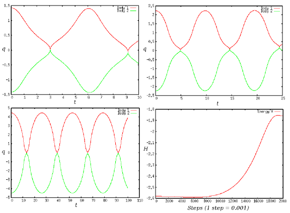
Figure 5: Some numerical integrations of the regularized system with almost symmetric initial conditions: $(Q_{1}=1,Q_{2}=0.01,P_{1}=0,P_{2}=0)$ (up-left), $(Q_{1}=5,Q_{2}=0.01,P_{1}=0,P_{2}=0)$ (up-right) and $(Q_{1}=20,Q_{2}=0,P_{1}=0,P_{2}=0)$ (down-left). The value of the mass is $m=10^{-5}$. For mid-term computations, the error in total energy grows quadratically suspected by the quadratic rescaling function and the non-separability of the regularized system (down-right).

Awknowledgments

We would like to thank the referees for their careful review, the valuable comments and the references [21, 22, 23] about algorithmic regularization. The first author is greatful to Profr. Laskar and the IMCCE for the facilities to perform the numerical computations.

References

References

• [1] R. Abraham and J. Marsden, Foundations of Mechanics, 2nd Ed., Add.-Wesl. Pub., New York, 1987.
• [2] R. Abraham, J. Marsden and T.Ratiu, Manifolds, Tensor Analysis and Applications, 2nd Edition, Appl. Math. Sci., 75, Springer-Verlag, 2003.
• [3] T. Bartsch, The Kustaanheimo-Stiefel transformation in geometric algebra, arXiv:physics/0301017v1, 10Jan2003.
• [4] T. Bountis and K.E. Papadakis, The stability of vertical motion in the $N$-body circular Sitnikov problem, Celestial Mechanics and Dynamical Astronomy 104, (2009), 205-225.
• [5] A. Celletti, Singularities, Collisions and Regularization Theory, Lectures Notes in Physics 590, Benest and C. Froeschlé (eds), Singularities in Gravitational Systems, Springer, 2002, pp. 1-24.
• [6] C. Conley and R. Easton, Isolated invariant sets and isolating blocks, Trans. Amer. Math. Soc., June, 1971.
• [7] R. Easton, Regularization of Vector Fields by Surgery, Journal of Differential Equations 10, 1971, pp 91-99.
• [8] M. Gastineau and J. Laskar, 2010. TRIP 1.1a10, TRIP Reference manual. IMCCE, Paris Observatory. http://www.imcce.fr/trip/.
• [9] Y. Hagihara, Celestial Mechanics, Japan Society for the Promotion of Science, Tokyo, Vol IV, Part 1, 1975.
• [10] H. Jiménez-Pérez, L. Franco, Symplectic Regularization On $T^{*}\mathbb{R}^{3}$, in preparation.
• [11] H. Jiménez-Pérez, E. Lacomba, On the periodic orbits of the double Sitnikov problem, C. R. Acad. Sci. Paris, Ser. I, 347, (2009), 333-336.
• [12] H. Jiménez-Pérez, El problema de Sitnikov con 4 cuerpos, Doctoral Dissertation, UAM-Iztapalapa, México City (2010).
• [13] H. Jiménez-Pérez and E. Lacomba, Energy Levels of Periodic Solutions of the Circular 2+2 Sitnikov problem, Qual. Theory Dyn. Syst. 8, No 1, (2009), 1-23.
• [14] H. Jiménez-Pérez, Complex Regularization of the Circular $N$+1 Body Problem in the Plane, preprint.
• [15] P. Kustaanheimo, E. Stiefel, Perturbation theory of Kepler motion based on spinor regularization J. Reine Angew. Math 218, (1965), 204-219.
• [16] J. Laskar, P. Robutel High order symplectic integrators for perturbed Hamiltonian systems, Celestial Mechanics and Dynamical Astronomy, 80, (2001), 39-62.
• [17] T. Levi-Civita, Sur la résolution qualitative du probléme restreinte de trois corps, Acta Mathematica 80, (1906), 305-327.
• [18] M. Lindow, Eine Transformation für das Problem der n+1 Körper, Astronomische Nachrichten Nr. 5241, Band 219, Münster, 1923, 141-154.
• [19] C. Marchal, Regularization of the Singularities of the $N$-Body Problem, NATO Advanced Study Institute Series, Math. and Phys. Sci. 82, (1981), 201-236.
• [20] M. Marchesin, The Mass Dependence of the Period of the Periodic Solutions of the Sitnikov Problem, Discrete and Continuous Dynamical Systems Series S Vol. 1, No 4 (2008), 597-609.
• [21] S. Mikkola, K. Tanikawa, Algorithmic regularization of the few-body problem, Mon. Not. R. Astron. Soc. 310, (1999), 745-749.
• [22] S. Mikkola, K. Tanikawa, Explicit Symplectic Algorithms For Time‐Transformed Hamiltonians, Celestial Mechanics and Dynamical Astronomy 74, (1999), 287-295.
• [23] M. Preto, S. Tremaine, A Class of Symplectic Integrators with Adaptive Time Step for Separable Hamiltonian Systems The Astronomical Journal, Vol 118, No. 5, (1999), 2532-2541.
• [24] C.L. Siegel, J.K. Moser Lectures on Celestial Mechanics Springer-Verlag, (1971).
• [25] L. Stiefel and G. Scheifele Linear and Regular Celes. Mechs., Springer-Verlag, (1971).
• [26] V. Szebehely, Theory of Orbits, Academic Press, New York, (1967).
• [27] M. D. Vivarelli, The K-S transformation in Hypercomplex form, Celestial Mechanics 29, (1983), 45-50.
• [28] O. Volk, Concerning the derivation of the KS-transformation, Celestial Mechanics 8, (1973), 297-305.
• [29] J. Vrbik, Perturbed Kepler problem in quaternionic form, J. Phys. A: Math. Gen. 28, (1995), 6245-6252.
• [30] J. Waldvogel, Quaternions and the perturbed Kepler problem, Celestial Mechanics and Dynamical Astronomy 95, (2006), 201-212.
• [31] J. Waldvogel, Quaternions for regularizing Celestial Mechanics: the right way, Celestial Mechanics and Dynamical Astronomy 102, (2008), 149-162.