A Novel Approach for Compression of Images Captured using Bayer Color Filter Arrays

Abstract

We propose a new approach for image compression in digital cameras, where the goal is to achieve better quality at a given rate by using the characteristics of a Bayer color filter array. Most digital cameras produce color images by using a single CCD plate, so that each pixel in an image has only one color component and therefore an interpolation method is needed to produce a full color image. After the image processing stage, in order to reduce the memory requirements of the camera, a lossless or lossy compression stage often follows. But in this scheme, before decreasing redundancy through compression, redundancy is increased in an interpolation stage. In order to avoid increasing the redundancy before compression, we propose algorithms for image compression in which the order of the compression and interpolation stages is reversed. We introduce image transform algorithms, since uninterpolated images cannot be directly compressed with general image coders. The simulation results show that our algorithm outperforms conventional methods with various color interpolation methods in a wide range of compression ratios. Our proposed algorithm provides not only better quality but also lower encoding complexity because the amount of luminance data used is only half of that in conventional methods.

I Introduction

Digital cameras use image-processing tools, e.g., interpolation techniques, such as those used in analog camcorders, in order to achieve good quality images. One big difference between digital cameras and analog camcorders is that digital cameras store digital data in flash memories. Thanks to storing digital data, functionalities such as image editing and enhancement can be added. But the price of flash memories is still very high, so that low image bit-rates are required in order to enable storage of large number of images at a reasonable cost. To achieve this, most digital cameras use lossy compression schemes like JPEG [1] to store the images.

In this paper, we focus on the color interpolation process that is used in many cameras, and specifically on how this interpolation should be taken into consideration when designing image compression for digital cameras. In order to produce full color images, most digital cameras place color filters on monochrome sensors. While some high-end digital cameras use three CCD plates to get full color images, where each plate takes one color component, most digital cameras use a single CCD plate, with several different color filters, and produce full color images by using an interpolation technique. Although there are several different color filter arrays (CFA) [2] [3], in this paper, we focus on the Bayer CFA which is most widely used in digital cameras. The Bayer CFA, as shown in Fig. 1, uses 2 by 2 repeating patterns (RP) in which there are two green pixels, one red and one blue. There is only one color component in each pixel, so the other two color components for a given pixel have to be interpolated using neighboring pixel information. For example, in a bilinear interpolation method, the red (blue) color component on a green pixel in Fig. 1 is produced by the average value of two adjacent red (blue) pixels. Although there are several possible interpolation algorithms [4] [5] [6] [7] [8] [9], it is clear that from an information theoretic viewpoint they all result in an increase of redundancy.

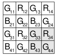
Figure 1: Bayer color filter array. Each letter indicates the position of a different color filter. R, G and B are for Red, Green and Blue, respectively. The gray block indicates 2 by 2 repeating pattern.

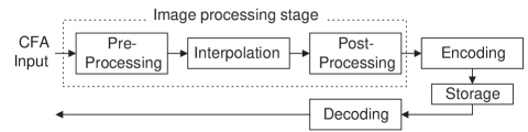
(a)

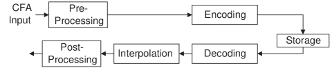
(b)

Figure 2: Block diagrams of (a) the conventional method and (b) the proposed method. In (a) an image processing stage is followed by a compression stage. In (b) interpolation and post-processing in an image processing stage are done after compression and decompression.

In a conventional method, as shown in Fig. 2 (a), after finishing the image processing stage, a lossless or lossy image compression algorithm is used before storing the image. Although in theory one could achieve the same compression with or without the interpolation, to do so would require exploiting the specific characteristics of the interpolation technique within the compression algorithm, which is clearly not easy to achieve if we wish to use a standard compliant compression method without modification. For this reason, in this paper we propose image transform algorithms to encode the image before interpolation, so that interpolation is performed only after decoding. We call this approach Interpolation after Decoding (IAD), see Fig. 2 (b). There are some other functions, such as white balancing and color correction, that are performed in the image processing stage. These are shown as pre- and post-processings in the figure. In our proposed approach less data needs to be encoded, since only one color is available at each pixel position before interpolation. The main challenge is then how to organize the available data for encoding in order to best exploit the spatial redundancy for compression.

Methods to use increase image quality using the redundancy of interpolation in post- and pre-processing stages and using encoder characteristics during interpolation have been studied. In [10], under the assumption of a fixed interpolation algorithm, the quantization noise is reduced by using an iterative method that incorporates information about the interpolation algorithm. By contrast our approach assumes only a specific CFA and can operate with any interpolation technique. The main difference is that our algorithms compress non-interpolated images without introducing the redundancy of interpolation, whereas the algorithm in [10] improves image quality by exploiting the redundancy of interpolation.

In [11], under a given compression method, minimizing error between a decoded full color source and a decoded image after interpolation is studied, but the complexity required is too high to use in digital cameras. In [12], as a modified approach of our previous work in [13], CFA data compression with different format conversion is proposed but the method is limited to work with bilinear interpolation. Since in our algorithm, interpolation is not involved in encoding and decoding processes, the algorithm itself is independent from interpolation methods. Also, interpolation is done on the decoded pixels and so any interpolation method which is not sensitive to the coding error can be applied.

As an image coder, JPEG is widely used in digital cameras because it is relatively simple and provides good performance, especially when the compression ratio is low. JPEG is a block discrete cosine transform (DCT) based coder and the blocking artifacts can become severe as the compression ratio becomes higher. Discrete wavelet transform (DWT) based coders such as EZW [14], SPIHT [15] and EBCOT [16] (adopted in JPEG2000 [17]) are also used as image coders. A DWT based coder does not produce blocking artifacts and it provides good performance at high compression ratios. In this paper, we use JPEG and SPIHT as representative of the DCT and DWT based approaches, respectively. Our proposed algorithms are tested under both of these coding techniques. Although we focus on standard compression methods, interpolation aware compression methods can provide better performance especially when the interpolation method used is sensitive to the coding error of standard compression methods.

In this paper, extending our previous work in [13], we propose several different algorithms to transform the non-interpolated images before compression. We provide performance results of the proposed algorithms with different coders (JPEG and SPIHT) and interpolation methods (bilinear and adaptive interpolation). Also, using a simple example based on one-dimensional data, we propose an analysis to provide some intuition about why our approach outperforms conventional compression-after-interpolation (CAI) methods. In our problem an original full color image is not available, since cameras are assumed to capture images with single color pixels. Thus, for the purpose of comparison we use as a reference a full color image obtained by interpolating the original (uncompressed) captured image. Therefore our problem will be to find coding schemes that are optimized in terms of minimizing the error with respect to that original interpolated image. The experimental results show that the proposed algorithms outperform the conventional method in the full range of compression ratios for JPEG coding with bilinear interpolation and up to 20 : 1 or 40 : 1 compression ratio for SPIHT coding depending on the interpolation methods used. Thus, in both cases, our proposed techniques are superior in the range of compression ratios that are used in practical digital cameras (i.e., those corresponding to high quality images).

This paper is organized as follows: in Section II, the theoretical rate distortion performance of the CAI and IAD approaches is analyzed by using a 1-D sequence and DPCM encoding. Proposed image transform algorithms are addressed in Section III. Experimental results are provided as demonstration of the validity of our algorithm in Sections IV and V. Finally, the conclusion of this work is in Section VI.

II Performance comparison using one dimensional sources

The main difference between the CAI and IAD methods is the order of compression and interpolation. In this section we propose an analysis to provide some intuition about why an IAD method can theoretically outperform a CAI method by considering differential pulse code modulation (DPCM) compression of a one dimensional first order autoregressive (AR) process. DPCM exploits the correlation between two adjacent pixels to reduce the residual energy coded, whereas transform coding used in standard image coding exploits spacial correlation to pack a large fraction of its total energy in relatively few transform coefficients. Therefore DPCM compression has similar coding process (including decorrelation, quantization and entropy coding) to standard image coding, although the performance of decorrelation in DPCM is weaker than that in transform coding.

First, we compare the R-D performance of DPCM and DPCM after interpolation (DPCMI). Then, we show that the IAD method outperforms the CAI method under the following assumptions: (i) DPCM coding is used, (ii) the interpolated sequence is divided into two sub-sequences during coding and (iii) the distortion is measured after interpolation.

Although open loop DPCM is not generally used due to the error propagation in the decoded sequence, its analysis is easier, given that the difference sequence has an explicit theoretical R-D curve when the source is a Gaussian AR process.

(a)	(b)

Figure 3: Gray and white boxes indicate original and interpolated samples, respectively. In (a), $\{Z_{n}\}$ is a differential sequence of the original sequence taken from sensors and in (b), $\{T_{n}\}$ and $\{S_{n}\}$ indicate a differential sequence of the interpolated sequence.

Therefore we consider open loop DPCM of one dimensional first order zero mean Gaussian AR processes. Let

$$X_{n}{}={}\rho X_{n-1}{}+{}W_{n},~{}n=1,2,\cdots,$$ (1)

denote the process, where $\{W_{n}\}$ is a zero-mean sequence of independent and identically distributed random variables and $W_{n}\sim N(0,\sigma_{W}^{2})$, and $\rho$ is the correlation coefficient ($0\leq\rho<1$). Then from the probability distribution of $W_{n}$, the probability distribution of $X_{n}$ is $N(0,\sigma_{W}^{2}/(1-\rho^{2}))$. We assume that the initial state $X_{0}$ is given and we are interested in the source outputs for $~{}n\geq 1$.

We define the differential sequence of $\{X_{n}\}$ as $\{Z_{n}\}$

$$Z_{n}\triangleq X_{n}-X_{n-1}\\ {}={}(\rho-1)X_{n-1}{}+{}W_{n}~{}.$$ (2)

Since $X_{n-1}$ and $W_{n}$ are independent, $Z_{n}$ also has Gaussian distribution ($Z_{n}\sim N(0,~{}2\sigma_{W}^{2}/(1+\rho))$).

The rate distortion (R-D) function for a Gaussian source with mean square error (MSE) distortion can be written in closed form [18] and therefore the R-D function of ${Z_{n}}$ is

$$R_{1}(D)=\frac{1}{2}\log_{2}(\frac{2\sigma_{W}^{2}}{(1+\rho)D}),~{}~{}~{}~{}\text{for }0\leq D<\frac{2\sigma_{W}^{2}}{1+\rho}~{},$$ (3)

where $D$ denotes average distortion of the data coded. The distortion of interpolated pixels is addressed in the last part of this section.

Next, we double the number of samples by using a linear interpolation method and define this new sequence $Y_{n}$ as :

$$\begin{cases}Y_{2n}\triangleq X_{n},\\ Y_{2n+1}\triangleq(X_{n}+X_{n+1})/2.\end{cases}$$ (4)

From this sequence, as shown in Fig. 3 (b), two differential sequences $\{T_{n}\}$ and $\{S_{n}\}$ can be defined as

$$\begin{cases}T_{n}\triangleq Y_{2n-1}-Y_{2n-2}\\ S_{n}\triangleq Y_{2n}-Y_{2n-1}.\end{cases}$$ (5)

Note that because of the chosen interpolation mechanism, $T_{n}$ is identical to $S_{n}$ (i.e., $T_{n}=S_{n}=(X_{n}-X_{n-1})/2$) and the probability distribution of $T_{n}$ (or $S_{n}$) is $N(0,\sigma_{W}^{2}/2(1+\rho))$. Since both $\{T_{n}\}$ and $\{S_{n}\}$ are Gaussian sources, their R-D functions are :

$$R_{T}(D)=R_{S}(D)=\frac{1}{2}\log_{2}(\frac{\sigma_{W}^{2}}{2(1+\rho)D}),~{}\text{for }0\leq D<\frac{\sigma_{W}^{2}}{2(1+\rho)}~{}.$$ (6)

In this example, since $S_{n}$ and $T_{n}$ are same, there is no need to encode $S_{n}$ if $T_{n}$ is available. However, in our original problem, the difference of neighboring pixels of interpolated images is not same since more than two pixels are involved in 2-D interpolation. Also, a standard compliant compression algorithm cannot employ additional information related to interpolation. Therefore, although $S_{i}$ and $T_{j}$ can be spatially correlated, we assume that $S_{i}$ and $T_{j}$ will be encoded independently for all $i$ and $j$. Then the rate distortion function of DPCM for $Y_{n}$, i.e., the R-D function for the DPCMI approach, will be :

$$R_{2}(D)=R_{T}(D)+R_{S}(D)=\log_{2}(\frac{\sigma_{W}^{2}}{2(1+\rho)D}),~{}\text{for }0\leq D<\frac{\sigma_{W}^{2}}{2(1+\rho)}~{}.$$ (7)

Figure 4: The upper (lower) graph is for $\rho=0.9$ ($\rho=0.1$). Solid lines indicate the R-D curve of the differential sequence ($\{Z_{n}\}$) and dotted lines indicate the R-D curve of the differential sequences after interpolation ($\{S_{n}\}$ and $\{T_{n}\}$).

The main difference between above two methods (DPCM and DPCMI) is the number of samples to be coded and the variance of the respective sequences. The number of samples encoded by DPCM is half the number encoded by DPCMI, while DPCM encodes a sequence with 4 times larger variance than that encoded by DPCMI. There is a clear trade-off between the two methods since reducing the number of samples will tend to reduce the rate, while increasing variance will tend to increase the rate per sample. Fig. 4 compares the performance of the two methods with different AR coefficients. In the figure, the performance of DPCM is better than that of DPCMI at higher rates but is worse at lower rates. This shows that at high rates having to encode fewer samples (DPCM) is better, even though the variance of those samples is higher. The trade-off is reversed at low bit rates. Intuitively, DPCM starts to have an error at lower bit-rate than DPCMI due to the smaller number of samples, but its error is increased faster than that of DPCMI due to the larger variance. Therefore at higher rate, the performance of DPCM is better and it can be worse at lower rate.

Instead of theoretical R-D curves, we now consider operational R-D curves of general DPCM coders that use a uniform quantizer and an entropy coder. We assume that a given quantizer has $N$ quantization bins. In the DPCM system, let each bin size be $\Delta$ (except top and bottom bins assuming that the range of source is infinite), let the average MSE be $d$ and, after entropy coding, let the average rate be r. Then, in the DPCMI system, each bin size can be $\Delta/2$ and the average MSE is $d/4$ for $T_{n}$ since the maximum sample value of $T_{n}$ is half the maximum value for $Z_{n}$. This is because $T_{n}=(X_{n}-X_{n-1})/2=Z_{n}/2$. However the number of samples in a given bin is exactly same as that in a corresponding bin of $Z_{n}$, so the rate is still $r$ after applying the same entropy coder. Therefore, if the R-D curve of DPCM passes a point $(r,d)$ then that of DPCMI passes a point $(2r,d/4)$ (note that $T_{n}$ and $S_{n}$ each have rate $r$ in the DPCMI system). This relation is formulated as

$$G(d)=\frac{1}{2}H(\frac{d}{4}),$$ (8)

where $G$ and $H$ are the R-D functions of DPCM and DPCMI, respectively. This also indicates that in general there will be a trade-off point between the CAI and IAD approaches.

In (3), the R-D function is determined by ${Z_{n}}$ (i.e., the coefficients in a DPCM domain corresponding to a non-interpolated sequence) and this is not equivalent to the R-D function of the IAD method (in which the R-D function is determined by the interpolated sequence after decompression). In order to evaluate the performance of the IAD method, we first need to know the R-D performance of the source sequence. The R-D performance of the difference sequences (generated by open loop DPCM system) may not be same that of source sequences since the decoder only has a quantized version of previous sample values. But, in the orthogonal (or approximately orthogonal) transform coding case, which is more relevant for image coding (i.e., DCT or DWT), the distortion in the transform domain is the same as or close to that in a pixel domain depending on the transform . Therefore the approximation used in open loop DPCM is not required and so the analysis approximately holds. The following shows that in the IAD method, the average MSE can be decreased after interpolation. Let us assume that the average MSE of the reconstructed sequence ($\{\hat{X}_{n}\}$) before interpolation is $d$ then the sample interpolated between $\hat{X}_{n}$ and $\hat{X}_{n+1}$ is $(\hat{X}_{n}+\hat{X}_{n+1})/2$, and its average MSE satisfies

$$E(\frac{\hat{X}_{n}+\hat{X}_{n+1}}{2}-\frac{X_{n}+X_{n+1}}{2})^{2} {}={}E(\frac{(\hat{X}_{n}-X_{n})^{2}+(\hat{X}_{n+1}-X_{n+1})^{2}}{4})$$ (9)

$$~{}~{}~{}~{}{+}E(\frac{(\hat{X}_{n}-X_{n})\cdot(\hat{X}_{n+1}-X_{n+1})}{2})$$

$${}\leq{}\frac{E(\hat{X}_{n}-X_{n})^{2}+E(\hat{X}_{n+1}-X_{n+1})^{2}}{2}$$

$${}={}d~{}\text{.}$$

In (9), inequality comes from

$$E((\hat{X}_{n}-X_{n})\cdot(\hat{X}_{n+1}-X_{n+1})){}\leq{}\frac{E(\hat{X}_{n}-X_{n})^{2}+E(\hat{X}_{n+1}-X_{n+1})^{2}}{2}~{}\text{.}$$ (10)

Equality holds only when $E((\hat{X}_{n}-X_{n})-(\hat{X}_{n+1}-X_{n+1}))^{2}=0$ (i.e., if the error of two reconstructed pixels is same then the error of the interpolated pixel is same as the reconstructed pixel). If the error of $\hat{X}_{n}$ (i.e., $\hat{X}_{n}-X_{n}$) and $\hat{X}_{n+1}$ is uncorrelated and has zero mean then the average MSE of the interpolated pixel is $d/2$. Therefore average distortion can be decreased after interpolation. This means interpolated pixels are not necessarily considered during performance analysis (since their distortion is always smaller than or equal to that of pixels coded), and so the analysis based on $R_{1}(D)$ and $R_{2}(D)$ is still valid for the interpolated sequence. Also, under the assumption that the R-D functions of DPCM and pixel domains are similar, the IAD method provides better performance in a larger range of different compression ratios.

In a 2-D case, ${X_{n}}$ and ${Y_{n}}$ can be considered as non-interpolated and interpolated images, respectively. Since transforms, rather than DPCM, are typically used for images, we can consider ${Z_{n}}$ and ${T_{n}}$ (and ${S_{n}}$) to represent the coefficients in the transform domain of the non-interpolated and interpolated images, respectively. Although the order of the process is same between 1-D and 2-D cases, our analysis of the 1-D sequence may not be directly applied to a 2-D case since each function in the process is not same. But, we can expect that the IAD method outperforms at very high rates (at least, until the rates are higher than the rates required for the IAD method without compression) since the IAD method uses around half the amount of data. Also, in the IAD method, images may have larger variance, since it has weaker spatial correlation due to larger distance between adjacent pixels. So, similar to the result in the 1-D case (shown in Fig. 4), the R-D curve of the IAD method drops more sharply than that of the CAI method. Therefore, the R-D curves of IAD and CAI methods may be crossed as bit-rate is decreased, and depending on the location of the cross point, the IAD method can provide better performance in practical applications such as digital cameras.

III IMAGE TRANSFORM TO REDUCE REDUNDANCY

In order to demonstrate a practical IAD scheme our first goal is to transform the non-interpolated input data into a format suitable for general image coders. The input data of the IAD method consists of only one color value for each pixel, while in the CAI method there are three color values for each pixel, obtained by interpolation. In general image coders, it is assumed that incoming data is uniform (i.e., all pixels have the same color components) and that the image has rectangular shape. Our goal is then to design a reversible image transform that can produce image data suitable for coding (without increasing the amount of data to be coded). A detailed diagram of the encoding and decoding blocks of the IAD method is shown in Fig. 5.

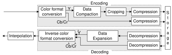
Figure 5: Detailed diagram of the encoding and decoding parts of the proposed IAD method. Luminance (Y) data needs several transforms due to data location after format conversion, whereas chrominance (Cb/Cr) data can be coded directly.

First, we propose a color format conversion algorithm, since image coders normally use YCbCr format. After format conversion, luminance (Y) data is not available at every pixel position. In order to make the Y data compact, we propose a transform that relocates pixels and removes pixels for which no Y data is available. Then we show how to encode the resulting data which no longer has rectangular shape.

III-A Color format conversion

In the CAI method, the data to be compressed is in RGB format (obtained by interpolating the CFA data). This data is converted to YCbCr format before compression. In JPEG, normally 4:2:2 or 4:2:0 sampling is used. In JPEG2000, chrominance coefficients in high frequency bands after wavelet transform are not coded since the human visual system is less sensitive to the chrominance data. In the IAD method, to avoid increasing the redundancy, the number of pixels should not be increased after color format conversion. While there are several different methods to achieve this, we choose a method such that 2 green, 1 red and 1 blue pixels are converted to 2 Y, 1 Cb and 1 Cr pixel values. This is reasonable since luminance data is more important than chrominance data and the format conversion can be reversible. We first propose a simple and fast method based on 2 by 2 blocks and then propose more complex methods that provide better performance.

III-A1 Format conversion based on 2 by 2 blocks

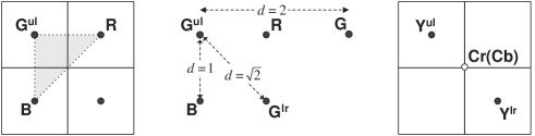
(a)                        (b)                       (c)

Figure 6: The gray region in (a) indicates the possible location of Y data after the format conversion. (b) shows the distance between two green (or luminance) pixels. (c) shows the location of Y and Cr (Cb) data in a 2 by 2 block.

In this format conversion, each 4 pixel block contains 2 green, 1 red and 1 blue pixels. Then two luminance and two chrominance values (i.e., Cb and Cr) are obtained by using one green pixel for each of the two luminances, and using the average of the two green pixels for the chrominance calculation. This operation can be represented as follows :

$$\left[\begin{array}[]{c}Y^{ul}\\ Y^{lr}\\ Cb\\ Cr\end{array}\right]=\left[\begin{array}[]{clcr}a_{11}&a_{12}&0&a_{13}\\ a_{11}&0&a_{12}&a_{13}\\ a_{21}&\frac{a_{22}}{2}&\frac{a_{22}}{2}&a_{23}\\ a_{31}&\frac{a_{32}}{2}&\frac{a_{32}}{2}&a_{33}\end{array}\right]\left[\begin{array}[]{c}R\\ G^{ul}\\ G^{lr}\\ B\end{array}\right]+\left[\begin{array}[]{c}0\\ 0\\ 128\\ 128\end{array}\right],$$ (11)

where, as shown in Fig. 6 (b) and (c), the superscripts $ul$ and $lr$ indicate the upper left and lower right positions in a 2 by 2 CFA block, respectively. The coefficients $a_{ij}$ are the (i,j) coefficients of the standard RGB to YCbCr conversion matrix [19] defined as follows:

$$\left[\begin{array}[]{c}Y\\ Cb\\ Cr\end{array}\right]=\left[\begin{array}[]{clcr}0.297&0.587&0.114\\ -0.169&-0.331&0.500\\ 0.500&-0.419&-0.081\end{array}\right]\left[\begin{array}[]{c}R\\ G\\ B\end{array}\right]+\left[\begin{array}[]{c}0\\ 128\\ 128\end{array}\right]$$ (12)

We now need to decide what the location of these $Y^{ul}Y^{lr}CbCr$ pixels should be. For the $Cb$ and $Cr$ data, each component could be located in any fixed position in the 2 by 2 block, since only one value of each chrominance is generated for the block. In the Y data case, however, one ($Y^{ul}$) should be located in the upper left region since $Y^{ul}$ is the weighted average of $G^{ul}$, $R$ and $B$ (as shown in Fig. 6 (a)) and the other ($Y^{lr}$) should be located in the lower right region of the block.

In our algorithm, we put the Y data at each green pixel position because green is roughly 60% of the Y data (the shape of the Y image is shown in Fig. 7 (a)). The location of the Y data is important, since improperly located Y data induces artificial high frequency components which can degrade the coding performance.

This method is simple and fast but YCbCr data of each 2 by 2 block depends only on the RGB data in that 2 by 2 block. Therefore, the YCbCr data potentially has more high frequency components than that generated by using bilinear interpolation (because each block is treated independently, while in the bilinear interpolation case each Y term is obtained from a larger set of pixels).

III-A2 Format conversion based on larger blocks

In order to generate smoother YCbCr data, we can consider a whole image as a block. After generating the RGB data for each pixel by using bilinear interpolation, Y, Cb and Cr can be calculated from the RGB data on green, blue and red pixels respectively. These positions are chosen according to the degree of influence of each color (i.e., the dominant color components of Cb and Cr are blue and red, respectively). Although each pixel has RGB data after interpolation, the amount of YCbCr data is not increased, since each pixel position has only one component, either Y, Cb or Cr. This format conversion is also simple but the reverse format conversion is more complex due to bilinear interpolation. For example, as in Fig. 1, we consider that the image size is 4 by 4. Then $Y_{22}$ (the luminance value of the $G_{22}$ position) is calculated as

$$\begin{split}Y_{22}&=\left[0~{}~{}\frac{a_{11}}{2}~{}~{}0~{}~{}0~{}~{}\frac{a_{13}}{2}~{}~{}a_{12}~{}~{}\frac{a_{13}}{2}~{}~{}0~{}~{}0~{}\frac{a_{11}}{2}~{}~{}0~{}~{}0~{}~{}0~{}~{}0~{}~{}0~{}~{}0\right]\\ &\quad\cdot\left[G_{11}~{}R_{12}~{}G_{13}~{}R_{14}~{}B_{21}~{}G_{22}~{}B_{23}~{}G_{24}~{}G_{31}~{}R_{32}~{}G_{33}~{}R_{34}~{}B_{41}~{}G_{42}~{}B_{43}~{}G_{44}\right]^{T}~{}\text{.}\end{split}$$ (13)

But, in the reverse format conversion, $G_{22}$ is calculated as

$$\begin{split}G_{22}&=\left[\text{\small{-1243 ~{}-3832~{}-1079~{}217~{}-1763~{}14895~{}-1736~{} -135~{}-974~{}-3658~{}-868~{}136~{}35~{}-638~{}26~{}37}}\right]\cdot 10^{-4}\\ &\quad\cdot\left[Y_{11}~{}Cr_{12}~{}Y_{13}~{}Cr_{14}~{}Cb_{21}~{}Y_{22}~{}Cb_{23}~{}Y_{24}~{}Y_{31}~{}Cr_{32}~{}Y_{33}~{}Cr_{34}~{}Cb_{41}~{}Y_{42}~{}Cb_{43}~{}Y_{44}\right]^{T}~{}\text{.}\end{split}$$ (14)

From the example of (13) and (14), we can see that in general the forward format conversion may be based on a few neighboring pixels but reverse conversion could require all pixels in the same block. Therefore, in order to generate the original RGB data from the YCbCr data, a $w\cdot h$ by $w\cdot h$ reverse format conversion matrix is needed, where $w$ and $h$ are the width and height of an image respectively.

Although the decoding process (including reverse format conversion) can be done in a system with high computing power (e.g., personal computers), the matrix is too large and the reverse conversion may still be too time consuming. In order to reduce the computational complexity, the above format conversion method can be applied to blocks generated by dividing the source image. Since interpolation is done by using the pixels in the block, the column (or row) of the reverse format conversion matrix is reduced to $W\cdot H$, where $W$ and $H$ are the width and height of a block respectively. In this block based format conversion, the bilinear interpolation needs to be modified since only the information of pixels in the same block can be used for interpolation. For example, the green value on $(i,j)$ position (which corresponds to a red or blue pixel position) can be calculated as

$$G_{ij}=~{}\frac{G^{\prime}_{(i-1)j}+G^{\prime}_{(i+1)j}+G^{\prime}_{i(j-1)}+G^{\prime}_{i(j+1)}}{I_{(i-1)j}+I_{(i+1)j}+I_{i(j-1)}+I_{i(j+1)}},$$ (15)

where $G^{\prime}_{kl}=I_{kl}\cdot G_{kl}$, and $I_{kl}$ is an indicater function defined as follows.

$$I_{kl}=\begin{cases}1,&~{}\text{if $kl$ and $ij$ are in the same block}\\ 0,&~{}\text{otherwise.}\\ \end{cases}$$ (16)

Then $G_{ij}$ is used to calculate $Cb_{ij}$ (or $Cr_{ij})$ at the blue (or red) position.

Note that, in the decoding process, an approximation method which uses only neighboring pixels can be used since more distant pixels do not have a big influence (see the coefficients in (14)). But in this paper, we focus on a block-based method in order to avoid the effect of error in format conversion.

The performance comparison among different block size format conversion is given in Section IV-A.

III-B Nonlinear transform to compact luminance data

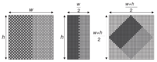
(a)                      (b)                      (c)

Figure 7: Transform of Y (luminance) image. In the figure, dark and light gray pixels indicate Y data and white pixels indicate empty position. (a) indicates quincunx located Y image after format conversion, (b) and (c) indicate Y image after transform. In (b), each odd column data is shifted to the left even column and in (c), each pixel is rotated 45 degree clockwise.

After the color format conversion, the Y values are not available at all the original pixel positions (since the Y data is located only in the position of the green pixels), so general image compression methods cannot be directly applied to compress the Y image. Therefore another reversible transform is needed to change the Y pixels located on a quincunx lattice (see Fig. 7 (a)) to normally located Y pixels (i.e., so that we obtain a Y image with no blank pixels). As in Fig. 7 (b), one possible simple transform is a horizontal pixel shift where pixels in odd columns are shifted to the left even column and all odd columns are removed. This transform can be formulated as

$$if~{}x+y=odd,~{}\left[\begin{array}[]{c}X\\ Y\end{array}\right]=\begin{cases}~{}\left[~{}~{}\begin{array}[]{c}{\frac{x}{2}}\\ y\end{array}~{}~{}\right],~{}if~{}x=even,\\ ~{}\left[\begin{array}[]{c}{\frac{x-1}{2}}\\ y\end{array}\right],~{}if~{}x=odd,\end{cases}$$ (17)

where $(x,y)$ and $(X,Y)$ are the pixel positions in the images before and after transform, respectively. Here we assume that the origin is the lower left corner of an image. A vertical shift transform can be similarly defined, but we focus here on the horizontal shift transform.

After the transform is performed, a vertical edge (e.g., Fig. 7 (b)) leads to artificial high frequency components in the vertical direction, which leads to coding performance degradation. This also happens when the edge is vertically biased (i.e., steeper than a 45 degree line). Note that if a vertical shift had been chosen the same problem would arise with respect to horizontal (and horizontally biased) edges. Thus, under JPEG coding with a high compression ratio, most of this artificial high frequency information may be lost. Spatially weak correlation is another reason that contributes to making the results worse. If the distance between adjacent pixels in a row (or a column) in a CFA is assumed to be 1 then, after horizontal shifting, the vertical and horizontal distances of adjacent pixels in the Y data are $\sqrt{2}$ and $2$ respectively (see Fig. 6 (b)).

An alternative simple transform to remove blank pixels among Y data, which does not pose these problems, is a 45 degree rotation formulated as

$$\begin{split}\left[\begin{array}[]{c}X\\ Y\end{array}\right]=\frac{1}{2}\left(\left[\begin{array}[]{clcr}1&1\\ -1&1\end{array}\right]\left[\begin{array}[]{c}x\\ y\end{array}\right]+\left[\begin{array}[]{c}-1\\ w-1\end{array}\right]\right),\\ ~{}~{}\text{for }x+y=odd,\end{split}$$ (18)

where $w$ indicates the image width. As shown in Fig. 7 (c), after rotation, Y data is concentrated on the center of an image with an oblique rectangular shape. This transform does not induce artificial high frequencies and the distances between adjacent pixels in a row or column are now $\sqrt{2}$. But since the data no longer has a standard rectangular shape area, some redundancy is added when the boundary pixels are coded. This is addressed in the next section and the performance comparison between shift and rotation transform is presented in Section IV-B.

As shown in (17) and (18), the complexity of both methods is low. The rotation method needs 1 comparison, 2.5 addition and 1 shift operation per pixel whereas the shift method needs 1.5 comparison, 1.25 addition and 0.5 shift operation.

III-C Data cropping for images obtained by the rotation transform

After the horizontal shift transform (see Fig. 7 (b)) Y data can be directly encoded. But the shape of Y data after the rotation transform is not rectangular (see Fig. 7 (c)) and thus coding the shape bounding box (i.e., the whole rectangular region that includes the oblique rectangular shape of Y data) would result in some inefficiency in the coding. Therefore a proper cropping method is needed to remove the data outside of the oblique rectangular area containing Y data.

III-C1 Data cropping for JPEG (DCT based coders)

In JPEG, the size of a DCT block is 8 by 8 and blocks that consist of blank pixels only (blank blocks) do not need to be coded. In addition, we do not need to send any side information about the location of Y data since it can be calculated at the decoder given the size of the original image. As shown in Fig. 7 (c), the number of blank blocks depends on the width and height of the image and 6 bits (2 bits for a zero DC value and 4 bits for EOB (end-of-block)) are needed to code a blank block when standard Huffman tables of JPEG are employed. In case of 512 by 512 images, out of 4096 blocks, the number of blank blocks is 1984 and without coding blank blocks, we can save 1488 bytes. The blocks containing boundary pixels of Y data (boundary blocks) also contain blank pixels since Y data are in an oblique rectangular shape. As a result, compared to the shift method, the number of blocks to be coded is increased by $(w+h)/16$ in case that the width and height are multiples of 16.

Proper padding methods are needed for boundary blocks since the discontinuity between blank and data pixels in the block creates artificial edges that require a significant coding rate. Because boundary blocks have Y data only in the position of an upper or lower triangular region, padding can be simply done by diagonal mirroring using a data copy where the source data position is determined by table look-up. Four different look-up tables are needed since each boundary needs a different pattern of a data copy. Better performance can be achieved by using low-pass extrapolation (LPE) [20] or shape adaptive DCT (SA-DCT) [21][20][22]. LPE is relatively simple and provides good R-D performance whereas SA-DCT provides better performance but is more complex.

III-C2 Data cropping for SPIHT (DWT based coders)

Contrary to JPEG, SPIHT is not a block based coder and so the method used with JPEG cannot be applied. Therefore we need to introduce a new coding method in order to code Y data in the oblique rectangular area only. In the still image coding of MPEG-4, arbitrarily shaped objects are coded by using shape adaptive DWT (SA-DWT) [23]. SA-DWT uses a length adaptive 1-D DWT after finding the first non-blank pixel in the line and the low-pass (high-pass) wavelet coefficients are placed into the corresponding location in the low-pass (high-pass) band (i.e., the shape is reserved in each band after transform). One of the good features of SA-DWT is that the number of coefficients after SA-DWT is identical to the number of data pixels. In order to code data pixels only, we employ SPIHT with SA-DWT. But without modifying entropy coding in SPIHT, some redundancy is still added since SPIHT uses a two by two block arithmetic coding algorithm.

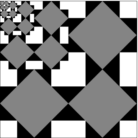
Figure 8: The coefficients map after SA-DWT (when the width and height of images are 512). Gray regions indicate meaningful coefficients and black and white regions indicate blank coefficients.

In Fig. 8, only the gray regions contain meaningful coefficients after SA-DWT. Out of 16 two by two blocks in the lowest frequency band, only 4 blocks located in each corner consist of blank coefficients. Since all descendants of these blocks (white regions in the figure) are blank coefficients, these regions are not coded. But blank coefficients in black regions in the figure are involved in coding due to the entropy coding scheme of SPIHT, and since they are not skipped some redundancy is introduced.

The complexity of the SA-DWT is no more than that of conventional DWT for the shape bounding box size image [23]. Here, the width and height of the shape bounding box are $(w+h)/2$, but the complexity is much lower since the shape is at most half the size of the shape bounding box. Also, a simpler SA-DWT method can be applied since the shape is convex. In fact, after finding the non-blank data position (which can be calculated from the width and height of the image), the complexity is about half of DWT for interpolated images. Also, in the entropy coding of SPIHT, the white region in Fig. 8 is not coded and the tree related to the black region is terminated early when all the descendent are blank coefficients.

III-D Influence of chrominance data over luminance data

In the IAD algorithms, one Cb (Cr) data is chosen out of 4 CFA pixels and the width and height of the Cb (Cr) image are $w/2$ and $h/2$, respectively. Therefore the data size is reduced to a quarter of that in the conventional technique whereas the pixel distance is doubled. But contrary to the CAI method, in which the coding results of luminance and chrominance data are fully separated, chrominance data with large distortion can add distortion to luminance data after interpolation, and vice versa.

For the case of format conversion with 2 by 2 blocks, the coding error in RGB data is calculated as follows.

$$\left[\begin{array}[]{c}e(R)\\ e(G^{ul})\\ e(G^{lr})\\ e(B)\end{array}\right]=\left[\begin{array}[]{clcr}a_{11}&a_{12}&0&a_{13}\\ a_{11}&0&a_{12}&a_{13}\\ a_{21}&\frac{a_{22}}{2}&\frac{a_{22}}{2}&a_{23}\\ a_{31}&\frac{a_{32}}{2}&\frac{a_{32}}{2}&a_{33}\end{array}\right]^{-1}\left[\begin{array}[]{c}e(Y^{ul})\\ e(Y^{lr})\\ e(Cb)\\ e(Cr)\end{array}\right],$$ (19)

where $e(\cdot)$ is the error of each component due to lossy coding. Since the final Y data (after interpolation) is calculated from the distorted RGB data, i.e., from distorted YCbCr data, the error in the final Y data depends on the quantization errors in both Y and Cb (Cr) data. For example, after applying bilinear interpolation, the error of the final Y on $G_{33}$ (in Fig. 1) is calculated as follows.

$$\begin{split}e(\tilde{Y_{33}})&=\frac{a_{11}}{2}(e(R_{32})+e(R_{34}))+a_{12}~{}e(G_{33})+\frac{a_{13}}{2}(e(B_{23})+e(B_{43}))\\ &=0.897~{}e(Y_{33})+0.075~{}(e(Y_{31})+e(Y_{42}))+0.029~{}(e(Y_{13})+e(Y_{24}))-0.103~{}e(Y_{44})\\ &~{}~{}+0.210~{}(e(Cr_{32})-e(Cr_{34}))+0.101~{}(e(Cb_{43})-e(Cb_{23})),\end{split}$$ (20)

where $\tilde{Y}$ is the final Y, and this comes from (13) and (19). In (20), the error in the final Y depends on not only the error in Y but also the error difference between two Cb (Cr) involved in the interpolation. Therefore, in order to maximize the quality of final Y and Cb (Cr) data under given bit budget, bit allocation between Y and Cb (Cr) data needs to be considered.

In SPIHT, each component is coded separately and there are no explicit mechanisms for bit allocation, whereas in JPEG bit allocation to each component cannot be explicitly controlled and is determined by the chosen quantization tables and the data characteristics. Therefore in SPIHT, it is necessary to determine the bit allocation between luminance and chrominance data based on human visual sensitivity to each component. Moreover, in the proposed methods, the bit-rate of one component affects the quality of the other components, so the overall performance changes depending on the bit allocation.

Here, we simply consider bit allocation based on the quality of luminance data since the human visual system is more sensitive to luminance data. Fig. 9 (a) shows the quality change of luminance data after interpolation depending on the overall bit-rate and the bit-rate of the luminance data. The intersection of the curves in the figure shows more bit budget for Y does not guarantee higher PSNR of Y. Also, we can find that the PSNR of Y is maximized when the bit budget of Y is roughly $80\%$ of the overall bit budget. Similarly, Fig. 9 (b) shows the quality change of chrominance data after interpolation. Although the PSNR decreases sharply, this happens in the range where the bit-rate of luminance data is lower than that of chrominance data. In general, the bit-rate of luminance data is higher than that of chrominance data and this drop does not have a significant effect. This also guarantees that we can focus on the quality of luminance data.

Since the R-D characteristics are different for each image, we fixed the bit-rate of Cb (Cr) data to be a quarter of that of Y data (i.e., $66.7\%$ of the overall budget).

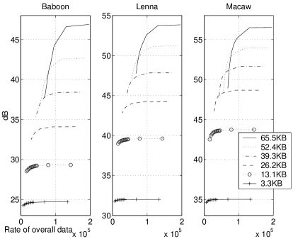
(a)

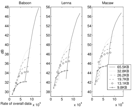
(b)

Figure 9: The curves indicate (a) luminance and (b) chrominance PSNR after interpolation depending on the overall bit-rate. SPIHT is used as a compression method and PSNR is calculated from the distortion between the interpolated image before compression and the final output image of proposed methods. The bit-rates shown in the box correspond to (a) luminance and (b) chrominance data.

IV Experimental results and discussion

In order to confirm the validity of the IAD algorithms, we implemented these algorithms (horizontal shift transform with 2 by 2 block format conversion and rotation transform with 2 by 2 and 64 by 64 block format conversion) and compared the results with those obtained with CAI (JPEG with 4:2:2 format and SPIHT) methods. Due to the lack of CFA raw data, we generate CFA raw data by using test images such as “Baboon”, “Lenna” and “Macaw” (H : 512, W : 512, 24 bit color, 786.432KB). In fact, what we obtain is not CFA raw data, since in these images all image processing functions, except interpolation, have been already done. Since our main focus has been on interpolation and compression methods, other image processing parts are not considered. Our results are the same as the results achieved when all image processing functions are done before compression and interpolation. As we mentioned in Section II, in order to compare the performance, we consider interpolated images without compression as the reference images.

The results of the proposed and conventional algorithms are compared using the PSNR of luminance (and chrominance) data and the average $\Delta{E}$ in CIELAB color space at each target bit-rate. Parts of experimental results are also shown in a webpage [24]. In the webpage, visual comparison is provided under a fixed compression ratio ($15:1$) and the difference of bit-rate under near-lossless coding is provided by using fixed PSNR (48dB). The compression ratio used in digital cameras is about $3:1$ to $20:1$ depending on vendors and user setting [25][26], and the visual difference of the results is not clearly noticeable although the IAD method provides large PSNR gain in this low compression range. But with the IAD method, same quality can be achieved with much lower bit-rate.

We first compare the performance of different color format conversion and nonlinear transform with cropping proposed in Sections III-A and III-B (III-C), respectively. After that we compare the overall performance of the IAD method to that of the CAI method.

IV-A Color format conversion

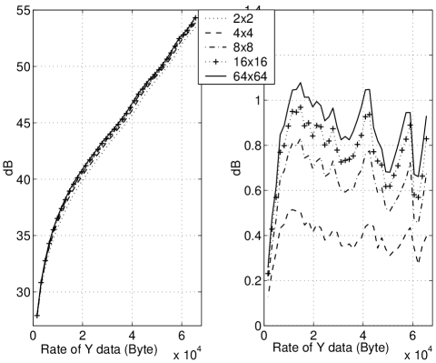
(a)                               (b)

Figure 10: (a) Coding performance comparison of Lenna image using different color format conversion methods. (b) Coding gain of the format conversion using larger blocks against the format conversion with 2 by 2 blocks. Luminance data are coded by using SPIHT with shape adaptive DWT (SA-DWT) after rotation transform and the PSNR is calculated with $Y$ and $\hat{Y}$ in Fig. 5 .

The coding performance of the format conversion with different block sizes is shown in Fig. 10. Since the interpolated data at boundary pixels of each block is less smooth, the interpolation method with a smaller number of boundary pixels can give a better result. For example, 75% of Y data are on block boundaries when 4 by 4 blocks are used whereas 12.3% are on block boundaries when 64 by 64 blocks are used. Therefore as shown in Fig. 10, the format conversion with larger blocks gives better results than that with smaller blocks although the complexity of decoding is higher.

IV-B Nonlinear transform with cropping

(a)                               (b)

Figure 11: Luminance PSNR difference between the rotation and horizontal shift methods after compression by using (a) JPEG and (b) SPIHT. 2 by 2 block format conversion is used in both cases.

The performance of horizontal shift and rotation methods after coding is shown in Fig. 11. Since, in JPEG coding (shown in (a)), high frequency components introduce more errors due to larger quantization step sizes chosen for them, the horizontal shift method, which introduces more high frequency components, results in worse performance. Also in JPEG coding, an image is efficiently coded by using EOB, so that increased high frequency energy translates into more bits, as the EOB happens later on average in a zigzag scan. Thus, as we expected, the horizontal shift transform generates more high frequency components and gives a worse result. But for the “Baboon” image, the image itself contains large high frequency components and most coefficients cannot be coded as EOB, therefore the high frequency components induced by the shift method have less of an impact than for other images. In this case, the added redundancy coming from the data shape of the rotation method may lead to worse performance than the horizontal shifting, given that the effect of additional high frequencies is not as significant for these images.

Contrary to JPEG coding, SPIHT coding does not compress high frequency components with larger quantization values. Instead it uses bit-plane encoding at all frequencies and the number of bit-planes transmitted at a given bit-rate is roughly the same at all frequencies. Therefore the coding performance of the shift method is comparable to that of the rotation method. But if the source is simple (i.e., not having large energy in high frequency bands) then the shift method provides worse energy compaction and so the result is worse (as shown in the case of “Lenna” image).

Figs. 11 (a) and (b) show that the coding gain of the rotation method is decreased as the bit-rate is increased, except when the bit-rate is less than 10KB. In the low bit-rate region, small coefficients are quantized to zero, therefore most coefficients are not transmitted because an EOB has been reached (in JPEG coding) or only a small number of coefficients is coded (in SPIHT coding). But in the shift method, many coefficients are large and cannot be quantized to zero. Therefore higher coding gain is achieved with the rotation method. As quantization values become smaller, the coefficients of the rotation method (which are quantized to zero in a low bit-rate region) are no longer quantized to zero and the bit-rate increases sharply. Instead, most coefficients of the shift method are already non-zero (in the low bit-rate region) and the bit-rate is increased more slowly. Therefore the coding gain of the rotation method is reduced as the bit-rate becomes higher.

IV-C Overall performance

As shown in Figs. 12 (a),(c) and (e), the IAD algorithms achieve better luminance PSNR except for low bit-rates, depending on format conversion and compression methods. With JPEG compression, the PSNR of the shift method drops sharply and the performance of this method is worse than that of CAI methods in case that the bit-rate is approximately under 50KB (i.e., the compression ratio is roughly $15:1$) whereas the rotation methods outperform the CAI method under all other compression ratios used in [27]. With SPIHT compression, the performance of shift and rotation with 2 by 2 block format conversion methods is similar (see Fig. 11 (b)) and they outperform the CAI method when the bit-rate is over 20KB or 25KB (i.e., a compression ratio is $39:1$ or $31:1$) as shown in Fig. 13. As expected, the rotation with 64 by 64 block transform method gives a better result than other proposed methods. Under same bit-rate, IAD algorithms can assign more bits for each pixel since the IAD algorithms only use approximately half of luminance data. This is the reason why the IAD methods outperform the CAI method. Also, as shown in our analysis (see Fig. 4), IAD algorithms outperform in a wider range of PSNR with the “Baboon” image (low spatial correlation) than with the “Lenna” and “Macaw” images (high spatial correlation).

In the chrominance data cases as in Figs. 12 (b), (d) and (f), the PSNR gain is even higher (though PSNR is not so meaningful in color components). In the CAI algorithm, if the 4:2:2 format is used for JPEG compression then two adjacent pixels use same color data and some color information is lost. But in the IAD algorithm, color format conversion is reversible and all color information can be presented. Although, even in the CAI method, there is no color information loss if JPEG with 4:4:4 format is used, the bit-rate for the color information is increased and so, by using this increased bit-rate, lower compression ratio can be applied in the IAD algorithm. In our experiments, chrominance data compression with 4:4:4 format is tested with SPIHT compression. Since the size of chrominance data of the CAI algorithm is 4 times larger than that of proposed ones, the bit budget per pixel of IAD algorithms is 4 times larger than that of conventional one and this gives a large PSNR gain.

Although shift and rotation with 2 by 2 block transform provide exactly the same chrominance data (since both transforms use the same 2 by 2 color format conversion), the chrominance PSNRs of the two algorithms are not identical. This shows that the luminance distortion also affects the quality of chrominance data.

In order to compare the error in a perceptually uniform color space, average $\Delta{E}$ in the CIELAB space is used for a second measure. As shown in Fig. 14, IAD methods (rotation with 64 by 64 block transform) provide smaller errors than CAI methods with both JPEG (under all compression ratios considered) and SPIHT (up to more than $50:1$).

In addition to the higher PSNR gain, lower average $\Delta{E}$ and lower complexity, the IAD algorithms have other advantages such as lower blocking artifacts after JPEG coding and fast consecutive capturing. Reduction of blocking artifacts is achieved because a lower compression ratio is used at a given rate. Additionally, because interpolation is done after decompression, it can reduce blocking artifacts similar to a de-blocking processing after JPEG decompression. Moreover luminance data and chrominance data use different block shapes, which may also help to reduce blocking artifacts. Figs. 18 (b) and (c) shows the result of CAI and IAD methods, respectively. As expected, the result of the CAI method shows more blocking artifacts. Finally, fast consecutive capturing is possible since the compression time is shorter because only around half of Y data has to be encoded, while interpolation (in case of 2 by 2 format conversion) and post processing functions are not needed during the capture process.

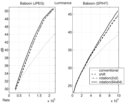
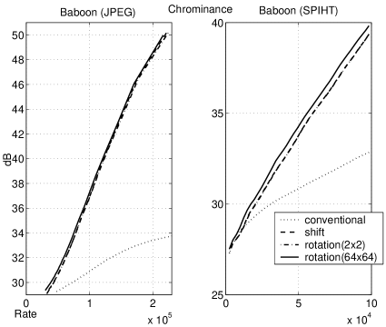
(a)	(b)
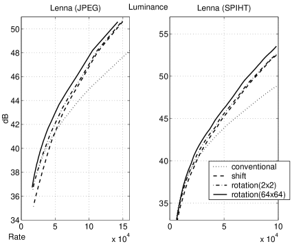
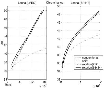
(c)	(d)
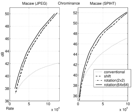
(e)	(f)

Figure 12: The curves indicate the luminance and chrominance PSNR after applying overall coding schemes. shift and rotation (2x2 and 64x64) indicate non-linear transform used in the IAD method and conventional indicates the CAI method.

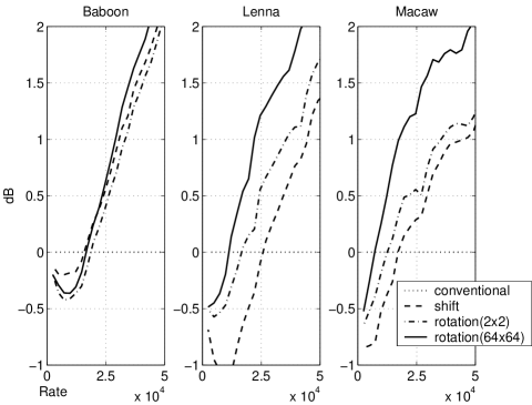
Figure 13: The PSNR gain of different proposed methods against the conventional method. Vertical and horizontal axes indicate the luminance PSNR gain and overall bit-rate respectively and SPIHT is used as a compression method.

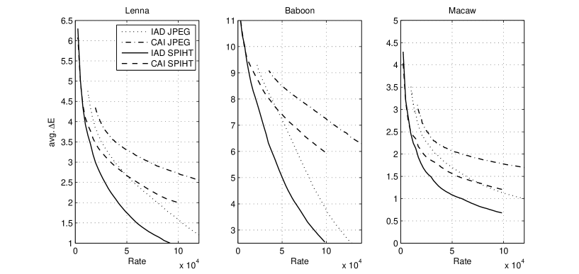
Figure 14: The curves indicate the average $\Delta{E}$ of IAD and CAI methods with bilinear interpolation.

V Comparison with adaptive interpolation

In the proposed methods, interpolation is done after decompression, so more complex interpolation can be applied without increasing the complexity of the encoding system. Therefore, with lower complexity than that of bilinear interpolation, we can achieve visually better results. Since coding errors can give negative effects to the performance of interpolation, in this chapter, we compare the performance of proposed methods with more complex interpolation methods.

From the compression viewpoint, bilinear interpolation is a good method because it results in smoother (and thus easier to compress) images. Also in the IAD algorithms, the color components generated by using the bilinear interpolation have an error that results from averaging the error of neighbor pixels, so that the average distortion of interpolated color components can be lower than that of coded color components (similar to the 1-D case shown in (9)). This is also confirmed by the experimental results shown in Fig. 10 (a) and Fig. 12 (c) (SPIHT). Note that the two figures have different horizontal axis and the rate used in Fig. 12 is 1.5 times larger than that of Fig. 10. The result verifies that PSNR is increased after interpolation except at high bit-rates (where round-off error plays an important role because the coding errors are relatively small).

Although bilinear interpolation is simple and fast, it works like a low pass filtering and does produce smoothing of edges. To preserve more edge information, several different adaptive interpolation algorithms have been proposed [28]. Depending on the local information, adaptive interpolation algorithms take a different interpolation method and use the correlation of different color components. After applying the adaptive interpolation, the interpolated image has more edge information (i.e., more high frequency components) and it cannot be easily compressed. In this sense the IAD algorithms have an advantage. Note that the IAD algorithms perform interpolation after decoding, so the coded data is independent of interpolation algorithms. But due to lossy compression, IAD and CAI algorithms have different data before the interpolation. Therefore it could happen that they have different edge information and take a different directional interpolation method for pixels at the same position. This results in high distortion in the generated color components. Also, the error of one color component is involved in the interpolation of other color components and the distortion of generated pixels can be increased. As a result, by using the adaptive interpolation, the IAD algorithms achieve some gains from data smoothness before compression (especially in the case of rotation with 64 by 64 block format conversion) but may lose in performance from choosing different directions during interpolation due to distorted data. Therefore when error-sensitive interpolation methods (which are very sensitive about the quantization noise of existing compression methods) are required, interpolation aware compression methods (which can keep more information used in the interpolation) are needed. But in this paper, we mainly focus on the performance comparison between IAD and CAI algorithms, and we use existing compression methods with minor modification.

To verify the performance of the IAD algorithms with the adaptive interpolation, we consider 3 different adaptive interpolation algorithms, namely, constant hue-based, gradient based and median-based interpolation [4].

Constant hue-based interpolation is proposed by Cok [29] and Kimmel [8], where hue is defined by a vector of ratios as ($R/G,~{}B/G$). In this algorithm, the green color component is used as a denominator and a small error of the green component may induce a large error in hue, especially when green values are small. Therefore the IAD algorithms do not provide good performance when this interpolation is applied.

Gradient based interpolation is proposed by Laroche and Prescott [30]. In this algorithm, at first, green components on blue (red) pixel positions are determined by using directional bilinear interpolation, where the direction is selected by the gradient of neighboring blue (red) components. After determining green components, blue (red) components are interpolated from the differences between blue (red) and green components. Fig. 15 shows the coding results of IAD algorithms. With JPEG compression, the performance of IAD algorithms (except rotation with 64 by 64 block format conversion) is worse than that of the CAI algorithm since different direction is determined by large error in high frequency components and blocking effect and the error of green components also affects red and blue components. But with SPIHT compression, the coding error is evenly distributed and different directional interpolation is reduced. Therefore as shown in Fig. 15 (d), the IAD algorithms outperform the CAI algorithm although the gain is smaller than when bilinear interpolation is used (shown in Fig. 13).

The performance is also tested with Median-based interpolation (proposed by Freeman [31]) which employs two step processes. The first pass is the bilinear interpolation and the second pass is selecting the median of color differences of neighboring pixels. Fig. 16 shows the coding results of IAD algorithms with a 3 by 3 median filter. Similar to the gradient-based interpolation, the IAD algorithms provide worse results when JPEG is applied. But with SPIHT, IAD algorithms still provide better results up to $20:1$ or $40:1$ compression ratio depending on the format conversion methods. Fig. 17 shows average $\Delta{E}$ in the CIELAB space. IAD algorithms provide better results up to more than $20:1$ compression ratio and then the average $\Delta{E}$ of both algorithm goes similar. Fig. 19 shows the results after applying bilinear and Freeman interpolation. As expected, The image with Freeman interpolation (Fig. 19 (c)) is sharper and close to the original image (Fig. 18 (a)).

As a result, the IAD algorithms with SPIHT provide better results with the gradient based and median-based interpolation. But due to coding inefficiency, irregular coding error and blocking effect, adaptive interpolation for a given pixel may be different depending on using quantized or unquantized data, resulting in potential degradation after interpolation when quantized data is used interpolation for each pixel. Therefore the performance of the IAD algorithms with JPEG is worse.

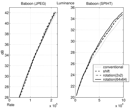
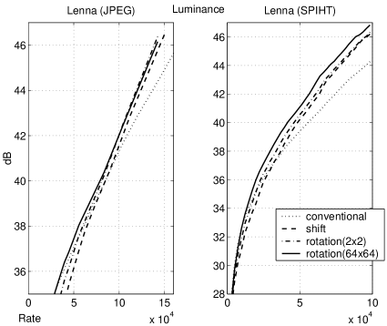
(a)	(b)
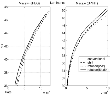
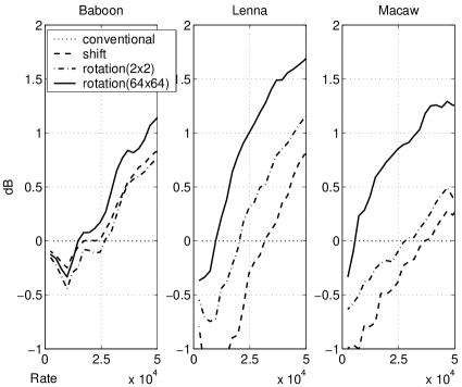
(c)	(d)

Figure 15: The curves in (a), (b) and (c) indicate the luminance PSNR after applying overall coding schemes with gradient based interpolation. The curve in (d) indicates the PSNR gain of different IAD methods against the CAI method with SPIHT.

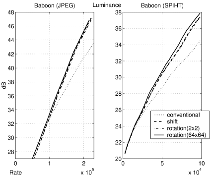
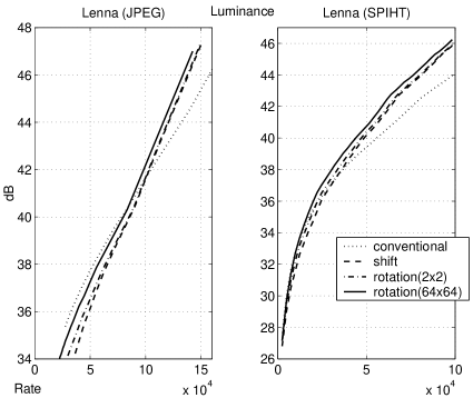
(a)	(b)
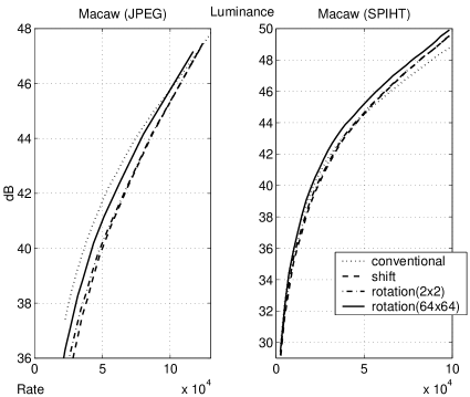
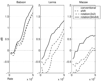
(c)	(d)

Figure 16: The curves in (a), (b) and (c) indicate the luminance PSNR after applying overall coding schemes with median-based interpolation and SPIHT. The curve in (d) indicates the PSNR gain of different IAD methods against the CAI method with SPIHT.

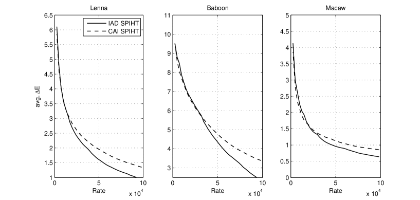
Figure 17: The curves indicate the average $\Delta{E}$ of IAD and CAI methods with median-based interpolation and SPIHT.

VI CONCLUSION

In this paper, we investigated the redundancy decreasing method that merges an image processing stage and an image compression stage. Several color format conversion algorithms and shift and rotation transforms are introduced to compress CFA images before making full color images by interpolation. We showed that the proposed algorithms outperform the conventional method in the full range of compression ratios for JPEG coding with bilinear interpolation and up to $20:1$ or $40:1$ compression ratio (depending on the color format conversion and interpolation methods) for SPIHT coding when the bilinear, gradient based and median-based interpolation are applied. Also we analyzed the PSNR gain and explained why it becomes higher as the compression ratio becomes lower, showing also a 1D DPCM sequence example to provide some intuition. Because the proposed algorithms use only around half the amount of Y data and only need an additional simple transform, the computational complexity can be decreased. Also adaptive interpolation methods can be applied without increasing the encoder complexity, so fast consecutive capturing can be achieved with visually better results.

In this paper, we tried to minimize the changes to existing compression methods in order to focus on the performance of changing the encoding order (i.e., the order of interpolation and compression). The performance of the IAD method can be improved with different entropy coding (in SPIHT). Also, in the rotation method, a new quantization table may be useful for a JPEG codec, due to the directional difference of human visual sensitivity.

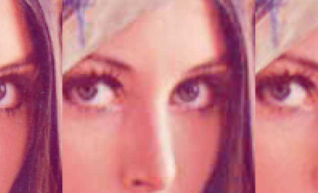
(a)                                            (b)                                            (c)

Figure 18: Comparison of blocking artifacts. (a) is the original image, and (b) and (c) are the images after applying CAI and IAD, respectively. Bilinear interpolation and JPEG compression are used, where the compression ratio is $35.2:1$.

(a)                                            (b)                                            (c)

Figure 19: Comparison of different interpolation. (a) and (b) are the images after applying CAI and IAD, respectively. Bilinear interpolation and SPIHT compression are used. (c) is the images after applying CAI with Freeman interpolation. Compression ratio used is $16:1$. Note that the encoding of (b) and (c) are identical.

References

- [1] W. Pennebaker and J. Mitchell, JPEG Still Image Data Compression Standard. Van Nostrand Reinhold, 1994.
- [2] T. Yamada, K. Ikeda, Y. Kim, H. Wakoh, T. Sakamoto, K. Ogawa, E. Okamoto, K. Masukane, K. Oda, and M. Inuiya, “A progressive scan CCD image sensor for dsc application,” IEEE Trans. on Solid-State Circuits, pp. 2044–2054, Dec. 2000.
- [3] S. Yamanaka, “Solid state camera,” U.S. Patent 4,054,906, 1977.
- [4] R. Ramanath, W. E. Snyder, and G. L. Bilbro, “Demosaicking methods for Bayer color arrays,” Journal of Electronic Imaging, vol. 11(3), pp. 306–315, July 2002.
- [5] P. Longère, X. Zhang, P. B. Delahunt, and D. H. Brainard, “Perceptual assessment of demosaicing algorithm performance,” Procedings of the IEEE, vol. 90, pp. 123–132, Jan. 2002.
- [6] H. J. Trussell and R. E. Hartwig, “Mathematics for demosaicking,” IEEE Trans. on Image Processing, vol. 11, pp. 485–492, Apr. 2002.
- [7] J. Adams, “Design of practical color filter array interpolation algorithms for digital cameras .2,” in Proc. Int. Conf. on Image Proc., vol. 1, 1998, pp. 488–492.
- [8] R. Kimmel, “Demosaicing: Image reconstruction from color CCD samples,” IEEE Trans. on Image Processing, vol. 4, pp. 725–733, June 1995.
- [9] N. Kehtarnavaz, H. J. Oh, and Y. Yoo, “Color filter array interpolation using color correlation and directional derivatives,” Journal of Electronic Imaging, vol. 12, pp. 621–632, Oct. 2003.
- [10] C. Herley, “A post-processing algorithm for compressed digital camera images,” in Proc. Int. Conf. on Image Proc., vol. 1, 1998, pp. 396–400.
- [11] Z. Baharav and R. Kakarala, “Compression aware demosaicing methods,” in Proc. SPIE, vol. 4667, 2002, pp. 149–156.
- [12] C. C. Koh and S. K. Mitra, “Compression of Bayer color filter array data,” in Proc. Int. Conf. on Image Proc., Oct. 2003, pp. 255–258.
- [13] S.-Y. Lee and A. Ortega, “A novel approach of image compression in digital cameras with a Bayer color filter array,” in Proc. Int. Conf. on Image Proc., vol. 3, 2001, pp. 482–485.
- [14] J. Shapiro, “Embedded image coding using zerotrees of wavelet coefficients,” IEEE Trans. on Signal Processing, vol. 41, pp. 3445–3462, Dec. 1993.
- [15] A. Said and W. Pearlman, “A new, fast and efficient image codec based on set partitioning,” IEEE Trans. on Circuits and Systems for Video Tech., vol. 6, pp. 243–250, June 1996.
- [16] D. Taubman, “High performance scalable image compression with EBCOT,” IEEE Trans. on Image Processing, vol. 9, pp. 1158–1170, July 2000.
- [17] D. S. Taubman and M. W. Marcellin, JPEG2000 Image Compression Fundamentals, Standards and Practice. Kluwer Academic Publisher, 2002.
- [18] T. Cover and J. Thomas, Elements of Information Theory. John Wiley & Sons, 1991.
- [19] E. Hamilton. (1992) JPEG file interchange format. [Online]. Available: http://www.w3.org/Graphics/JPEG/jfif3.pdf
- [20] A. Kaup, “Object-based texture coding of moving video in MPEG-4,” IEEE Trans. on Circuits and Systems for Video Tech., vol. 9, pp. 5–15, Feb. 1999.
- [21] T. Sikora, “Low complexity shape-adaptive DCT for coding of arbitrarily shaped image segments,” Signal Processing: Image Communication, vol. 7, pp. 381–395, 1995.
- [22] R. Stasidski and J. Konrad, “New class of fast shape-adaptive orthogonal transforms and their application to region-based image compression,” IEEE Trans. on Circuits and Systems for Video Tech., vol. 9, pp. 16–34, Feb. 1999.
- [23] S. Li and W. Li, “Shape-adaptive discrete wavelet transforms for arbitrarily shaped visual object coding,” IEEE Trans. on Circuits and Systems for Video Tech., vol. 10, pp. 725–743, Aug. 2000.
- [24] S.-Y. Lee and A. Ortega. (2004) Experimental results of IAD and CAI methods for performance comparison. [Online]. Available: http://sipi.usc.edu/ortega/Sangyong
- [25] HP. Hp photosmart digital camera - image handling: bpy0038. [Online]. Available: http://h10025.www1.hp.com
- [26] KODAK. (2005) Digital camera FAQs. [Online]. Available: http://faqs.kodak.com/Digital_Cameras_English/TFAQ3.shtm
- [27] I. J. Group, “IJG’s jpeg software release 6a,” Feb. 1996.
- [28] B. K. Gunturk, J. Glotzbach, Y. Altunbasak, R. W. Schafer, and R. M. Mersereau, “Demosaicking: Color filter array interpolation,” IEEE Signal Processing Magazine, vol. 22, pp. 44–54, Jan. 2005.
- [29] D. R. Cok, “Signal processing method and apparatus for producing interpolated chrominance values in a sampled color image signal,” U.S. Patent 4,642,678, 1987.
- [30] C. A. Laroche and M. A. Prescott, “Apparatus and method for adaptively interpolating a full color image utilizing chrominance gradients,” U.S. Patent 5,373,322, 1994.
- [31] T. Freeman, “Median filter for reconstructing missing color samples,” U.S. Patent 4,724,395, 1988.