Manipulating Scrip Systems: Sybils and Collusion

Abstract

Game-theoretic analyses of distributed and peer-to-peer systems typically use the Nash equilibrium solution concept, but this explicitly excludes the possibility of strategic behavior involving more than one agent. We examine the effects of two types of strategic behavior involving more than one agent, sybils and collusion, in the context of scrip systems where agents provide each other with service in exchange for scrip. Sybils make an agent more likely to be chosen to provide service, which generally makes it harder for agents without sybils to earn money and decreases social welfare. Surprisingly, in certain circumstances it is possible for sybils to make all agents better off. While collusion is generally bad, in the context of scrip systems it actually tends to make all agents better off, not merely those who collude. These results also provide insight into the effects of allowing agents to advertise and loan money. While many extensions of Nash equilibrium have been proposed that address collusion and other issues relevant to distributed and peer-to-peer systems, our results show that none of them adequately address the issues raised by sybils and collusion in scrip systems.

1 Introduction

Studies of filesharing networks have shown that more than half of participants share no files adar00 ; Hughes05 . Creating a currency with which users can get paid for the service they provide gives users an incentive to contribute. Not surprisingly, scrip systems have often been proposed to prevent such free-riding, as well as to address resource-allocation problems more broadly. For example, KARMA used scrip to prevent free riding in P2P networks karma03 and Mirage mirage and Egg egg use scrip to allocate resources in a wireless sensor network testbed and a grid respectively

Chun et al. ng05 studied user behavior in a deployed scrip system and observed that users tried various (rational) manipulations of the auction mechanism used by the system. Their observations suggest that system designers will have to deal with game-theoretic concerns. Game-theoretic analyses of scrip systems (e.g., johari06 ; scrip06 ; hens ; scrip07 ) have focused on Nash equilibrium. However, because Nash equilibrium explicitly excludes strategic behavior involving more than one agent, it cannot deal with many of the concerns of systems designers. One obvious concern is collusion among sets of agents, but there are more subtle concerns. In a P2P network, it is typically easy for an agent to join the system under a number of different identities, and then mount what has been called a sybil attack sybil . While these concerns are by now well understood, their impact on a Nash equilibrium is not, although there has been some work on the effects of multiple identities in auctions yokoo04 . In this paper we examine the effects of sybils and collusion on scrip systems. We show that if such strategic behavior is not taken into account, the performance of the system can be significantly degraded; indeed the scrip system can fail in such a way that all agents even stop providing service entirely. Perhaps more surprisingly, there are circumstances where sybils and collusion can improve social welfare. Understanding the circumstances that lead to these different outcomes is essential to the design of stable and efficient scrip systems.

In scrip systems where each new user is given an initial amount of scrip, there is an obvious benefit to creating sybils. Even if this incentive is removed, sybils are still useful: they can be used to increase the likelihood that an agent will be asked to provide service, which makes it easier for him to earn money. This means that, in equilibrium, those agents who have sybils will tend to spend less time without money and those who do not will tend to spend more time without money, relative to the distribution of money if no one had sybils. This increases the utility of sybilling agents at the expense of non-sybilling agents. The overall effect is such that, if a large fraction of the agents have sybils (even if each has only a few), agents without sybils typically will do poorly. From the perspective of an agent considering creating sybils, the first few sybils can provide him with a significant benefit, but the benefits of additional sybils rapidly diminish. So if a designer can make sybilling moderately costly, the number of sybils actually created by rational agents will usually be relatively small.

If a small fraction of agents have sybils, the situation is more subtle. Agents with sybils still do better than those without, but the situation is not zero-sum. In particular, changes in the distribution of money can actually lead to a greater total number of opportunities to earn money. This, in turn, can result in an increase in social welfare: everyone is better off. However, exploiting this fact is generally not desirable. The same process that leads to an improvement in social welfare can also lead to a crash of the system, where all agents stop providing service. The system designer can achieve the same effects by increasing the average amount of money or biasing the volunteer selection process, so exploiting the possibility of sybils is generally not desirable.

Sybils create their effects by increasing the likelihood that an agent will be asked to provide service; our analysis of them does not depend on why this increase occurs. Thus, our analysis also applies to other factors that increase demand for an agent’s services, such as advertising. In particular, our results suggest that there are tradeoffs involved in allowing advertising. For example, many systems allow agents to announce their connection speed and other similar factors. If this biases requests towards agents with high connection speeds even when agents with lower connection speeds are perfectly capable of satisfying a particular request, then agents with low connection speeds will have a significantly worse experience in the system. This also means that such agents will have a strong incentive to lie about their connection speed.

While collusion in generally a bad thing, in the context of scrip systems with fixed prices, it is almost entirely positive. Without collusion, if a user runs out of money he is unable to request service until he is able to earn some. However, a colluding group can pool there money so that all members can make a request whenever the group as a whole has some money. This increases welfare for the agents who collude because agents who have no money receive no service.

Furthermore, collusion tends to benefit the non-colluding agents as well. Since colluding agents work less often, it is easier for everyone to earn money, which ends up making everyone better off. However, as with sybils, collusion does have the potential of crashing the system if the average amount of money is high.

While a designer should generally encourage collusion, we would expect that in most systems there will be relatively little collusion and what collusion exists will involve small numbers of agents. After all, scrip systems exist to try and resolve resource-allocation problems where agents are competing with each other. If they could collude to optimally allocate resources within the group, they would not need a scrip system in the first place. However, many of the benefits of collusion come from agents being allowed to effectively have a negative amount of money (by borrowing from their collusive partners). These benefits could also be realized if agents are allowed to borrow money, so designing a loan mechanism could be an important improvement for a scrip system. Of course, implementing such a loan mechanism in a way that prevents abuse requires a careful design.

These results about sybils and collusion indicate their role in scrip systems and in distributed and peer-to-peer systems more broadly is poorly addressed by existing solution concepts. We conclude by discussing some of the open questions they raise.

2 Model

Our model of a scrip system is essentially that of scrip07 . There are $n$ agents in the system. One agent can request a service which another agent can volunteer to fulfill. When a service is performed by agent $j$ for agent $i$, agent $i$ derives some utility from having that service performed, while agent $j$ loses some utility for performing it. The amount of utility gained by having a service performed and the amount lost by performing it may depend on the agent. We assume that agents have a type $t$ drawn from some finite set $T$ of types. We can describe the entire system using the tuple $(T,\vec{f},n,m)$, where $f_{t}$ is the fraction with type $t$, $n$ is the total number of agents, and $m$ is the average amount of money per agent. In this paper, we consider only standard agents, whose type we can characterize by a tuple $t=(\alpha_{t},\beta_{t},\gamma_{t},\delta_{t},\rho_{t},\chi_{t})$, where

• $\alpha_{t}$ reflects the cost of satisfying a request;

• $\beta_{t}$ is the probability that the agent can satisfy a request

• $\gamma_{t}$ measures the utility an agent gains for having a request satisfied;

• $\delta_{t}$ is the rate at which the agents discounts utility (so a unit of utility in $k$ steps is worth only $\delta^{k/n}_{t}$ as much as a unit of utility now)—intuitively, $\delta_{t}$ is a measure of an agent’s patience (the larger $\delta_{t}$ the more patient an agent is, since a unit of utility tomorrow is worth almost as much as a unit today);

• $\rho_{t}$ represents the (relative) request rate (since not all agents make requests at the same rate)—intuitively, $\rho_{t}$ characterizes an agent’s need for service; and

• $\chi_{t}$ represents the relative likelihood of being chosen to satisfy a request. This might be because, for example, agents with better connection speeds are preferred.

The parameter $\chi_{t}$ did not appear in scrip07 ; otherwise the definition of a type is identical to that of scrip07 .

We model the system as running for an infinite number of rounds. In each round, an agent is picked with probability proportional to $\rho_{t}$ to request service: a particular agent of type $t$ is chosen with probability $\rho_{t}/\sum_{t^{\prime}}f_{t^{\prime}}n\rho_{t^{\prime}}$. Receiving service costs some amount of scrip that we normalize to $1. If the chosen agent does not have enough scrip, nothing will happen in this round. Otherwise, each agent of type $t$ is able to satisfy this request with probability $\beta_{t}$, independent of previous behavior. If at least one agent is able and willing to satisfy the request, and the requester has type $t^{\prime}$, then the requester gets a benefit of $\gamma_{t^{\prime}}$ utils (the job is done) and one of the volunteers is chosen at random (weighted by the $\chi_{t}$) to fulfill the request. If the chosen volunteer has type $t$, then that agent loses $\alpha_{t}$ utils, and receives a dollar as payment. The utility of all other agents is unchanged in that round. The total utility of an agent is the discounted sum of the agent’s round utilities. To model the fact that requests will happen more frequently the more agents there are, we assume that the time between rounds is $1/n$. This captures the intuition that things are really happening in parallel and that adding more agents should not change an agent’s request rate.

In our previous work scrip06 ; scrip07 , we proved a number of results about this model:

• There is an ($\epsilon$-) Nash equilibrium where each agent chooses a threshold $k$ and volunteers to work only when he has less than $k$ dollars. For this equilibrium, an agent needs no knowledge about other agents, as long as he knows how often he will make a request and how often he will be chosen to work (both of which he can determine empirically).

• Social welfare is essentially proportional to the average number of agents who have money, which in turn is determined by the types of agents and the average amount of money the agents in the system have.

• Social welfare increases as the average amount of money increases, up to a certain point. Beyond that point, the system “crashes”: the only equilibrium is the trivial equilibrium where all agents have threshold 0.

Our proofs of these results relied on the assumption that all types of agents shared common values of $\beta$, $\chi$, and $\rho$. To model sybils and collusion, we need to remove this assumption. The purpose of the assumption was to make each agent equally likely to be chosen at each step, which allows entropy to be used to determine the likelihood of various outcomes, just as in statistical mechanics jaynes . When the underlying distribution is no longer uniform, entropy is no longer sufficient to analyze the situation, but, as we show here, relative entropy cover (which can be viewed as a generalization of entropy to allow non-uniform underlying distributions) can be used instead. The essential connection is that where entropy can be interpreted as a measure of the number of ways a distribution can be realized, relative entropy can be interpreted as a weighted measure where some outcomes are more likely to be seen than others. While this connection is well understood and has been used to derive similar results for independent random variables csiszar84 , we believe that our application of the technique to a situation where the underlying random variables are not independent is novel and perhaps of independent interest. Using relative entropy, all our previous results can be extended to the general case. The details of this extension are in the appendix.

This model does make a number of simplifying assumptions, but many can be relaxed without changing the fundamental behavior of the system (albeit at the cost of greater strategic and analytic complexity). For example, rather than all requests having the same value $\gamma$, the value of a request might be stochastic. This would mean that an agent may forgo a low-valued request if he is low on money. This fact may impact the threshold he chooses and introduces new decisions about which requests to make, but the overall behavior of the system will be essentially unchanged.

A more significant assumption is that prices are fixed. However, our results provide insight even if we relax this assumption. With variable prices, the behavior of the system depends on the value of $\beta$. For large $\beta$, where there are a significant number of volunteers to satisfy most requests, we expect the resulting competition to effectively produce a fixed price, so our analysis applies directly. For small $\beta$, where there are few volunteers for each request, variable prices can have a significant impact. In particular, sybils and collusion are more likely to result in inflation or deflation rather than a change in utility.

However, allowing prices to be set endogenously, by bidding, has a number of negative consequences. For one thing, it removes the ability of the system designer to optimize the system using monetary policy. In addition, for small $\beta$, it makes it possible for colluding agents to form a cartel to fix prices on a resource they control. It also greatly increases the strategic complexity of using the system: rather than choosing a single threshold, agents need an entire pricing scheme. Finally, the search costs and costs of executing a transaction are likely to be higher with variable prices. Thus, in many cases we believe that adopting a fixed price or a small set of fixed prices is a reasonable design decision.

3 Sybils

Unless identities in a system are tied to a real world identity (for example by a credit card), it is effectively impossible to prevent a single agent from having multiple identities sybil . Nevertheless, there are a number of techniques that can make it relatively costly for an agent to do so. For example, Credence uses cryptographic puzzles to impose a cost each time a new identity wishes to join the system credence . Given that a designer can impose moderate costs to sybilling, how much more need she worry about the problem? In this section, we show that the gains from creating sybils when others do not diminish rapidly, so modest costs may well be sufficient to deter sybilling by typical users. However, sybilling is a self-reinforcing phenomenon. As the number of agents with sybils gets larger, the cost to being a non-sybilling agent increases and so the incentive to create sybils becomes stronger. Therefore measures to discourage or prevent sybilling should be taken early before this reinforcing trend can start. Finally, we examine the behavior of systems where only a small fraction of agents have sybils. We show that under these circumstances a wide variety of outcomes are possible (even when all agents are of a single type), ranging from a crash (where no service is provided) to an increase in social welfare. This analysis provides insight into the tradeoffs between efficiency and stability that occur when controlling the money supply of the system’s economy.

When an agent of type $t$ creates sybils, he does not change anything about himself but rather how other agents percieve him. Thus the only change to his type might be an increase in $\chi_{t}$ if sybils cause other agents to choose him more often. We assume that each sybil is as likely to be chosen as the original agent, so creating $s$ sybils increases $\chi_{t}$ by $s\chi_{t}$. (Sybils may have other impacts on the system, such as increased search costs, but we expect these to be minor.) The amount of benefit he derives from this depends on two probabilities: $p_{e}$ (the probability he will earn a dollar this round if he volunteers) and $p_{s}$ (the probability he will be chosen to spend a dollar and there is another agent willing and able to satisfy his request). When $p_{e}<p_{s}$, the agent has more opportunities to spend money than to earn money, so he will regularly have requests go unsatisfied due to a lack of money. In this case, the fraction of requests he has satisfied is roughly $p_{e}/p_{s}$, so increasing $p_{e}$ results in a roughly linear increase in utility. When $p_{e}$ is close to $p_{s}$, the increase in satisfied requests is no longer linear, so the benefit of increasing $p_{e}$ begins to diminish. Finally, when $p_{e}>p_{s}$, most of the agent’s requests are being satisfied so the benefit from increasing $p_{e}$ is very small. Figure 2 illustrates an agent’s utility as $p_{e}$ varies for $p_{s}=.0001$. We formalize the relationship between $p_{e}$, $p_{s}$, and utility in the following theorem.

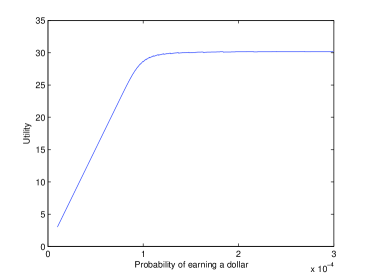
Figure 1: The effect of $p_{e}$ on utility

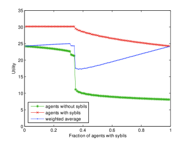
Figure 2: The effect of sybils on utility

Theorem 3.1

Let $p_{s}$ be the probability that a particular agent is chosen to make a request in a given round and there is some other agent willing and able to satisfy it, $p_{e}$ be the probability that the agent earns a dollar given that he volunteers, $r=p_{e}/p_{s}$, and $k$ be the agent’s strategy (i.e., threshold). In the limit as the number of rounds goes to infinity, the fraction of the agent’s requests that have an agent willing and able to satisfy them that get satisfied is $(r-r^{k+1})/(1-r^{k+1})$ if $r\neq 1$ and $k/(k+1)$ if $r=1$.

Proof

Since we consider only requests that have another agent willing and able to satisfy them, the request is satisfied whenever the agent has a non-zero amount of money. Since we have a fixed strategy and probabilities, consider the Markov chain whose states are the amount of money the agent has and the transitions describe the probability of the agent changing from one amount of money to another. This Markov chain satisfies the requirements to have a stationary distribution and it can be easily verified that the distribution gives the agent probability $r^{i}(1-r)/(1-r^{k+1})$ of having $i$ dollars if $r\neq 1$ and probability $1/(k+1$) if $r=1$ cover . This gives the probabilities given in the theorem.

Theorem 3.1 also gives insight into the equilibrium behavior with sybils. Clearly, if sybils have no cost, then creating as many as possible is a dominant strategy. However, in practice, we expect there is some modest overhead involved in creating and maintaining a sybil, and that a designer can take steps to increase this cost without unduly burdening agents. With such a cost, adding a sybil might be valuable if $p_{e}$ is much less than $p_{s}$, and a net loss otherwise. This makes sybils a self-reinforcing phenomenon. When a large number of agents create sybils, agents with no sybils have their $p_{e}$ significantly decreased. This makes them much worse off and makes sybils much more attractive to them. Figure 2 shows an example of this effect. This self-reinforcing quality means it is important to take steps to discourage the use of sybils before they become a problem. Luckily, Theorem 3.1 also suggests that a modest cost to create sybils will often be enough to prevent agents from creating them because with a well chosen value of $m$, few agents should have low values of $p_{e}$.

We have interpreted Figures 2 and 2 as being about changes in $\chi$ due to sybils, but the results hold regardless of what caused differences in $\chi$. For example, agents may choose a volunteer based on characteristics such as connection speed or latency. If these characteristics are difficult to verify and do impact decisions, our results show that agents have a strong incentive to lie about them. This also suggests that the decision about what sort of information the system should enable agents to share involves tradeoffs. If advertising legitimately allows agents to find better service or more services they may be interested in, then advertising can increase social welfare. But if these characteristics impact decisions but have little impact on the actual service, then allowing agents to advertise them can lead to a situation like that in Figure 2, where some agents have a significantly worse experience.

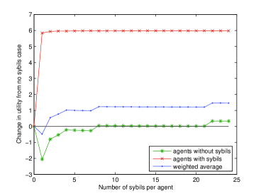
Figure 3: Sybils can improve utility

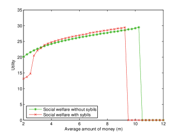
Figure 4: Sybils can cause a crash

We have seen that when a large fraction of agents have sybils, those agents without sybils tend to be starved of opportunities to work. However, as we saw in Figure 2, when a small fraction of agents have sybils this effect (and its corresponding cost) is small. Surprisingly, if there are few agents with sybils, an increase in the number of sybils these agents have can actually result in a decrease of their effect on the other agents. Because agents with sybils are more likely to be chosen to satisfy any particular request, they are able to use lower thresholds and reach those thresholds faster than they would without sybils, so fewer are competing to satisfy any given request. Furthermore, since agents with sybils can almost always pay to make a request, they can provide more opportunities for other agents to satisfy requests and earn money. Social welfare is essentially proportional to the number of satisfied requests (and is exactly proportional to it if everyone shares the same values of $\alpha$ and $\gamma$), so a small number of agents with a large number of sybils can improve social welfare, as Figure 4 shows. Note that this is not necessarily a Pareto improvement. For the choice of parameters in this example, social welfare increases when the agents create at least two sybils, but agents without sybils are worse off unless the agents with sybils create at least eight sybils. As the number of agents with sybils increases, they are forced to start competing with each other for opportunities to earn money and so are forced to adopt higher thresholds and this benefit disappears. This is what causes the discontinuity in Figure 2 when approximately a third of the agents have sybils.

This observation about the discontinuity also suggests another way to mitigate the negative effects of sybils: increase the amount of money in the system. This effect can be seen in Figure 4, where for $m=2$ social welfare is very low with sybils but by $m=4$ it is higher than it would be without sybils.

Unfortunately, increasing the average amount of money has its own problems. Recall from Section 2 that, if the average amount of money per agent is too high, the system will crash. It turns out that just a small number of agents creating sybils can have the same effect, as Figure 4 shows. With no sybils, the point at which social welfare stops increasing and the system crashes is between $m=10.25$ and $m=10.5$. If one fifth of the agents each create a single sybil, the system crashes if $m=9.5$, a point where, without sybils, the social welfare was near optimal. Thus, if the system designer tries to induce optimal behavior without taking sybils into account, the system will crash. Moreover, because of the possibility of a crash, raising $m$ to tolerate more sybils is effective only if $m$ was already set conservatively.

This example shows that there is a significant tradeoff between efficiency and stability. Setting the money supply high can increase social welfare, but at the price of making the system less stable. Moreover, as the following theorem shows, whatever efficiencies can be achieved with sybils can be achieved without them, at least if there is only one type of agent. The theorem does require a technical condition similar in spirit to $N$-replica economies mascolell to rule out transient equilibria that exist only for limited values of $n$. In our results, we are interested in systems $(T,\vec{f},n,m)$ where $T$, $\vec{f}$, and $m$ are fixed, but $n$ varies. This leads to a small technical problem: there are values of $n$ for which $\vec{f}$ cannot be the fraction of agents of each type nor can $m$ be the average amount of money (since, for example, $m$ must be a multiple of $1/n$). This technical concern can be remedied in a variety of ways; the approach we adopt is one used in the literature on $N$-replica economies

Definition 1

A strategy profile $\vec{k}$ is an asymptotic equilibrium for a system $(T,\vec{f},n,m)$ if for all $n^{\prime}$ such that $n^{\prime}=cn$ for integer $c>0$, $\vec{k}$ is a Nash equilibrium for $(T,\vec{f},n^{\prime},m)$. 

Consider a system where all agents have the same type $t$. Suppose that some subset of the agents have created sybils, and all the agents in the subset have created the same number of sybils. We can model this by simply taking the agents in the subsets to have a new type $s$, which is identical to $t$ except that the value of $\chi$ increases. Thus, we state our results in terms of systems with two types of agents, $t$ and $s$.

Theorem 3.2

Suppose that $t$ and $s$ are two types that agree except for the value of $\chi$, and that $\chi_{t}<\chi_{s}$. If $(k_{t},k_{s})$ is an asymptotic equilibrium for $(\{t,s\},\vec{f},m)$ with social welfare $x$, then there exists an $m^{\prime}$ and $n^{\prime}$ such that $(k_{s})$ is an asymptotic equilibrium for $(\{t\},\{1\},n^{\prime},m^{\prime})$ with social welfare at least $x$.

Proof

We show this by finding an $m^{\prime}$ such that agents in the second system that play some strategy $k$ get essentially the same utility that an agent with sybils would by playing that strategy in the first system. Since $k_{s}$ was the optimal strategy for agents with sybils in the first system, it must be optimal in the second system as well. Since agents with sybils have greater utility than those without (they could always avoid volunteering some fraction of the time to effectively lower $\chi_{s}$), social welfare will be at least as high in the second system as in the first.

Once strategies are fixed, an agent’s utility depends only on $\alpha_{t}$, $\gamma_{t}$, $\delta_{t}$, $p_{s}$, and $p_{e}$. The first three are constants. Because the equilibrium is asymptotic, for sufficiently large $cn$, almost every request by an agent with money is satisfied (the expected number of agents wishing to volunteer is a constant fraction of $cn$). Therefore, $p_{s}$ is essentially $1/cn$, his probability of being chosen to make a request. With fixed strategies, any value of $p_{e}$ between 0 and $\beta_{t}$ can be achieved by taking the appropriate $m^{\prime}$. Take $m^{\prime}$ such that, if every agent in the second system plays $k_{s}$, the resulting $p_{e}$ will be the same as the agents with sybils had in the original equilibrium. Note that $p_{s}$ may decrease slightly because fewer agents will be willing to volunteer, but we can take $n^{\prime}=cn$ for sufficiently large $c$ to make this decrease arbitrarily small.

The analogous result for systems with more than one type of agent is not true. Consider the situation shown in Figure 2, where forty percent of the agents have two sybils. With this population, social welfare is lower than if no agents had sybils. However, the same population could be interpreted simply as having two different types, one of whom is naturally more likely to be chosen to satisfy a request. In this situation, if the agents less likely to be chosen created exactly two sybils each, the each agent would then be equally likely to be chosen and social welfare would increase. While changing $m$ can change the relative quality of the two situations, a careful analysis of the proof of Theorem 3.2 shows that, when each population is compared using its optimal value of $m$, social welfare is greater with sybils. While situations like this show that it is theoretically possible for sybils to increase social welfare beyond what is possible by adjusting the average amount of money, this outcome seems unlikely in practice. It relies on agents creating just the right number of sybils. For situations where such a precise use of sybils would lead to a significant increase in social welfare, a designer could instead improve social welfare by biasing the algorithm agents use for selecting which volunteer will satisfy the request.

4 Collusion

Agents that collude gain two major benefits. The primary benefit is that they can share money, which simultaneously makes them less likely to run out of money and be unable to make a request and allows them to pursue a joint strategy for determining when to work. The secondary benefit, but important in particular for larger collusive groups, is that they can satisfy each other’s requests. The effects of collusion on the rest of the system depend crucially on whether agents are able to volunteer to satisfy requests when they personally cannot satisfy the request but one of their colluding partners can. In a system where a request is for computation, it seems relatively straightforward for an agent to pass the computation to a partner to perform and then pass the answer back to the requester. On the other hand, if a request is a piece of a file it seems less plausible that an agent would accept a download from someone other than the person he expects and it seems wasteful to have the chosen volunteer download it for the sole purpose of immediately uploading it. If it is possible for colluders to pass off requests in this fashion, they are able to effectively act as sybils for each other, with all the consequences we discussed in Section 3. However, if agents can volunteer only for requests they can personally satisfy, the effects of collusion are almost entirely positive.

Since we have already discussed the consequences of sybils, we will assume that agents are able to volunteer only to satisfy requests that they personally can satisfy. Furthermore, we make the simplifying assumption that agents that collude are of the same type, because if agents of different types collude their strategic decisions become more complicated. For example, once the colluding group has accumulated a certain amount of money it may wish to have only members with small values of $\alpha$ volunteer to satisfy requests. Or when it is low on money it may wish to deny use of money to members with low values of $\gamma$. This results in strategies that involve sets of thresholds rather than a single threshold, and while nothing seems fundamentally different about the situation, it makes calculations significantly more difficult.

With these assumptions, we now examine how colluding agents will behave. Because colluding agents share money and types, it is irrelevant which members actually perform work and have money. All that matters is the total amount of money the group has. This means that when the group needs money, everyone in the group volunteers for a job. Otherwise no one does. Thus, the group essentially acts like a single agent, using a threshold which will be somewhat less than the sum of the thresholds that the individual agents would have used, because it is less likely that $c$ agents will make $ck$ requests in rapid succession than a single agent making $k$. Furthermore, some requests will not require scrip at all because they can potentially be satisfied by other members of the colluding group. When deciding whether the group should satisfy a member’s request or ask for an outside volunteer to fulfill it, the group must decide whether it should pay a cost of $\alpha$ to avoid spending a dollar. Since not spending a dollar is effectively the same as earning a dollar, the decision is already optimized by the threshold strategy; the group should always attempt to satisfy a request internally unless it is in a temporary situation where the group is above its threshold.

Figure 5: The effect of collusion on utility

Figure 5 shows an example of the effects of collusion on agents’ utilities as the size of collusive groups increases. As this figure suggests, the effects typically go through three phases. Initially, the fraction of requests colluders satisfy for each other is small. This means that each collusive group must work for others to pay for almost every request its members make. However, since they share money, the colluders do not have to work as often as individuals would. Thus, other agents have more opportunity to work, and every agent’s $p_{e}$ increases, making all agents better off.

As the number of colluders increases, the fraction of requests they satisfy internally grows significant. We can think of $p_{s}$ as decreasing in this case, and view these requests as being satisfied “outside” the scrip system because no scrip changes hands. This is good for colluders, but is bad for other agents whose $p_{e}$ is lower since fewer requests are being made. Even in this range, non-colluding agents still tend to be better off than if there were no colluders because the overall competition for opportunities to work is still lower. Finally, once the collusive group is large enough, it will have a low $p_{s}$ relative to $p_{e}$. This means the collusive group can use a very low threshold which again begins improving utility for all agents. The equivalent situation with sybils was transitory and disappeared when more agents created sybils. However, this low threshold is an inherent consequence of colluders satisfying each other’s requests, and so persists and even increases as the amount of collusion in the system increases. Since collusion is difficult to maintain (the problem of incentivizing agents to contribute is the whole point of using scrip), we would expect the size of collusive groups seen in practice to be relatively small. Therefore, we expect that for most systems collusion will be Pareto improving. Note that, as with sybils, this decreased competition can also lead to a crash. However, if the system designer is monitoring the system and encouraging and expecting collusion she can reduce $m$ appropriately and prevent a crash.

These results also suggest that creating the ability to take out loans (with an appropriate interest rate) is likely to be beneficial. Loans gain the benefits of reduced competition without the accompanying cost of fewer requests being made in the system. However, implementing a loan mechanism requires addressing a number of other incentive problems. For example, whitewashing, where agents take on a new identity (in this case to escape debts) needs to be prevented FrR01 .

5 Conclusion

We have seen that sybils are generally bad for social welfare in scrip systems, and that where they are beneficial the same results can be achieved without sybils by increasing the amount of money or biasing volunteer selection in the system. On the other hand, collusion tends to be a net benefit and should be encouraged. Indeed, the entire purpose of the system is to allow users to collude and provide each other with service despite incentives to free ride. Beyond the context of scrip systems, these results raise questions about game-theoretic analysis of distributed and peer-to-peer systems more generally.

Many solution concepts that consider joint strategic behavior have been proposed. Solution concepts that require that no collusive group have an incentive to deviate, such as strong Nash equilibrium strong and coalition-proof Nash equilibrium cpne , are well known. More recently, the possibility that colluding agents might be malicious or simply behave in an unpredictable fashion has been considered. $k$-fault tolerant Nash equilibrium requires that a each agent’s strategy is still optimal even if up to $k$ agents behave in an arbitrary fashion eliaz02 . The BAR model has three types of agents: Byzantine, rational, and obedient “altruistic” agents who will follow the given protocol even if it is not rational bargames ; bargossip . $(k,t)$-robustness combines both these directions with the possibility that $k$ agents may behave arbitrarily and $t$ agents may collude ADGH06 .

The possibility of creating sybils has received significantly less attention and is more unique to distributed and peer-to-peer systems. Sybils can have a tremendous impact on the efficiency of the system and understanding the incentives involved in creating them is crucial to managing them appropriately. Finding a solution concept that accounts for sybils in a rigorous fashion is still an open question.

Collusion is beneficial for most scrip systems, but in a way that is poorly suited for most solution concepts that address it. Existing solution concepts look for strategies that remain stable in the presence of collusion. For example, $k-t$ robustness allows $t$ agents to collude and then requires that other agents have no incentive to change their strategy. Our results have shown that agents do have an incentive to change their strategies in response, which means that no equilibrium exists according to these solution concepts. While the particular equilibrium strategies change, scrip systems are still stable (and in fact improved) in the presence of collusion. Existing solution concepts that address collusion are inadequate in cases where collusion is beneficial.

Appendix 0.A Using Relative Entropy

Our previous results showed the existence of equilibria in a simple class of strategy called threshold strategies. The threshold strategy $S_{k}$ is the strategy where an agent volunteers if and only if his current amount of money is less than $k$. This class of strategies is attractive for several reasons. From the perspective of an agent, it makes his decisions simple; he requires no complicated computation or state to determine whether to volunteer. It is also quite natural. If an agent is feeling poor (less than $k$) he will want to work to earn money. If an agent feels rich (at least $k$) he would rather defer the costs associated with working into the future. From the perspective of the design and analysis of scrip systems, these strategies are nice because they require little information to determine what will happen. An agent’s decision is determined solely by his threshold and current amount of money. This allows for straightforward evaluation of the evolution of the system as a Markov chain and of agent’s strategic decisions as a Markov decision process (MDP).

Our theoretical results follow from three key facts about the Markov Chain and MDP:

1. The Markov chain that describes the system has a “well behaved” limit distribution when all agents play threshold strategies (Lemma 3.1 of [19]).

2. There is a distribution of money $d^{*}$ (the fraction of agents with each amount of money) such that, after some initial period, the observed distribution of money in the system will almost always be “close” to $d^{*}$ (Theorem 3.1 of [19]).

3. If some agents raise their thresholds and all other agents keep their thresholds unchanged then the new distribution $d^{+}$ will have at least as large a fraction with zero dollars and at most as large a fraction at their threshold amount of money as $d^{*}$ (Lemma 3.2 of [19]).

Once we abandon the assumption of payoff heterogeneity, these facts remain true, but we have to modify our arguments for them. First, the limit distribution is still well behaved. Suppose agent $i$ is twice as likely to spend money as agent $j$ and consider two states which are identical except that in one agent $i$ has one dollar and agent $j$ has none and while in the other the situation is reversed. Since agent $i$ spends money faster once he gets it, we would expect it would be less likely to see him holding a dollar than agent $j$. In fact, the second state turns out to be exactly twice as likely as the first. Using this observation we can build a simple weighting of the relative likelihood of states based on the division of money among agents (see Lemma 1).

The next fact is that the distribution of money in the system will almost always be close to a particular distribution $d^{*}$. This type of clustering about the most likely distribution is common in statistical physics (for example the arrangement of molecules of a gas in a closed container), where it is known as a concentration phenomenon [18]. Because each possible arrangement is equally likely, the observed outcomes are concentrated around the distribution that maximizes entropy. Our states are not equally likely, but we do have a weighting that captures the relative likelihoods. We can use this weighing through a generalization of entropy known as relative entropy [9]. The relative entropy can be thought of as a distance measure for distributions. For distributions $p$ and $q$, the relative entropy is $D(p~{}||~{}q)=\sum_{x}p(x)\log(p(x)/q(x))$. Finding the distribution that maximizes entropy is a special case of relative entropy: it is the distribution that minimizes relative entropy relative to the uniform distribution. The $d^{*}$ we want is the distribution the minimizes relative entropy relative to a distribution based on the limit distribution of the Markov chain. The formula for this distribution is given by Lemma 2 and the argument that there is a concentration phenomenon for it is the subject of Lemma 3. The importance of relative entropy to concentration phenomena is examined in much greater generality by Csiszár [10]. However, those results cover independent random variables that are made dependent by constraints (for example a series of tosses of a biased coin with the constraint that at least 75 percent were heads). We believe our application of the technique to the amounts of money agents have, which are not independent, is novel and perhaps of independent interest.

The final fact involves using this formula to show that this distribution has natural monotonicity properties: if some agents increase their threshold, then there will be more agents with no money and fewer agents at their threshold. Intuitively, this is because more of those agents will want to work at any given time so money is harder to earn. When money is harder to earn but agents want to spend as often, agents will find it harder to reach their threshold amount of money and spend more time with no money. This intuition is formalized in Lemma 4.

These lemmas are sufficient to generalize our previous results. In particular, this means

• when all agents use threshold strategies, each has an ($\epsilon$-) best response that is a threshold strategy;

• these best responses are non-decreasing in the strategies of the other agents; and as a consequence

• ($\epsilon$-) Nash equilibria exist where all agents play threshold strategies and there are efficient algorithms to find them.

For more details on how these results follow from the lemmas as well as formal statements of them, see [19].

Appendix 0.B Technical Appendix

Lemma 1

For all states $x$ of the Markov chain whose states are allocations of money to agents consistent with agent strategies $\vec{k}$ and whose transition probabilities are determined by $\vec{k}$ and $(T,\vec{f},n,m)$, let $w_{x}=\prod_{i}(\beta_{i}\chi_{i}/\rho_{i})^{x_{i}}$, and let $Z=\sum_{y}w_{y}$. Then the limit distribution of the Markov chain is $\pi_{x}=w_{x}/Z$.

Proof

If $S_{xy}$ is the probability of transitioning from state $x$ to state $y$, it is sufficient to show that $\pi_{x}S_{xy}=\pi_{y}S_{yx}$ for all states $x$ and $y$ and that the $\pi_{x}$ are non-negative and $\sum_{x}\pi_{x}=1$. The latter two conditions follow immediately from the definitions of $w_{x}$ and $Z$. To check the first condition, let $x$ and $y$ be adjacent states such that $y$ is reached from $x$ by $i$ spending a dollar and $j$ earning a dollar. This means that for $S_{xy}$ to happen, $i$ must be chosen to spend a dollar and $j$ must be able to work and chosen to earn the dollar. Similarly for $S_{yx}$ to happen, $j$ must be chosen to spend a dollar and $i$ must be able to work and chosen to earn the dollar. All other agents have the same amount of money in each state, and so will make the same decision in each state. Thus the probabilities associated with each transition differ only in the relative likelihoods of $i$ and $j$ being chosen at each point. To be more precise, for some $p$ (which captures the actions of the other agents), $S_{xy}=\rho_{i}\beta_{j}\chi_{j}p$ and $S_{yx}=\rho_{j}\beta_{i}\chi_{i}p$. Also note that since $x$ and $y$ differ only by $i$ having a dollar in $x$ and $j$ having it is $y$, $\pi_{x}=(\beta_{i}\chi_{i}\rho_{j}/\rho_{i}\beta_{j}\chi_{j})\pi_{y}$. Combining these facts gives:

$$\pi_{x}S_{xy}=(\frac{\beta_{i}\chi_{i}\rho_{j}}{\rho_{i}\beta_{j}\chi_{j}}\pi_{y})(\frac{\rho_{i}\beta_{j}\chi_{j}}{\rho_{j}\beta_{i}\chi_{i}}S_{yx})=\pi_{y}S_{yx}.$$

Note that Lemma 3.1 of [19] which assumes payoff heterogeneity is now a simple special case of Lemma 1.

Corollary 1

Under the assumption of payoff heterogeneity ($\beta_{i}=\beta$, $\chi_{i}=\chi$, and $\rho_{i}=\rho$ for all $i$), the limit distribution is the uniform distribution.

Proof

$w_{x}=(\beta\chi/\rho)^{mn}$ for all $x$, so the limit distribution is the uniform distribution.

To make use of our understanding of the limit distribution from Lemma 1, we define a distribution $q$ and a distribution $M^{*}_{\vec{f},m}$ that minimizes entropy relative to it, subject to certain constraints.

Definition 2

Given a system $(T,\vec{f},n,m)$ where agents play strategies $\vec{k}$, let $\omega_{t}=\beta_{t}\chi_{t}/\rho_{t}$ for each type $t$. Let $q$ be the probability distribution on agent types $t$ and amounts of money $i$

$$q^{t}_{i}~{}=~{}(\omega_{t})^{i}~{}/~{}(\sum_{t}\sum_{j=0}^{k_{t}}~{}(\omega_{t})^{j}).$$

 

Definition 3

Given a system $(T,\vec{f},n,m)$ where agents play strategies $\vec{k}$, $M^{*}$ is the distribution that minimizes relative entropy $D(M^{*}||q)$ subject to the constraints

$$\sum_{j=0}^{k_{t}}(M^{*})^{t}_{j}=f_{t}~{}\text{ and}$$

$$\sum_{t}\sum_{j=0}^{k_{t}}j(M^{*})^{t}_{j}=m.$$

 

Lemma 2

$$(M^{*})^{t}_{i}=\frac{f_{t}\lambda^{i}q^{t}_{i}}{\sum_{j=0}^{k_{t}}\lambda^{j}q^{t}_{j}},$$

where $\lambda$ is chosen so that the second constraint of Definition 3 is satisfied.

The proof of Lemma 2 is omitted because it can be easily checked using Lagrange multipliers in the manner of [18].

Lemma 3

Given a system $(T,\vec{f},cn,m)$ where agents play strategies $\vec{k}$, let $M(\tau)$ be the random variable that gives the distribution of money in the system at time $\tau$, and let $M^{*}$ be defined as in Definition 3. Then for all $\epsilon$, there exists $n_{\epsilon}$ such that, if $n>n_{\epsilon}$, there exists a time $\tau^{*}$ such that for all times $\tau>\tau^{*}$

$$Pr(||M(\tau)-M^{*}||_{2}>\epsilon)<\epsilon.$$

Note that $||\cdot||_{2}$ is the 2-norm, which we use for convenience as a measure of distance between distributions.

Proof

From Lemma 1, we know that after a sufficient amount of time the probability of being in state $x$ will be close to $\pi_{x}=w_{x}/z$. Therefore, it is sufficient to show that the statement holds in the limit as $\tau~{}\rightarrow~{}\infty$, because if we bound the probability of distributions being far apart in the limit by $\epsilon^{\prime}<\epsilon$, we can take $tau$ large enough that the additional noise from using only a finite number of steps of the Markov chain is bounded by $\epsilon-\epsilon^{\prime}$. If $M(x)$ is the distribution of money in state $x$, then we need to show that the set of $x$ such that $||M(x)-M^{*}||_{2}\geq\epsilon$ has total probability in the limit distribution of less than $\epsilon$ for sufficiently large $n$.

Let $D_{\vec{f},m,cn,\vec{k}}$ be the set of distributions achievable given $\vec{f}$, $m$, $cn$, and $\vec{k}$ and let $d\in D_{\vec{f},m,cn,\vec{k}}$. More precisely $d^{t}_{i}$ is the fraction of agents of type $t$ with $i$ dollars. There may be many states $x$ that have a distribution of money $d$. We know from [13] that the number of such states is proportional to $e^{cnH(d)}$, where $H$ is the standard entropy function. Each of these states has the same probability $w_{d,cn}/z_{cn}$, so the probability of seeing any particular distribution is proportional to $e^{cnH(d)}w_{d,cn}/z_{cn}$. First, we show that the distribution that maximizes this quantity is the distribution $M^{*}$ from Definition 3 that minimizes relative entropy.

$$\operatorname*{argmax}_{d}e^{cnH(d)}w_{d,cn} = \operatorname*{argmax}_{d}e^{cnH(d)}\prod_{t}\prod_{i=0}^{k_{t}}\omega_{t}^{cnid^{t}_{i}}$$

$$= \operatorname*{argmax}_{d}e^{cnH(d)}\prod_{t}\prod_{i=0}^{k_{t}}e^{cnid^{t}_{i}\log\omega_{t}}$$

$$= \operatorname*{argmax}_{d}H(d)+\sum_{t}\sum_{i=0}^{k_{t}}id^{t}_{i}\log\omega_{t}$$

$$= \operatorname*{argmax}_{d}\sum_{t}\sum_{i=0}^{k_{t}}[-d^{t}_{i}\log d^{t}_{i}+id^{t}_{i}\log\omega_{t}]$$

$$= \operatorname*{argmax}_{d}\sum_{t}\sum_{i=0}^{k_{t}}[-d^{t}_{i}\log d^{t}_{i}+d^{t}_{i}\log q^{t}_{i}]$$

$$= \operatorname*{argmin}_{d}\sum_{t}\sum_{i=0}^{k_{t}}[d^{t}_{i}\log d^{t}_{i}-d^{t}_{i}\log q^{t}_{i}]$$

$$= \operatorname*{argmin}_{d}\sum_{t}\sum_{i=0}^{k_{t}}d^{t}_{i}\log\frac{d^{t}_{i}}{q^{t}_{i}}$$

$$= \operatorname*{argmin}_{d}D(d||q).$$

Because all $d\in D_{\vec{f},m,cn,\vec{k}}$ have the property that $d^{t}_{i}cn$ is an integer for all $i$ and $t$, $M^{*}$ may not be an element of $D_{\vec{f},m,cn,\vec{k}}$. However, for sufficiently large $cn$ we can find a $d$ arbitrarily close to it. For a particular $cn$, take $M^{*}$ and round each value to the nearest $1/cn$. However, the resulting $d$ may have some $t$ for which $\sum_{i=0}^{k_{t}}d^{t}_{i}\neq f_{t}$. This can be fixed by creating a new $d$ by adding or subtracting $1/cn$ from each $d^{t}_{i}$ as appropriate until these constraints are satisfied (for definiteness, we start with $d^{t}_{0}$ for each $t$ and then proceed in ascending order of $i$ until the constraint for that $t$ is satisfied). However, this may still leave the constraint that the average amount of money is $m$ unsatisfied. Again, this can be fixed by slightly adjusting the $d^{t}_{i}$, in this case by moving agents from $d^{t}_{i}$ to $d^{t}_{i-1}$ to subtract money or to $d^{t}_{i+1}$ to add money (for definiteness, we start by moving agents downwards from $d^{t}_{k_{t}}$ until it reaches 0 in which case we proceed to $d^{t}_{k_{t}-1}$ if we need to remove money and similarly from $d^{t}_{0}$ if we need to add money). Our final distance $||d-M^{*}||_{2}$ has each term change by at most $1/cn$ in the first step, $1/cn$ in the second step, and $\sum_{t}\sum_{i=0}^{k_{t}}2i/cn$ in the final step (this last is a bound on how much money could be created or lost by the changes). This means each term changes by at most $(2|T|(\max_{t}k_{t})+2)/cn$, which is $O(1/cn)$. Thus for a large enough $n_{\epsilon}$, the resulting $d$ will always be within distance $\epsilon$ of $M^{*}$.

The remainder of the proof is essentially that of Theorem 3.13 in [15] (though applied to a different type of constraint). Let $v_{max}$ be the maximum value of $H(d)+\sum_{t}\sum_{i=0}^{k_{t}}id^{t}_{i}\log\omega_{t}$ at a point in satisfying the constraints, which we know occurs at $p=M^{*}$. We show that there exists a $v_{l}$ such that every point not within distance $\epsilon$ of $p$, the value is at most $v_{l}$. Then we show that there is a point in $D_{\vec{f},m,cn,\vec{k}}$ near $p$ that has value $v_{h}>v_{l}$.

The set of points that for some $n$ are in $D_{\vec{f},m,cn,\vec{k}}$ and are of distance strictly less than $\epsilon$ is an open set. Therefore its complement is a closed set. Since this set is closed, there is a point $p_{l}$ where the value is maximized in this set. Take the value at that point to be $v_{l}$. Since entropy is continuous, our function is continuous. Therefore, there is some $\epsilon^{\prime}$ and $v_{h}$ such that all points within distance $\epsilon^{\prime}$ of $p$ have value at least $v_{h}>v_{l}$. The construction of $d$ above allows us find such a point $p_{h}$.

To complete the proof, we use the fact shown in the proof of Lemma 3.11 of [15] that for any $d\in D_{\vec{f},m,cn,\vec{k}}$,

$$\frac{1}{f(cn)}e^{cnH(d)}\leq{cn\choose cnd^{t_{1}}_{0},\ldots,cnd^{t_{1}}_{k_{t_{1}}},cnd^{t_{2}}_{0},\dots}\leq g(cn)e^{cnH(d)},$$

where $f$ and $g$ are polynomial in $cn$. We know that there is some point $p_{h}$ at which the value is $v_{h}$. There is at least as much total weight near $p$ as there is weight at $p_{h}$, so the total weight near $p$ is at least

$$\frac{1}{f(cn)z_{cn}}e^{cnv_{h}}.$$

The total weight at each point of distance at least $\epsilon$ is at most

$$\frac{g(cn)}{z_{cn}}e^{cnv_{l}}.$$

There are at most $(cn+1)^{\sum_{t}k_{t}}$ points, so the total “bad” weight is at most

$$\frac{h(cn)}{z_{cn}}e^{cnv_{l}},$$

where $h(cn)=g(cn)(cn+1)^{\sum_{t}k_{t}}$, which is still polynomial in $n$. Thus the fraction of “bad” weight is

$$\frac{\frac{h(cn)}{z_{cn}}e^{cnv_{l}}}{\frac{1}{f(cn)z_{cn}}e^{cnv_{h}}}=\frac{f(cn)h(cn)}{e^{cn(v_{h}-v_{l})}}.$$

This is the ratio of a polynomial to an exponential, so the probability of seeing a distribution of distance greater than $\epsilon$ from $M^{*}$ goes to zero as $n$ goes to infinity.

As before, Theorem 3.1 and Corollary 3.1 of [19], which assume payoff heterogeneity, are a special case of Lemma 3.

Corollary 2

Given a payoff-heterogeneous system with $cn$ agents where a fraction $\pi_{k}$ of agents plays strategy $S_{k}$ and the average amount of money is $m$, let $M_{\vec{\pi},n,m}(t)$ be the the random variable that gives the distribution of money in the system at time $t$, and let $M^{*}_{\vec{\pi},m}$ be the distribution that maximizes entropy subject to the constraints imposed by $m$ and $\vec{\pi}$. Then for all $\epsilon$, there exists $n_{\epsilon}$ such that, if $n>n_{\epsilon}$, there exists a time $t^{*}$ such that for all $t>t^{*}$,

$$\Pr(||M_{\vec{\pi},cn,m}(t)-M^{*}_{\vec{\pi},m}||_{2}>\epsilon)<\epsilon.$$

Furthermore, $(M^{*}_{\vec{\pi},m})^{k}_{i}=\pi_{k}\lambda^{i}/\sum_{j=0}^{k}\lambda^{j}$ where $\lambda$ is chosen to ensure that the constraint imposed by $m$ is satisfied.

Proof

$\omega_{t}$ has the same value $\omega$ for all types $t$. Replacing $\lambda$ by $\omega\lambda$ in the formula for $M^{*}$ gives a formula equivalent to Lemma 2. Note that there we were maximizing entropy and here we are minimizing relative entropy, but the two are equivalent because when $q$ is the uniform distribution $D(p||q)=z-H(p)$ where $z$ is a constant [9].

Lemma 4

Let $M_{0}=\sum_{t}(M^{*})^{t}_{0}$ and let $M_{k}=\sum_{t}(M^{*})^{t}_{k_{t}}$ (the fraction of agents with no money and at their threshold respectively). Suppose each type of agent changes strategy from $k_{t}$ to $k_{t}^{\prime}$ such that $k_{t}^{\prime}\geq k_{t}$ for all $t$. Then $M_{0}^{\prime}\geq M_{0}$ and $M_{k}^{\prime}\leq M_{k}$.

Proof

Since we have a finite set of types, it suffices to consider the case where a single type $t^{*}$ increases its strategy by 1. First, we will show that after the change $\lambda$ has decreased. Suppose that it remained unchanged. From the formula in Lemma 2, $(M^{*})^{t}_{i}$ for $t\neq t^{*}$ would be unchanged. For $t^{*}$, the terms $(M^{*})^{t^{*}}_{0}$ to $(M^{*})^{t^{*}}_{k_{t^{*}}}$ will decrease because there is a new term in the divisor and the sum of the decreases appears as a new term $(M^{*})^{t^{*}}_{k_{t^{*}}}+1$. This means that the total amount of money in the system has increased. Since the total amount of money is unchanged, $\lambda$ must decrease.

From the formula, it immediately follows that $M_{0}^{\prime}\geq M_{0}$ because the numerator of each term is effectively unchanged and the denominator has decreased (the $q^{t}_{i}$ have changed, but the changes cancel out since the change is to the constant by which each is divided). For $t\neq t^{*}$, the derivative of $(M^{*})^{t}_{k_{t}}$ relative to $\lambda$ is negative, so those terms of $M_{k}^{\prime}$ have decreased.

Finally, we need to show that $(M^{*})^{t}_{k_{t}}\geq((M^{\prime})^{*})^{t}_{k_{t}+1}$. Suppose otherwise. Then we have

$$((M^{\prime})^{*})^{t}_{k_{t}} = \frac{((M^{\prime})^{*})^{t}_{k_{t}+1}}{\lambda^{\prime}\omega_{t}}$$

$$> \frac{((M^{\prime})^{*})^{t}_{k_{t}+1}}{\lambda\omega_{t}}$$

$$> \frac{(M^{*})^{t}_{k_{t}}}{\lambda\omega_{t}}$$

$$> (M^{*})^{t}_{k_{t}-1}.$$

More generally, this means that $(M^{*})^{t}_{i}>((M^{\prime})^{*})^{t}_{i-1}$. But this would mean that $\sum_{i=0}^{k_{t}+1}((M^{\prime})^{*})^{t}_{i}>f_{t}$, which violates a constraint.

References

- [1] I. Abraham, D. Dolev, R. Gonen, and J. Halpern. Distributed computing meets game theory: Robust mechanisms for rational secret sharing and multiparty computation. In Proc. 25th ACMSymp. on Principles of Distributed Computing (PODC), pages 53–62, 2006.
- [2] E. Adar and B. A. Huberman. Free riding on Gnutella. First Monday, 5(10), 2000.
- [3] C. Aperjis and R. Johari. A peer-to-peer system as an exchange economy. In GameNets ’06: Proceeding from the 2006 Workshop on Game Theory for Communications and Networks, page 10, 2006.
- [4] R. J. Aumann. Acceptable points in general cooperative -person games. In A. Tucker and R. Luce, editors, Contributions to the Theory of Games IV, Annals of Mathematical Studies 40, pages 287–324. Princeton University Press, Princeton, N. J., 1959.
- [5] D. Bernheim, B. Peleg, and M. Whinston. Coalition-proof Nash equilibria I. concepts. Journal of Economic Theory, 42:1–12, 1987.
- [6] J. Brunelle, P. Hurst, J. Huth, L. Kang, C. Ng, D. Parkes, M. Seltzer, J. Shank, and S. Youssef. Egg: An extensible and economics-inspired open grid computing platform. In Third Workshop on Grid Economics and Business Models (GECON), pages 140–150, 2006.
- [7] B. Chun, P. Buonadonna, A. AuYung, C. Ng, D. Parkes, J. Schneidman, A. Snoeren, and A. Vahdat. Mirage: A microeconomic resource allocation system for sensornet testbeds. In Second IEEE Workshop on Embedded Networked Sensors, pages 19–28, 2005.
- [8] A. Clement, J. Napper, H. C. Li, J.-P. Martin, L. Alvisi, and M. Dahlin. Theory of BAR games. In Proc. 26th ACM Symp. on Principles of Distributed Computing (PODC), pages 358–359, 2007.
- [9] T. Cover and J. Thomas. Elements of Information Theory. John Wiley & Sons, Inc., New York, 1991.
- [10] I. Csiszár. Sanov propery, generalized i-projection and a conditional limit theorem. The Annals of Probability, 12(3):768–793, 1984.
- [11] J. R. Douceur. The sybil attack. In First International Workshop on Peer-to-Peer Systems (IPTPS), pages 251–260, 2002.
- [12] K. Eliaz. Fault tolerant implementation. Review of Economic Studies, 69:589–610, 2002.
- [13] E. J. Friedman, J. Y. Halpern, and I. A. Kash. Efficiency and Nash equilibria in a scrip system for P2P networks. In Proc. Seventh ACM Conference on Electronic Commerce (EC), pages 140–149, 2006.
- [14] E. J. Friedman and P. Resnick. The social cost of cheap pseudonyms. Journal of Economics and Management Strategy, 10(2):173–199, 2001.
- [15] A. J. Grove, J. Y. Halpern, and D. Koller. Random worlds and maximum entropy. J. Artif. Intell. Res. (JAIR), 2:33–88, 1994.
- [16] T. Hens, K. R. Schenk-Hoppe, and B. Vogt. The great Capitol Hill baby sitting co-op: Anecdote or evidence for the optimum quantity of money? J. of Money, Credit and Banking, 9(6):1305–1333, 2007.
- [17] D. Hughes, G. Coulson, and J. Walkerdine. Free riding on Gnutella revisited: The bell tolls? IEEE Distributed Systems Online, 6(6), 2005.
- [18] E. T. Jaynes. Where do we stand on maximum entropy? In R. D. Levine and M. Tribus, editors, The Maximum Entropy Formalism, pages 15–118. MIT Press, Cambridge, Mass., 1978.
- [19] I. A. Kash, E. J. Friedman, and J. Y. Halpern. Optimizing scrip systems: Efficiency, crashes, hoarders and altruists. In Proc. Eighth ACM Conference on Electronic Commerce (EC), pages 305–315, 2007.
- [20] H. C. Li, A. Clement, E. L. Wong, J. Napper, I. Roy, L. Alvisi, and M. Dahlin. BAR gossip. In Sixth Symp. on Operating Systems Design and Implementation (OSDI), pages 191–204, 2006.
- [21] A. Mas-Colell, M. D. Whinston, and J. R. Green. Microeconomic Theory. Oxford University Press, Oxford, U.K., 1995.
- [22] C. Ng, P. Buonadonna, B. Chun, A. Snoeren, and A. Vahdat. Addressing strategic behavior in a deployed microeconomic resource allocator. In Third Workshop on Economics of Peer-to-Peer Systems (P2PECON), pages 99–104, 2005.
- [23] V. Vishnumurthy, S. Chandrakumar, and E. G. Sirer. KARMA: a secure economic framework for peer-to-peer resource sharing. In First Workshop on Economics of Peer-to-Peer Systems (P2PECON), 2003.
- [24] K. Walsh and E. G. Sirer. Experience with an object reputation system for peer-to-peer filesharing. In Third Symp. on Network Systems Design & Implementation (NSDI), pages 1–14, 2006.
- [25] M. Yokoo, Y. Sakurai, and S. Matsubara. The effect of false-name bids in combinatorial auctions: new fraud in internet auctions. Games and Economic Behavior, 46(1):174–188, 2004.